J. Braz. Comp. Soc. vol.11 número1

Organizational Effects in a Distribuited

Sensor Network

*

Bryan Horling and Victor Lesser

Multi-Agent Systems Lab

University of Massachusetts, Amherst, MA {bhorling, lesser}@cs.umass.edu

Abstract

The organizational design of a distributed system defines how entities act and interact to achieve local and global objectives. We describe how a system employing dif-ferent types of organizational techniques has been used to address the challenges posed by a distributed sensor net-work environment. The high-level, multi-agent architec-ture of this realworld system is given in detail, and we pro-vide empirical results demonstrating the effects the organi-zation has on the system’s performance across several dif-ferent metrics. As with any design, the particular approach that is employed makes trade-offs, some of which are obvi-ous and some more subtle. The presence of such trade-offs motivates the need for a better understanding of precisely how the organization influences large and small-scale be-haviors. To address this need, we first demonstrate how a collection of analytic models can be developed to predict such effects. This experience is then used to ground the presentation of a more comprehensive, domain-indepen-dent organizational modeling language called ODML. The structure and capabilities of ODML are explained through the construction of a unified model of our sensor network organization. We then show that this model provides an accurate prediction of the original empirical results.

Keywords: ?????

1. I

Distributed vehicle monitoring as an example ap-plication of distributed situation assessment and more generally distributed resource allocation has been stud-ied in the multiagent systems community since its in-fancy [21, 13]. This environment is particularly interest-ing when investigatinterest-ing issues of scale, because practical scenarios can be envisioned employing distributed sen-sor networks that are arbitrarily large both in number and geographic size, making purely centralized control ineffi-cient. Each network member would have some type of data producing or interpretation capabilities, resulting in a potentially overwhelming amount of information requir-ing analysis. Shared resources, potentially conflictrequir-ing goals and the need to adapt sensing policies in real time to emerging phenomena add further complications. These challenges make it an ideal candidate for multi-agent tech-niques.

10

Our solution, which we will describe in detail in Sec-tion 2, uses organizaSec-tional structures as a key component to address these problems. Rather than employing a single organizational scheme, we have found that exploiting the strengths of a collection of different organizational styles can be quite effective. Our choice was based on our experi-ences working with a large-scale, realistic distributed sen-sor network over the past four years, both in detailed simu-lations and on real hardware [14].

The organizational design used in our solution is intended to address the challenges that arise through scale, by exploiting locality of reference and organizational con-straints to impose limits on how far classes of both control and data messages propagate. The environment’s most lim-iting resource is the wireless communication medium, and we will therefore use this resource throughout the paper to describe the effects of the organization. Our design uses environmental partitioning to create localized regions of interaction, called sectors. Within these sectors, agents take on different responsibilities that dictate their individual be-haviors. A consequence of this approach is that the number of sensors in these sectors affects how efficient the system is, since large regions may create unwelcome disparities in communicative or processor load, and small regions cause a more global increase in overhead. Specifically, we will see how sector size affects the overall communication load, load disparity between agents, average communication distance, and the quality of tracking. By varying just this one aspect of the organization, we will show that the performance of the system can be greatly influenced by the organization’s design parameters.

The notion of “organizational design” is used in many different fields, and generally refers to how members of a society act and relate with one another. This is also true of multi-agent systems, where the organizational design of a system can include a description of what types of agents exist in the environment, what roles they take on, and how they interact with one another. The objectives of a particular design will depend on the desired solution characteristics, so for different problems one might specify organizations which aim toward scalability, reliability, speed, or efficiency, among other things. To date, relatively little work has been done in the multi-agent community analyzing the character-istics and tradeoffs of different organizational types.

Complicating the design process is the fact that many potentially important characteristics can be subtle, and not readily identified as the system is being developed. For example, as alluded to above, certain global characteris-tics improve as we vary the sensor network organization, while other local characteristics degrade. The underlying mechanisms causing this can be complex and interdepen-dent, making it difficult to create the correct design for a particular working environment.

It is our belief that understanding the root causes of these characteristics and developing accurate quantitative models of their effects are both critical to selecting an appro-priate design, particularly as the agent population grows in scale or complexity. Once derived, this same knowledge can also be put to good use in verifying and changing the organi-zation at runtime in response to changing conditions, creat-ing a more robust and adaptive system. We will demonstrate how analytic models of our organization can be devised to help obtain this understanding.We will then build upon these ad hoc models by introducing a new language designed to capture organizational information in a single unified, predic-tive structure. Such models can help answer the questions that we have posed, by using quantitative knowledge to rep-resent interdependencies, predict performance, and allow subtle effects to become more transparent.

The remainder of the paper is divided into four main sections. In Section 2, we will describe the sensor network domain and our organization-based solution in more detail. Following this, we will describe a series of tests that were performed to evaluate the effect the organization has on the system’s performance across a range of metrics. In Section 4, we will show how these characteristics can be quantita-tively modeled with a set of equations. Finally, in Section 5, we will introduce ODML, a domain-independent organiza-tional modeling language.We will use ODML to create a unified model of the sensor network organization, and show how it can be used to predict both large and small-scale organizational effects.

2. D

O

O

The goal of a distributed sensor network is most generally to employ a population of sensors to obtain infor-mation about an environment. In this paper, we will focus on using such a network to track one or more targets that move along arbitrary paths in an area. A collection of three-head, MTI Doppler radars make up this network [14]. They are each fixed in position and have a wired power source. Each sensor is equipped with a processor, on which is run a single process that controls the sensor. We will call this local process an agent. The sensors are connected with a FM-based wireless network, which is divided into eight communication channels. Each channel has limited capac-ity, and agents may communicate over only one channel at a time.

and geographically distinct groups of such coordinated sensors used to produce a continuous track as the target moves. More measurements, and particularly more measure-ments taken in groups in the same area at approximately the same time, will lead to better triangulation and a higher reso-lution track. To accomplish this, our architecture employs closed-loop control; the measurements and estimated tar-get locations are used by the sensor agents to evaluate and adapt the network’s subsequent scanning strategies. Con-sequently, any processing, decisions making and commu-nication that occurs to enact this control has to take place in real time, or the target may be lost. Additional hurdles include a lack of reliable communication, the need to scale to hundreds or thousands of sensor platforms over a wide area, and an uncertain, noisy operating environment. The architecture, implemented in roughly 40,000 lines of Java code, has been demonstrated successfully in both simula-tion and real-world experiments. A more detailed descrip-tion of the entire framework and the environment it oper-ates in can be found in [14].

formation from their originating sector manager, but can also interact directly with other sector and track managers. The sensor manager role controls how the local sensor is used. In response to sector or track manager requests, it takes measurements at specified times and places, and re-ports back the resulting data. Each of these three responsi-bilities corresponds to a role in the organization, which must be assigned to a particular agent. Agents may work concurrently on one or more of these roles, so a viable organizational design must ensure that each agent has suf-ficient resources to meet the combined demands of the roles it is assigned.

As we will show, some aspects of this design are static, such as the partitioning and sector manager assign-ment, and defined as the sensors are deployed in the envi-ronment. Other aspects are dynamic, such as the track man-ager assignment and sensor selection, requiring the agents to self-organize in response to new events. This blend of styles takes advantage of characteristics of the environ-ment that are invariant, without giving up the ability to react appropriately as conditions change.

To see how the organizationworks in practice, con-sider the scenario in Figure 1. The environment is first di-vided by the agents into a series of sectors, each a non-overlapping, identically sized, rectangular portion of the available area as shown in Figure 1A. In other work we have also explored the use of heterogeneously-sized sectors [20]. The intent of these divisions is to limit the interactions needed between sensors, to reduce and distribute the over-all communication load. As we will show in Section 3, this strategy does not always have the desired effect.

Each sensor has a local agent that takes on a sensor manager role. A single agent in each sector also takes on the sector manager role, represented by shaded inner circles in Figure 1A. Sensor managers begin their existence by finding their local sector manager, and sending it a descrip-tion of the sensor’s capabilities. These include the sensor’s position, range, orientation and preferred communication channel. When completed, the sector manager will possess a complete picture of the sensing capabilities within its sec-tor, which it offers to other agents in the form of a directory service. The sector manager also uses this information to generate a scanning schedule for detecting new targets, which it disseminates to the local sensors in Figure 1B.

Once the scan is in progress, individual sensors re-port positive detection measurements to their sector man-ager. The sector manager, through interactions with nearby track managers, maintains a list of targets currently close to or within its sector. By comparing the measurement with that target list, the sector manager can determine if a new target was found, or if it is more likely the measurement was of an existing target. If it determines a new target was found, As mentioned above, we have employed an explicit

organizational design in an effort to reduce overhead with-out negatively impacting performance. There are three types of responsibilities, or roles, that agents may take on: sector

manager, track manager and sensor manager. Sector

man-agers are created for each sector in the environment, and serve as intermediaries for much of the local activity. For example, they generate and distribute plans needed to scan for new targets, store and provide local sensor information as part of a directory service, and assign track managers. Each detected target has such a track manager, which is responsible for identifying the sensors needed to gather target information, gathering the resulting data, and fusing it into a continuous track. Track managers obtain some

in-Figure 1. High-level architecture. A: sectorization of the environment, B: distribution of the scan schedule, C: negotiation over tracking

12

the manager selects an agent from its sector to be the track manager for that target. Not all agents are equally qualified for this role, and an uninformed choice can lead to very poor tracking behavior if the selected agent is already busy or shares communication bandwidth with garrulous agents. For example, if we simply collocated the track manager and sector manager roles at the same agent, the combined com-munication load will generally exceed capacity. Conversely, if an agent who has previously acted as a track manager is chosen, some of the environmental state that agent had accumulated may be reused, which reduces its communica-tion needs. Therefore, in making this seleccommunica-tion, the sector manager considers each of its agents’ estimated load, com-munication channel assignment, geographic location and history. Recognizing such ramifications of role assignment will be an important aspect of the analysis we present in Section 5.

The track manager role, depicted in Figure 1C with a blackened inner circle, is responsible for tracking the target assigned to it. To do this, it first discovers sensors capable of detecting the target, and then negotiates with members of that group to gather the necessary data. Discovery is done using the directory service provided by the sector managers. As the target approaches a previously unknown area, the track manager will query the appropriate sector manager to determine the available local sensing capabili-ties. The track manager uses this knowledge to determine from where and when the data should be collected, and sends measurement requests to the sensor managers it se-lects (see Figure 1C). Because those sensors may be servic-ing tasks from other sector or track managers, conflicts can arise between the new task and previously existing commit-ments. The sensor agent will address such conflicts as best it can locally by using priorities to de vise a round-robin schedule, but will also notify the conflicting managers of the problem. Because these managers have a more global view of the situation, they are in a more suitable position to resolve it. For example, they may negotiate to use other sensing resources, or offer concessions in the form of re-duced quality. This process is described in detail in [15].

The data produced by the sensors is collected and analyzed (see Figure 1D). Although this activity is logically a separate role, it is a relatively lightweight process, and as a simplification our organizational design implicitly incor-porates it into the track manager’s responsibilities. Once the track manager has received the measurements, the data are fused in a triangulation process. Amplitude and fre-quency values can place the target’s location and heading relative to their source sensor, and several of these relative values can be combined to derive an absolute position. The data point is then added to the track, which is used to pre-dict the target’s future location. It is also used to periodi-cally notify nearby sector managers of the target’s location.

At this point the track manager must again decide which sensors are needed and where they should take mea-surements. Under most situations, the process described above is simply repeated. However, if the target has moved far from where the track manager is, the track managing role may be migrated to a new agent in a different sector. This is done to avoid penalties associated with long-distance wire-less communication, which may cause unwanted latency or unreliability transferring information. This technique is cov-ered in more detail in Section 3.3.

3. E

E

The two primary organizational features used by this system can be thought of as geographic coalitions and

func-tional differentiation. The first describes the partitioning

process, while the second is a result of the heterogeneous assignment of roles to agents. An integral part of each is the notion of locality. Information propagates and is made avail-able to only the agents which have need of it. In some cases, such as with the environmental sectorization, artificial bound-aries are created to encourage locality at the expense of time or flexibility. In other cases, as with the target tracking role, locality is exhibited naturally through the domain.

There are many data flows and interactions that are encouraged and restricted by this design. As we will demon-strate, these characteristics affect the quantitative performance of both individuals and the system as a whole in a variety of ways. We will informally describe these effects below, and provide more concrete descriptions in Sections 4 and 5.

3.1. GEOGRAPHIC COALITIONS

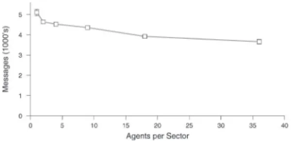
Our first evaluation metric is the total amount of com-munication that occurs in the system. Figure 2 shows that as the number of agents in each sector increases, and there are correspondingly fewer sectors overall, the amount of communication traffic decreases. Because each sector re-quires a certain amount of control messages, the total num-ber of messages is reduced as the numnum-ber of sectors de-creases. A more detailed view of the effects this change has on messaging will be shown later in Figure 4.

3.2. FUNCTIONAL DIFFERENTIATION

The varied assignment of roles forms a different, functional organization [5] in the system. Agents specialize their functionality in order to restrict the type of interac-tions which must take place between agents. For example, to obtain information about available sensors, a track man-ager must only contact the relevant sector manman-agers, in-stead of blindly broadcasting to all sensors [22]. Concen-trating the track management functionality into individual agents serves a similar role, by limiting the number of inter-actions necessary to resolve conflicts in sensor usage.

Although this type of functional decomposition does reduce the total number of interactions an agent might need to make, it can also increase that number for particular indi-viduals in the environment. For example, we have seen how the sector manager is responsible for disbursing informa-tion about the sensors in its sector, which facilitates the track manager’s discovery process. However, by serving in this capacity, it also makes itself a center of attention, which can result in unreasonable load when demand is high.

Consider Figure 3, which shows how much agents in the population differ from one another in their communi-cation habits, as the sector size changes. This notion is captured by measuring the standard deviation in communi-cation activity (total messages sent) exhibited by individual agents. If all agents are roughly the same they will have a low deviation, while a population that has a handful of out-lier agents with significantly higher message traffic will have a high deviation. As the number of agents in each sector increases, this graph shows an increase in disparity, be-cause a few agents are communicating more than their peers. Since the environment and target spacing are uniform, the differences can be attributed to the roles those agents take on. The rise in deviation when there is a single agent per sector represents the coexistence of the sector and track manager roles, because all agents act as sector managers when there is only one agent in each sector. This trend demonstrates that as the sector size grows, specialized agents such as sector and track managers can become “hotspots” of activity. In a bounded environment with un-reliable communication this concentration of activity could Recall that our initial intent behind creating these

sectors was to reduce the communication burden. The re-sults in Figure 2 are in some sense contradictory of this goal, because they show that the unpartitioned environ-ment had the lowest communication overhead. The parti-tioning process described in Section 2 results in the cre-ation of loose coalitions of sensors based on geographic location. Sector directory information, new target scan schedules, discovery measurements and certain tracking control messages are all contained within or directed to these coalitions. Because the manner in which this informa-tion being communicated is determined by the sectors, the sectors’ average size and shape has a tangible effect on some aspects of the system’s performance. If the sector is too large, and contains many sensors, then the communica-tion channel used by the sector manager may become satu-rated. If the sector is too small, then track managers may expend a great deal of time and bandwidth updating sector managers as its target moves through the environment. So, although these result show that large sectors have lower total overhead, the individual picture is not so straightfor-ward. This is covered in more detail below.

Although not shown in this figure, partitioning can also affect reactivity, because time may need to be expended to discover sector information. A track manager, for example, must perform queries to obtain sensor information as its target moves to new sectors. Smaller, more numerous sec-tors will result in delays caused by the additional queries, which ultimately affects the number of measurements it re-ceives. This delay will be revisited in Section 4.

Figure 2 - Affect of sector size on messaging

14

lead to reduced performance and data loss if the communi-cation channel becomes overloaded.

A growing tension between sector sizes is made apparent by these results: Figure 2 shows that smaller sec-tors lead to increased message traffic, and while Figure 3 shows that larger sectors imbalance load in the population. Although not shown, similar trends were observed in agents’ local workload levels, which track the number of non-com-municative actions being performed. Both characteristics are bad, so a compromise must be sought between them in the selected organizational design.

3.3. ORGANIZATIONAL MAINTENANCE

As insinuated above, there are costs associated with creating and maintaining the organizations employed by this design. The most frequently updated aspect of the organization is the relationship formed between track and sector managers, because the sectors interacted with by the track manager change as the target moves. This results in a class of control messages dependent on sector size. For example, as the target moves into part of the environ-ment the track manager is not familiar with, the manager must query the sector manager of that area to discover local sensors. Once those sensors are known, data collection commitments can be established.

As the target is tracked, the nearby sector managers must also be notified of the target’s estimated position.

Figure 4 provides a quantitative view of this over-head. As sector size increases, fewer directory and tracking control messages are necessary, because there are a fewer sectors to interact with as the target moves. In addition, the number of measurements increases as the sector size in-creases, because the reduced time spent by the track man-ager interacting with the additional sector manman-agers allows more time to be spent requesting data. More measurements results in a lower root-mean-squared (RMS) error between the measured and actual track, as seen in Figure 5.

The technique of migrating the tracking responsibil-ity through the agent population as the target moves is another example of how locality can be exploited. Signal attenuation conspires to make communication less reliable as distance increases. Multi-hop protocols can maintain reliability, but will increase end-to-end latency at each hop. Lacking the capacity for movement, the initial manager se-lected to track a target will therefore become less effective as the target moves away from it. By migrating this task to follow the target, the organization is able to retain locality despite the fact that the sensors themselves are immobile. This results in a reduction in the average distance that mes-sages must travel.

Figure 6 shows the effect track manager migration has on the average distance of communication. Because migration is triggered by sector boundaries, the tracking task will migrate less frequently when sectors are large, simply because they cover more area. Conversely, a lower average communication distance is observed when sectors are smaller. The lower migration rates also contribute to the increased measurement totals from Figure 4. Each migration interrupts the collection process as the role is moved from one agent to another, so the more frequently this transfer takes place, the more the average overall collection rate will be reduced.

Figure 4 - Message types vs. sector size

Figure 5 - Effects of sector size on RMS error

These metrics contribute to the organizational ten-sion. Large sectors improve the system’s RMS error rate, while smaller sectors exhibit better communication locality.

3.4. SCALABILITY RESULTS

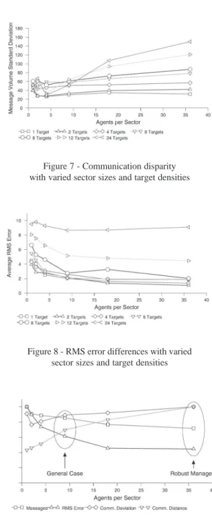
To explore the generality of these trends, we per-formed na additional set of experiments that varied num-bers of targets. Each test contained between 1 and 24 equally distributed targets, all of which moved concurrently through the environment for the duration of the experiment. The scenario was otherwise identical to those in Section 3. Fig-ure 7 shows that our original communication disparity pro-file from Figure 3 is maintained as the target density is var-ied, and the amount of disparity increases with the number of targets. Intuitively, this is because the amount of work particular agents are performing is tied to the number of targets in the environment. The communication load of the sector managers, for example, is directly proportional to the number of track managers it must interact with. This is par-ticularly true as the sector size increases – in the most ex-treme case a single sector manager must support all 24 track managers.

Similarly consistent results are seen for the systems RMS error, in Figure 8. The RMS error profile is maintained, although the baseline RMS error increases because the bounded sensing capabilities result in fewer average mea-surements per target. Notice how the RMS value for 6 and fewer targets are clustered together, while those with 8 or more become progressively worse. This is caused by a phase transition that occurs between 6 and 8 targets, when the number available sensors is no longer sufficient to meet demand. The inevitable reduction in the number of mea-surements track managers receive leads to an increase in RMS error.

Additional tests were performed which also varied the number of sensors in the environment, using six differ-ent configuration with between 9 and 81 sensors [7]. Re-sults from those experiments concur with the trends out-lined above.

The conclusion we draw from these experiments is that a tradeoff exists between communication volume and its distribution over the agent population. Message vol-ume decreases when there are more agents per sector be-cause fewer interactions are needed to obtain information, as shown in Figure 2. However, this shift can cause indi-vidual agents to incur a disproportionate communication burden, as shown in Figures 3 and 7. Figures 4, 5, and 6 show that organizational maintenance causes a similar tradeoff - larger sectors have lower overhead and better RMS error, while more track migration in smaller sectors increases communication reliability.

4. D

A

M

Our long-term objective is to use results such as these to make architectural design decisions. A simple strat-egy might compare the metrics graphically, and select a point which seems appropriate for the expected conditions. Normalizing and overlapping the trends from Section 3, pro-duces the graph in Figure 9. By searching for a common inflection point in this diagram, we can conclude that a sector size between 4 and 9 strikes an acceptable balance

Figure 7 - Communication disparity with varied sector sizes and target densities

Figure 8 - RMS error differences with varied sector sizes and target densities

16

between the competing positive and negative characteris-tics. This supports our hypothesis that a sector size be-tween 6 and 10 was a reasonable choice. However, the no-tion of “reasonable” is problemspecific, depending on the characteristics of the agents, the resources they use, and the environment. For instance, if more robust managers were available to handle the increased load, this graph also shows that better RMS performance can be obtained by using larger sector sizes. In general, the requirements imposed by goals and the capabilities of the system and environment guide an appropriate selection, and these experiments only suggest a course of action for a particular configuration.

The use of a more formal, analytic model that incor-porates the various characteristics can evaluate a wider range of candidate designs. Instead deducing metrics from a graph as above, one can create a function that takes re-quirements and characteristics as inputs, and produces a prediction or rating as output. To do this, one must capture the system’s behaviors in an abstract, quantitative model that provides a good approximation of the real system. We will do so by predicting role-specific values over the life-time t of the role. As before, we assume that the sensors and targets are uniformly distributed in the environment, and targets move with constant velocity. One could relax these assumptions by estimating interaction probabilities; al-though the calculations would be more complex, the spirit of the analysis would remain the same. Similarly, one could determine case peak performance by assuming worst-case densities. The formulas presented below do not repre-sent actual message totals, but are meant to reflect relative growth rates. As we will show in Figure 10, quantitative results can be obtained through the addition of appropriate constants. Consider the sensor manager. We will define the number of measurement messages sent by the sensor man-ager as its measurement load ( ). Measurements are taken in response to track manager requests, which are in turn prompted by targets in range of the sensor. is therefore dependent on the likelihood that a target is within its range

r. Assume T targets in an environment of area A, each with m measurements per time unit. can then be approxi-mated with the following equation:

So, as the number of targets increase, or the envi-ronments area decreases, the number of measurements will approach tm. This model is an upper bound, however, as it does not take into account track managers’ specific behav-iors, such as delays or inefficiencies that could affect the rate at which measurements are requested. These will be made more explicit in our model of the tracking process below.

The sector manager’s load ( ) is dependent on both the size of the sector and the number of targets. As we have observed earlier, larger sectors mean more sensors must be registered, as well as an increased probability that a target will be in the area. can be broken down into the one-time costs associated with sector creation, when the sensors send descriptions of themselves to their sector manager, and the continuing costs derived from targets moving though the sector:

N is the total number of sensors in the environment,

and u is the frequency at which target updates are supplied to the sector manager by the track manager. S is the actual size of the sector’s area, while is the effective size of the sector’s area. S and are differentiated by what they repre-sent. S is the strict bounding area of the sector we have been discussing thus far; membership in the sector is de-fined by containment within that area. is the potentially larger area over which measurements can be taken by sen-sors in that sector. If for example each sensor has a range of

r = 20, then will be the area bounded by S unioned with a

perimeter of width 20 surrounding S. Because it is this ef-fective area that determines when a track manager provides the sector manager with target location updates, grows in proportion with . The second term in the summation represents the directory queries it must respond to as tar-gets enter its sector, which depends on the velocity of the target v and the average distance the target must cross before it reaches a new sector. This latter term depends on the probability of target turns and the shape of the sector itself; we model it with a very coarse estimate of the average chord length in the sector .

Ignoring the effects of uncertain measurements or faulty data fusion, and assuming a reasonable choice of sensors are requested, the RMS error of the tracking pro-cess is primarily dependent on the number of measurements that are received over the lifetime of the track. In the absence of hindering factors, the track will receive mea-surements at a uniform rate m from each of c sensors used (we assume c is sufficient for triangulation purposes). The actual rate of measurements will be less than this, affected by the number of sensors that are used and any delays incurred by overhead tasks. In particular, the collection of sector directory information, and task migration when the target has grown too distant can reduce the total number of measurements that are obtained. Competition for sensors by other targets can also reduce the measurement rate.

(1)

Equation 3 defines , the number of sensors that will actually be used to track the target. It is bounded above by the desired quantity c, and below by the expected propor-tion of the total number of sensors that are in range of the target with radius b. This captures the effect that sensor density has on track quality. s models the proportion of a potentially contended sensor’s time usable by the target. If we assume the sensor is shared equally among targets, then the measurement rate obtained by an target will be inversely proportional to target density. As sensors come under contention, an allocation strategy must be employed to resolve the conflict [15]. An additional reducing factor models this optimization process; l estimates the amount of conflict, while λ controls how much the conflict degrades performance. When the target moves into a new area, there will be a delay d before the appropriate information is re-ceived. An additional delay g is incurred during track migra-tions when the target has moved two sectors away from that of the track manager. The net effect i of these delays and the corresponding increase in measurements when sec-tor sizes grow is supported by Figures 4 and 5.

To evaluate the accuracy of track measurement model, values were determined for each of the variables is dependent on. Most could be determined directly from the system’s configuration (e.g. the number of sensors N), through simple measurements (e.g. the directory service delay d), or by estimation (e.g. the average cross-sector distance ). The degradation constant λ required a more

detailed performance evaluation to find an appropriate value. In practice, if a complete prototype is not available to make a determination, one could approximate such values through targeted simulation of the appropriate subsystem [8], through formal analysis of the algorithm or technique in question, or by using a backof-the-envelope estimate that is revised as additional data is available. Figure 10 shows a comparison of the previously observed number of mea-surements and the predicted obtained from Equation 7 using these values.

Although the detailed results are not presented here, similar analytic models were also created for estimating the load placed on track managers [7].

5. U

O

M

The analytic models presented in the previous sec-tion, although individually precise, lack the cohesion nec-essary to create a complete prediction of system perfor-mance. There is no strong notion that particular and dis-tinct entities exist with associated characteristics. There is no well-defined way of specifying what decisions must be made, what values must be optimized over, or what con-straints must be respected. Instead, such individual expres-sions provide performance characteristics piecemeal, and comparative analysis of entire systems is performed later in an ad hoc manner. For example, note the discontinuity be-tween the measurement requests predicted by Equations 1 and 7. While we could copy the appropriate logic into Equa-tion 1, this duplicaEqua-tion of effort is somehow dissatisfying, and the resulting equations would still fail to capture the underlying relationship at the root of the problem. Finally, while the provided equations are able to model the effects of a changing sector size, we believe a single, static set of equations will be unable to represent all the alternative ways that a structure might be created in a concrete and accurate manner. For example, consider if there were a choice of the type of sensor or agent available for use in the environ-ment, or different tracking techniques that might be em-ployed, or an optional information aggregation hierarchy of arbitrary height and width. While one could create indi-vidual models for each dimension, combining them together in a coherent and expressive way would be challenging. It is for this reason that we view tools that operate principally on such representations, such as nonlinear solvers and queuing networks, as too limiting for our purposes (although we believe they may play a role in certain aspects of design evaluation).

To address this deficiency, we have developed a more robust set of tools to capture organizational informa-tion in a single, unified structure. The Organizainforma-tional De-sign Modeling Language (ODML) provides domain-inde-pendent mechanisms to model, evaluate and compare a

1 8

riety of organizational styles, including the sensor network we have described in this paper. As we will show, ODML incorporates quantitative information in the form of math-ematical expressions similar to those used above. These expressions are grouped into organizational constructs, connected via a graph of relationships, and ultimately used to represent and predict both the localized and global char-acteristics of an organization.

The immediate benefits of such a language are two-fold. First, by incorporating quantitative information about the environment, resources, agents, tasks, goals, or any other object relevant to the system’s performance, candi-date organizations may be tailored and evaluated in a con-text-specific way. For example, we may directly embed infor-mation about sensor density, target velocity, communica-tion limitacommunica-tions, and the like. This model can then be used to determine the organization which is most appropriate for that context, given a particular definition of utility. Second, once a suitable model hás been found, it can serve as an explicit organizational representation, guiding agents’ local decisions in a manner consistent with global objectives. The longer-term benefits of the organizational model in-clude being able to make predictions about runtime perfor-mance, which can be used to isolate and diagnose system failures and deficiencies. This same information can also be used to support adaptation of the system, by incorporating learned knowledge into the existing model and analyzing the resulting structure.

5.1. ODML

An organizational model, as we envision it, serves in several different capacities. At design time, it should be possible to use the structure to create and evaluate not just a single organizational instance, but an entire family of or-ganizational possibilities. At runtime, it should accurately describe the current organization. In both cases, the model must be sufficiently descriptive and quantitative that one can evaluate the organization’s effectiveness, and rank al-ternatives according to some specified criteria. Below, we enumerate the desired capabilities and characteristics a modeling language should possess to satisfy our require-ments:

1. Represent a particular organizational structure. This would include roles, interactions and associations (e.g., coalitions or teams). Different flows in the or-ganization, such as communication and resources, should be representable.

2. Represent the range of organizational possibilities, by identifying general classes of organizations and the parameters that influence their behavior. Differ-ent elemDiffer-ents should be modelable at differDiffer-ent levels of abstraction. Identify which characteristics are

under deliberate control, and which are derived from external factors.

3. Enable concrete performance predictions and allow deductive analysis by quantitatively describing the relevant characteristics exhibited by the structure, the manner in which those characteristics interact, and the constraints they are affected by. For example, both communication overhead and the effect that overhead has on work load should be represent-able.

Many different organizational representation schemes have been developed by researchers [1, 2, 3, 4, 9, 12, 16, 17, 18, 19, 24]. Most, if not all these representations can satisfy the first two points to varying degrees, but none are able to incorporate quantitative knowledge in such a way that concrete, organization-centric predictions can be made directly from the model itself. In this section we de-scribe a new formalism called ODML that explores how such information can be modeled and used.

Most existing representations fall into one of two categories: either they represent a wide range of organiza-tional characteristics abstractly, or they can capture a smaller set of characteristics concretely. The former are usually good at representing what entities or relationships exist or could exist, but cannot compare alternatives in a quantitative way. The latter may contain quantitative knowledge, but have difficulty relating that knowledge to specific organizational concepts, mitigating their usefulness if one is hoping to understand the effects a particular organizational design will have.

For example, OMNI [3] and [9] can each

capture a greater variety of organizational concepts than ODML, but do so in a largely qualitative way. Conversely, both SADDE [18] and MIT’s Process Handbook [16] can incorporate arbitrary quantitative information, but neither couples this information with the organizational structure in a way that enables one to deduce how the characteristics of one aspect of the design affect another. Decker’s TAEMS representation [1] does directly embed a certain amount of quantitative information, but this data is abstract and can only be used to make detailed performance predictions of a limited set of characteristics. The representation created by Sims [19] is perhaps closest in purpose to ODML. It incor-porates detailed quantitative information into a structured organizational model, but does not have the innate ability to evaluate and rank organizations based on this informa-tion. We also believe ODML’s more flexible design can model more situations at different levels of abstraction.

on which heuristics could be founded conspire to make the search for designs a potentially difficult task. In the end, each representation has its strengths, and ODML’s goal is not to supplant these works – but to demonstrate another approach that makes different tradeoffs. As shown below, ODML does so by incorporating a concrete but flexible set of primitives that can model a range of organizational con-structs along with the quantitative characteristics that dif-ferentiate them.

We continue by formally defining an ODML tem-plate specification as follows:

The foundation of the ODML template specification is the set of node templates, each of which corresponds to a particular physical or logical entity which might exist in the organization. For example, in our sensor network sce-nario there would be nodes corresponding to sectors, man-agers, relationships, agents and the environment, among other things. Each node N contains a number of elements, defined below:

t The node’s type. This label must be unique within

the set of template nodes that make up the organiza-tion.

The node’s instance limit. This specifies the

maxi-mum number of instances of the node type permit-ted in a valid organizational instance.

An ordered list of parameters that must be passed

to the node’s template when an instance of the node is created. These are analogous to the parameters one might pass to an object constructor. Each pa-rameter is specified with a type and local name.

I The set of node types that this node has an is-a

relation with using conventional object-oriented in-heritance semantics. If we assume that a node’s I =

{a, b}, an instance of the node will also be an

in-stance of a and b, possessing the characteristics of

all three node types. Isa relationships cannot be cyclic, i.e., N cannot have itself as a decedent.

H The set of node types that this node has a has-a

relation with. If we assume that H = {a, b}, an in-stance of the node will possess some number of instances of both a and b. It is through this type of relationship that the primary organizational decom-position is formed. Each hasa has a magnitude that specifies the number of instances connected by the relationship.

C A set of constants that represent quantified

charac-teristics associated with the node. Constants may be defined with numeric constants (e.g., 42), or math-ematical expressions (e.g., x + y).

K A set of constraints. Also defined with expressions,

na organization can be considered valid only if all of its constraints are satisfied.

M A set of modifiers that can affect (e.g.,

mathemati-cally change) a value contained by a node. Multiple modifiers may affect the same value. Modifiers model flows and interactions by allowing the characteris-tics and decisions made in one node to affect those of another.

V A set of variables, representing decisions that must

be made when the node is instantiated. Each vari-able is associated with a range of values it can take on. For example, a node might have a variable x that

2 0 symbol refers to a user-defined string, similar to a

variable name in a conventional programming language. These typically describe or refer to a particular characteris-tic. Type is the type name of some defined node, so

such that N.t = type. expression is an arbitrary algebraic expression, possibly referencing constants, symbols and function calls. ODML supports the use of floating point values, lists of floating point values, and discrete probabi-listic distributions in these expressions.

The top-level organization node also contains the elements H, C, K, M, V, providing a location to embed addi-tional global information and constraints.

Collectively, we refer to C, K, M, V as a node’s fields, and the quantitative state of a field as its value. For ex-ample, a constant field total load might be defined with the expression total_load = work_load + communication_load and have a value of 0.9 for a particular agent. Note that the use of the term “constant” may initially be misleading. While the expression defining total_load is fixed, the value for

total_load produced by that expression may change

through the application of modifiers, or due to changes in fields or values that the expression is dependent on.

At first glance, the ODML language may appear to be devoid of almost all the organizational concepts that are provided by typical organizational representations. This is partially true, and by design. Instead of directly incorporat-ing the usual high-level organizational components, such as hierarchies, roles, agents, etc., ODML provides a set of relatively low-level primitives by which such structures can be defined. For example, a node with the user-defined type

manager, having a has-a relationship with another node of

type agent could embody a role-agent relationship. A se-quence of has-a relationships between nodes could indi-cate a hierarchy.

Although the high-level semantics for these nodes may only be implicit, the concrete characteristics and de-sign ramifications are still directly and quantitatively cap-tured by the nodes’ fields. We feel that this approach can lead to an increased diversity of representable structures, by avoiding the assumptions and inevitable restrictions that typically accompany high-level structures.

ODML instances are quite similar to ODML tem-plates. The difference is that where a template is a descrip-tion of what could be, an instance is a descripdescrip-tion of what

is. Where a template might specify that a manager role can

be assigned to a single agent or distributed across multiple

agent nodes, na instance would indicate that manager_1 is

distributed across agent_5 and agent_7, and so on.

Instances are created by making choices for the de-cision points embodied in the template. Such dede-cision points are captured in two different ways: in the choice of value to assigned to a variable field, and in the choice of node type

to satisfy has-a relationships. Although employing just these two choice types may seem limiting, we have been able to use these simple concepts to capture many types of organi-zational possibilities. For example, a variable could be used to express the range of possible sensors_per_sector in the DSN domain, to controls the shape of part of the organiza-tion. Other uses of variables might be to decide the relative priority of an agent’s tasks, the amount of time it is willing to wait for a response, or the number of agents that will be used to form a coalition. Decisions made for the agent has-a relhas-ationships in the three roles will determine the specific role-agent bindings that will be used. Sequences of similar decisions could also decide if the manager role will be distrib-uted, or how tall a data processing hierarchy should be. Decid-ing upon the correct decisions can be viewed as a search process, which is a subject of ongoing work. Once an instance has been created from these decisions, the expressions de-fined by the fields, the data passed in through parameters, and the interactions caused by relationships can all be used to predict values for an individual node’s characteristics.

The formal definition of an instance is nearly identi-cal to that given in Equation 8, so we will not repeat it here. The differences principally relate to the replacement of node types in the template with instances of those nodes in the organizational instance. Thus, the set is the set of node instances, whose individual types no longer need be unique. So, where there might be just a single manager type in the template, there can be an arbitrary number of manager in-stances in the instance. Both is-a (N.I) and has-a (N.H) relationships no longer reference node types, but particular node instances in . Finally, the set is filled with appro-priate values from each node’s parent, and the variable set

V for each node is replaced by a single item from that

variable’s range. Because a common syntax is shared be-tween the two forms, for the remainder of this document I will indicate where necessary which is being considered.

As mentioned above, it is the ability to use an ODML model to deduce quantitative values for specific character-istics that sets it apart from other representations. The man-ner in which these values are determined for an instance node’s characteristics is defined by the pseudocode in Fig-ure 11. Note that some aspects of get value’s behavior, such as the manipulation of list-based data, have been omit-ted for clarity. This function shows how various sources of information, non-local data and node interrelationships all interact to describe the features of a particular node. It is through the execution of this function on a particular sym-bol that predictions are made of the design’s performance. For example, agent.get_value(total_load) would return a prediction of agent’s total_load.

Intuitively, an ODML instance is valid if all nodes’ constraints are satisfied, and the number of each type of node respects the limit (if any) specified by the template.

5.2. SENSOR NETWORK MODEL

The capabilities of ODML are best explained through na example.We will proceed with an overviewof how an ODML model was produced for the distributed sensor net-work domain described in Section 2. For clarity, we will rep-resent particular nodes, or fields that reside in the nodes, in italics. Space precludes showing the complete textual model

constructed for the sensor network, however, a portion of the model can be seen in Figure 12. The complete model is roughly 280 lines long, including whitespace and comments. A corresponding graph showing some aspects of the model’s template can be seen in Figure 13a. Vertices in that graph, such as sector and sensor, represent nodes. Nodes can represent both tangible (e.g. agent) and intangible (e.g.

sector) entities. Directed edges with a solid arrow represent

has-a relations, and the corresponding label indicates the magnitude of that relation. For example, each track_manager node has a number of agents defined by the field

num_agents. The corresponding definition is shown in line

4 of Figure 12.

A hollow-arrow edge represents an is-a relation, so

normal_agent is an instance of agent. Shaded nodes, such

as agent are abstract, and cannot be directly instantiated. Thus, any node with a has-a relation with agent can instead substitute normal_agent. This level of indirection allows this model to represent and easily use agents with different capabilities. For example, the robust_agent mentioned in Section 4 is represented with a node that also has an is-a relation with agent, and can be substituted for agent in the same way.

Figure 13b shows a particular instance of the tem-plate from Figures 12 and 13a. Vertices in the instance graph represent nodes, and a gray directed edge indicates the existence of a non-local modifier from the source node to a field in the target node. Black directed edges represent has-a relhas-ationships, but unlike the templhas-ate they hhas-ave no lhas-abels. Because this is a particular instance of the sensor network organization, the decision points present in the template have all been decided. Therefore, where sector might have the num_sensors label on its sensor relationship in the tem-plate, a discrete value of two has been chosen for that field in this particular instance. Because of this, each sector in the instance has two sensors (S). Normal agents (a), sector managers (SM), track managers (TM), and two kinds of track manager relations (SM-TM and S-TM), are also present.

We can relate this model directly to the organiza-tional structures discussed in Sections 3.1 and 3.2. Geo-graphic coalitions are embodied in the sector node. The size of the has-a relation sector has with the sensor node reflects the chosen sector size, and the sector manager is specified with the sector_manager node. The functional differentiation aspect is modeled directly by the

sector_manager, track_manager and sensor nodes. Each

represents a role that can be assigned. This assignment is represented with the agent has-a relationship each node possesses. The particular instance of agent node associ-ated with a role node corresponds to the particular agent assigned to that role.

Figure 11 - Pseudocode for the get_value function of a node N . This function is used to quantify

2 2

The heart of any ODML model exists in the expres-sions encoded within nodes’ fields. A selection of these fields, contained by the track_manager and s tm_relation nodes, are shown in Figure 12. The former defines the track manager role, while the latter represents the relationship that role hás with sensors in the environment. Each node’s field may contain an arbitrary mathematical equation, com-bining local and nonlocal information to calculate new local values as depicted in Figure 11. These expressions provide a way for the designer to represent how different character-istics of the node may be computed. For example, suppose

we wish to define how to calculate the track manager’s logi-cal footprint (area) of a target as it moves through the envi-ronment. This área will depend on the amount of uncer-tainty the manager hás in the target’s location, along with a factor modeling the target’s “area of influence”, that relates to the effective sector size discussed in Section 4. In our model, this area will be a circle; line 11 shows how the

target_area of a track manager is derived from the target’s influence_radius. The number of sensors presumed capable

of sensing the target is the average number of sensor which lie within the target area. Therefore, although the number of

Figure 12 - A portion of the raw ODML specification for the track_manager and s_tm_relation nodes

desired_sensors is independent of the environment, the actual_sensors_available to the manager will depend

indi-rectly on the target_area and sensor_density, as shown in line 16. The requested_sensors will be the minimum of the desired and available.

We may model the number of measurements pro-vided to the track manager in a similar way. The actual

measurement rate in the sensor-track manager relationship

is derived from the locally calculated requested

measure-ment rate and actual measuremeasure-ment ratio computed by the

sensor node. This value is then used in a pair of modifiers defined in lines 31 and 32 that specify for the track manager and sensor the actual number of measurements that will be taken.

In this way, the characteristics of one node may af-fect or be afaf-fected by those of another. Oscillations and infinite recursion are avoided by allowing only acyclic equa-tion relaequa-tions. The resulting web of equaequa-tions allows one to model important concepts such as information flow, control flow, and the effects of interactions. By propagating data through these expressions, the model can predict the char-acteristics of both individual nodes and the organization as a whole. Perhaps more importantly, it also allows the model to predict characteristics not necessarily envisioned or con-sidered by the designer, as the results of expressions can flow through the graph in unanticipated ways. It is this automatic propagation which differentiates an ODML model from a simple set of equations, by creating a unified view of the complete working organization.

The mechanisms provided by the ODML primitives allows one to model a range of common, organizationallyinfluenced system characteristics. To con-tinue our example, we will describe several such character-istics relevant to the sensor network organization, and dem-onstrate how the interplay between such elements results in a more coherent, unified model.

5.2.1. Environmental and System Constants

Incor-porating numeric constants within an ODML structure, a crucial element of any realistic model, can be at once simple to accomplish and difficult to complete successfully. The definition itself, comprised of a straightforward constant field, is trivial to create. Determining what value to place within this field can be an entirely different matter, just as with the values used in the discrete analytic models. For example, the desired_sensors constant at Figure 12 line 14 is a known quantity that can be extracted directly from agent code or a software engineering specification. On the other hand, the uncertainty_radius on line 9, which represents the expected radius of the target’s uncertainty bound, can be more difficult to determine directly. Assuming for the moment that this value does not depend on other

charac-teristics (such as the target’s velocity), one could first specify a rough estimate, and later revise that estimate if contradictory empirical evidence is observed in practice or a more accurate value is devised. In practice, most of the numeric constants in the sensor network model were de-rived through a combination of known system parameters, estimation based on domain expert knowledge, and in some cases, instrumentation of a running system or prototype.

The specification of expression-based constants can be accomplished in a similar fashion, although these are more frequently determined based on knowledge of the system in question. An example of this is the track manager’s

requested_sensors in line 17 of Figure 12. This represents

the number of sensors that manager will actually ask for, which may be less than desired_sensors in the case where there is insufficient sensor density in the environment. It is sometimes the case, however, that a simple closed-form solution is either difficult to derive or not possible. In the former case, we have used curve-fitting techniques to ob-tain approximate expressions from empirical data. This techniquewas used to find a predictive expression for RMS error, based on the number of received measurements. It is worth noting that this particular expression attempts to ab-stractly and indirectly capture a number of complex effects, including the effects of target ambiguity, incorrect data fu-sion and the average quality of the measurements them-selves.

For the latter case, when a closed-form solution does not exist or cannot be found, ODML supports a general “mapping” function, which allows one to define a function correlating a discrete input value with an arbitrary expres-sion. With this, one may define some f such that, for

ex-ample, , etc. The average

effective_area of the sector nodes uses such a function.

This characteristic, originally defined as in Equation 2, represents the average area covered by the sensors in each sector, which is typically larger than the area of the sector itself. A mapping function was used to effectively create a look-up table, which associates an appropriate expression calculating the effective área for each sector size.

5.2.2. Agent Interactions The manner in which

2 4

modifier to add a corresponding number of messages to its

sector manager. We have used both modifiers and

param-eters to disseminate such agent characteristics so that they may be incorporated in remote nodes.

The second technique employs a more explicit rep-resentation, by creating an independent node to model the interaction itself. An example is s_tm_relation, the sensor-to-track manager relation, shown in Figures 12 and 13. This node models the interactions that take place between a track manager and a sensor, which include determining the rate at which task requests are generated by the track manager, the rate at which measurements are taken in response to those requests, and the rate at which corresponding results are sent back to the track manager. Each of these values is calculated using a combination of information from each entity, and the results applied back to the appropriate node. For example, the actual_measurement_rate is used to in-crement the sensor’s messages_rr constant, which tracks the number of result messages that are sent.

Choosing how to model an interaction depends on a number of factors. Simple interactions are typically embed-ded, thus avoiding the additional overhead associated with node creation.We have found that there are several ways that more complex interactions benefit from an explicit, sepa-rate model. By separating and encapsulating the interac-tion, its effects can be made more transparent and the model more understandable. In the case where there is a one-to-many type of relation, as with a track manager and the sen-sors it uses, this type of separation also facilitates the ex-pression writing process by limiting the scope that indi-vidual equations must cover. Finally, in the case where sev-eral alternative interaction styles are available, the explicit representation allows the designer to use variables or in-heritance to model and reason about such choices. For ex-ample, if our track managers had two different ways of re-questing measurements from a sensor, those alternative in-teractions could be modeled as s_tm_relation1 and s_tm_

relation2, each defined as an instance of s_tm_relation

with an is-a relationship. When an instance of

track_manager is created, one of those two alternatives

would be selected for each sensor, and the corresponding effects incorporated appropriately. In this way, in addition to representing the quantitative effects of interactions, the selection of agent interaction or coordination mechanisms may be cast as an organizational decision in ODML.

5.2.3. Multiple Role Assignments In human

organi-zations, individuals frequently act in many different capaci-ties, serving different needs and exhibiting different behav-iors depending on the working context. In some complex multi-agent systems, similar phenomena may be observed, where individual agents take on multiple roles that dictate the various responsibilities, capabilities and activities it is

associated with. Because the assignment of these roles to individual agents is na organizational decision, it is impor-tant represent both the assignment itself and the cumula-tive effects of that decision.

As mentioned earlier, there are three roles in our dis-tributed sensor network organization: the sector manager, the track manager and the sensor. These are represented by the sector_manager, track_manager, and sensor nodes, respectively. Role assignment is modeled through the use of a hasa relationship. Specifically, each of these role nodes has na agent, as shown in Figure 13a, that represents the particular agent that role is assigned to. During instantiation, has-a relations may be fulfilled in two different ways. Either a new instance of the target node is created to satisfy the relationship, or an existing instance of the node is used in the same way. Na example of the latter can be seen in Figure 13b, where the leftmost node a is owned by both SM and

S, indicating that particular agent has been assigned to two

roles.

Most of the detailed characteristics in this model are computed within the role nodes. Therefore, important as-pects such as load and resource usage are inherently sepa-rate and rolespecific. To capture the effects of multiple role assignments, these individual characteristics are first propa-gated into their relevant agent using modifiers. Each agent can then predict the cumulative effects of its roles. A natu-ral example of this in this is the propagation of communica-tion effects, which we have mencommunica-tioned earlier. In this case the communication load of the agent is computed to be the sum of the communication loads of the roles it takes on. If we wish to capture more complex situations, such as super-or sub-additive effects, the the agent load can be defined as some function of the various role loads that correctly ac-counts for those effects. This combined load can then be accessed and utilized by the individual roles in whatever manner in appropriate.

5.2.4. Dynamic Role Assignment In reactive or

adap-tive systems, roles are frequently created dynamically in response to emerging phenomena. Such is the case with the track manager role, which is assigned only when a new target has been detected in the environment. Although we can and do model rates of change and expected value, there is no explicit representation of a varying timeline or change points in the model. Therefore, ODML instances generally represent a snapshot of a running system, or an averaging of effects as they would occur over some span of time. If dynamic elements exist in the source environment or sys-tem, they may be represented in that same manner. For ex-ample, although at any given point in time there may be many or few targets in the environment, there is some ex-pected number of targets that represents a statistically av-erage value. This number would then be used to estimate the “normal” situation, and be reflected in the model ac-cordingly. ODML also natively supports the use of discrete probabilistic distributions, allowing one to explicitly repre-sent a finite set of possible conditions. Furthermore, be-cause ODML is based on sets of arbitrary equations, one could also use continuous distributions (e.g., Poisson), pro-vided the means to analyze them can be expressed using closed-form expressions. For example, by encoding the ap-propriate parameters as constants (e.g., x,λ) and then ma-nipulating those values using traditional queuing theory techniques [10], one can integrate and estimate behaviors based on these more complex assumptions.

Additional dynamism is present in the sensor net-work example, due to the migration of the track manager role as described in Section 2. When this role moves to maintain locality with its target, the effects of that role are effectively spread over multiple different agents. To represent this ef-fect, the model uses the target’s velocity and the sectors’ sizes to first estimate how frequently that role will migrate. Because this is a rate, it must be combined with the duration of the scenario to determine the number of agents that role will be assigned to. This number is then used to calculate

num_agents, which as mentioned earlier is used to specify

the size of the track manager’s agent has-a relationship. So, if the model predicts that the track manager role will be created and then migrate twice, the num_agents field in

track_manager will be set to three. The role’s relevant

char-acteristics are divided and distributed evenly among those three agents using modifiers as described previously.

5.2.5. Heterogeneity Another important advantage

that ODML offers over the simple analytic models from Section 4 is that heterogeneity is more readily represent-able. When calculating the total number of measurements for a track in Equation 7, for example, we assumed that all sensors would produce measurements at equal rates. Simi-larly, the sector manager’s load in Equation 2 assumed that

all targets moved with equal velocity. Neither of these sim-plifying assumptions are likely to be true in practice, so to the degree the unified model can represent such additional information, it will have a decisive advantage in accuracy.

ODML’s ability to model heterogeneity is derived from the the node-based representation of entities. Because each role, agent or other structure is defined as a separate node in the organizational instance, entities that share a common type may still contain different values or be af-fected by different organizational pressures and flows.We have seen examples of this in the previous two sections. Because agents may be assigned single or multiple roles, the resulting agent population has the potential to be het-erogeneous in the final organization. These variations may then propagate through the organizational instance to cre-ate differences elsewhere in the model. For example, com-munication load can be tied to the agent’s capacity to per-form work, which could affect the number of measurements its sensor role could take, which would affect the RMS error of the track manager using that sensor.

Inheritance provides an additional mechanism to represent heterogeneity. For example, to model the “robust managers” scenario from Section 4, we defined a robust_

agent node that has an is-a relationship with agent. This

effectively creates two different classes of agents that can be employed, each with potentially different capabilities and costs.

5.2.6. Conflicts, Constraints and Resolution Many

of the more interesting aspects of organizational models revolve around the limits or constraints that are imposed on the system, and what happens when those limits are ap-proached or exceeded. ODML models can represent both hard and soft constraints. The former include conditions which the designer has deemed untenable, while the latter are usually characteristics that degrade more gradually, and may be tolerated by the system.