Braz. J. Phys. vol.35 número1

The Interacting Gluon Model: a review

F.O. Dur˜aes

, F.S. Navarra

, and G. Wilk

1

Dep. de F´ısica, Faculdade de Ciˆencias Biol´ogicas, Exatas e Experimentais, Universidade Presbiteriana Mackenzie, C.P. 01302-907 S ˜ao Paulo, Brazil

2

Instituto de F´ısica, Universidade de S˜ao Paulo, C.P. 66318, 05389-970 S˜ao Paulo, SP, Brazil

3

A. Soltan Institute for Nuclear Studies, Nuclear Theory Department, 00-681 Warsaw, Poland

Received on 15 December, 2004

The Interacting Gluon Model (IGM) is a tool designed to study energy flow, especially stopping and leading particle spectra, in high energy hadronic collisions. In this model, valence quarks fly through and the gluon clouds of the hadrons interact strongly both in the soft and in the semihard regime. Developing this picture we arrive at a simple description of energy loss, given in terms of few parameters, which accounts for a wide variety of experimental data. This text is a survey of our main results and predictions.

1

Introduction

1.1

Why a model?

After more than 30 years of continuous advances we might expect that Quantum Chromodynamics (QCD), the estab-lished theory of strong interactions, would provide us with a satisfactory understanding of high energy hadronic reac-tions. Unfortunately this is not yet the case and we have to study these reactions using models instead of the theory. This is so essentially because of two reasons. The first one is because we can only perform reliable calculations in the perturbative regime, i.e., in reactions where the momentum tranfer is larger than a few GeV. However these represent only a small fraction of the hadronic cross sections. In-deed, even at very large energies most of events involve low momentum transfer, as indicated by the average transverse momentum of the produced particles, which is, in most of the experiments, of the order of 1 GeV or less. The sec-ond reason is that the number of interacting particles may be so large that many body techniques and approximations are needed. At RHIC, for example, the number of finally pro-duced hadrons may be as large as 6000 (!) resulting from the complicated interaction among a similar number of quarks and gluons at the initial stage of the collisions. The study of these systems can not be made from first principles and models are required.

1.2

What is a good model?

Since making models is inevitable and since there has been a proliferation of models for particle production, we must try to establish criteria to decide when a model is better

than other. A condition to be satisfied by a model is a clear connection to the underlying theory, i.e., the use of the ap-propriate degrees of freedom with the correct QCD interac-tions. Moreover, assumptions should be made only where the theory is not applicable and the introduction of para-meters should be restricted to a minimum. Furthermore, a model must have predictive power and be testable. Even with these constraints there are many implementations of the basic QCD concepts and many different ways to treat the non-perturbative dynamics.

and extract the effective temperature. Here we have little input and little output but we may learn something study-ing different systems and, for example, establish the behav-ior of the temperature as a function of the collision energy. The model discussed here belongs to this cathegory of ”eco-nomic” models. Our aim is to decribe energy flow (stopping, energy deposition and leading particle spectra) with a sim-ple picture based on QCD, with few parameters and learn something from the analysis of data.

1.3

Why study energy flow?

Multiparticle production processes are the most complicated phenomena as far as the number of finally involved degrees of freedom is concerned. They also comprise the bulk of all inelastic collisions and therefore are very important - if not per sethen as a possible background to some other, more specialized reactions measured at high energy collisions. The large number of degrees of freedom calls inevitably for some kind of statistical or hydrodynamical descrition when addressing such processes. All corresponding models have to be supplemented with information about the fraction of the initial energy deposited in the initial object (”fireball”) which is then the subject of further investigations. This frac-tion is called inelasticity and it is relevant also for low energy nuclear reactions [7].

The knowledge of the energy deposited in the central rapidity region in heavy ion collisions at RHIC and LHC is crucial [8]. Dividing this number by the volume of the formed system, we will have an estimate of the initial en-ergy density in such collisions. If it is high enough we may be in a new phase of hadronic matter: the plasma of quarks and gluons (QGP).

On the other hand, the knowledge of the momentum spectrum of the particles measured in the large rapidity re-gion, and, in particular, those with the quantum numbers of the projectile (the so called leading particles or LP) gives valuable information about the non-perturbative dynamics of QCD. Moreover, the LP spectrum and the inelasticity of the reaction are very useful in cosmic ray physics, in the description of the evolution of hadronic showers in the at-mosphere [9].

In the model considered here we hope to extract infor-mation about the gluonic structure of hadrons from observ-ables like mass, diffractive mass and leading particle spectra, which are, at least in principle, very easy to measure. This model describes only certain aspects of hadronic collisions, related to energy flow and energy deposition in the central rapidity region. It should not be regarded as an alternative to a field-theoretical approach to amplitudes, but rather as an extension of the naive parton model. The reason for using it is that it may be good enough to account for energy flow in an economic way. The deeper or more subtle aspects of the underlying field theory probably (this is our belief) do not manifest themselves in energy flow, but rather in other quantities like the total cross section. Inspite of its simplic-ity, this model can teach us a few things and predict another few. This is encouraging because in the near future new data from FERMILAB, RHIC and LHC will be available.

1.4

A brief history of the IGM

Long time ago, based on qualitative ideas advanced by Pokorski and Van Hove [10], we started to develop a model to study energy deposition, connecting it with the apparent dominance of multiparticle production processes by the glu-onic content of the impinging hadrons, hence its name: In-teracting Gluon Model(IGM) [11]. Its original application to the description of inelasticity [12] and multiparticle pro-duction processes in hydrodynamical treatments [13] was followed by more refined applications to leading charm pro-duction [14] and to single diffraction dissociation, both in hadronic reactions [15] and in reactions originated by pho-tons [16]. These works allowed for providing the systematic description of the leading particle spectra [17] and clearly demonstrated that they are very sensitive to the amount of gluonic component in the diffracted hadron as observed in [18] and [19]. We have found it remarkable that all the re-sults above were obtained using the same set of basic pa-rameters with differences arising essentially only because of the different kinematical limits present in each particular application. All this points towards a kind ofuniversalityof energy flow patterns in all the above mentioned reactions. The IGM was further developed and fluctuations in impact parameter were included in [20], where a careful study of the inelasticity in proton-nucleus reactions was performed. The model was employed by the Campinas group of cosmic ray physics to reanalyse data from the AKENO collaboration and extract the proton-proton and proton-air cross sections [21]. This group used the IGM also to study the nucleonic and hadronic fluxes in the atmosphere [22].

In the next section we shall provide a brief description of the IGM, stressing the universality of energy flow and then we devote the other sections to discuss the applications of the model.

2

The model

The IGM is based on the idea that since about half of a hadron momentum is carried by gluons and since gluons interact more strongly than quarks, during a high energy hadron-hadron collision there is a separation of constituents. Valence quarks tend to be fast forming leading particles whereas gluons tend to be stopped in the central rapidity re-gion. The collision between the two gluonic clouds is treated as an incoherent sum of multiple gluon-gluon collisions, the valence quarks playing a secondary role in particle produc-tion. While this idea is well accepted for large momentum transfer between the colliding partons, being on the basis of some models of minijet and jet production [1,28-34], in the IGM (and also in [29] and [34]) its validity is extended down to low momentum transfers, only slightly larger than ΛQCD. At first sight this is not justified because at lower scales there are no independent gluons, but rather a highly correlated configuration of color fields. There are, however, some indications coming from lattice QCD calculations, that these soft gluon modes are not so strongly correlated. One of them is the result obtained in [35], namely that the typical correlation length of the soft gluon fields is close to0.3fm. Since this length is still much smaller than the typical hadron size, the gluon fields can, in a first approximation, be treated as uncorrelated. Another independent result concerns the determination of the typical instanton size in the QCD vac-uum, which turns out to be of the order of0.3fm [36]. As it is well known (and has been recently applied to high energy nucleon-nucleon and nucleus-nucleus collisions) instantons are very important as mediators of soft gluon interactions [37]. The small size of the active instantons lead to short dis-tance interactions between soft gluons, which can be treated as independent.

These two results taken together give support to the idea thata collision between two gluon clouds may be viewed as a sum of independent binary gluon-gluon collisions, which is the basic assumption of our model. Developing the pic-ture above with standard techniques and enforcing energy-momentum conservation, the IGM becomes the ideal tool to study energy flow in high energy hadronic collisions. Con-fronting this simple model with several and different data sets we obtained a surprisingly good agreement with exper-iment.

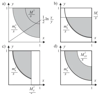
Figure 1. Schematic IGM pictures for(a)non-diffractive (ND),(b)

and(c)single diffractive (SD) and(d)double Pomeron exchange (DPE) processes.

Figure 2. Phase space limits of ND, SD and DPE processes in the IGM. The1

2ln

x

yline in a) indicates the rapidityY of the produced

massM.

The hadron-hadron interaction follows the simple pic-ture shown in Fig. 1: the valence quarks fly through essen-tially undisturbed whereas the gluonic clouds of both pro-jectiles interact strongly with each other forming a central fireball (CF) of massM. The two incoming projectilesp1 andp2loose fractionsxandyof their original momenta and get excited forming what we call leading jets (LJ’s) carrying xL= 1−xandyL= 1−yfractions of the initial momenta. Depending on the type of the process under consideration one encounters the different situations depicted in Fig. 1.

(SD) events (Figs.1b and c) the corresponding diffractive systems have massesMXorMY (comprising also the mass of CF). In double Pomeron exchanges (DPE) (Fig. 1d) a CF of mass MXY is formed. In Fig. 2 we show their corre-sponding phase space limits. The only difference between ND and SD or DPE processes is that in the latter cases the energy deposition is done by a restricted subset of gluons which in our language is a “kinematical” Pomeron (IP), the name which we shall use in what follows.

The central quantity in the IGM is χ(x, y), the prob-ability to form a CF carrying momentum fractions x and y of two colliding hadrons. It follows from the quantita-tive implementation of the ideas described above. The es-sential ingredients are the assumption of multiple indepen-dent gluon-gluon collisions, low momentum dominance of the gluon distributions and energy-momentum conservation. The derivation of our main formula, presented below, can be found in Appendix A.χ(x, y)is given by:

χ(x, y) = χ0 2π

Dxy

exp{− 1

2Dxy

[y2(x− x)2

+ x2(y− y)2+ 2xy(x− x)(y− y)]}

(1) whereDxy=x2y2 − xy2and

xnym=

xmax

0

dx′x′n

ymax

0

dy′y′mω(x′, y′), (2) withχ0defined by the normalization condition

1

0 dx

1

0

dy χ(x, y)θ(xy−Kmin2 ) = 1, (3)

whereKmin= m√_s0is the minimal inelasticity defined by the massm0of the lightest possible CF. The functionω(x′, y′), sometimes called the spectral function, represents the aver-age number of gluon-gluon collisions as a function ofx′ _e

y′_:

ω(x′, y′) = dn

dx′_dy′. (4) The appearance of the numberncomes from the use of Pois-sonian distributions, which, in turn, is a consequence of the assumption of independent gluon-gluon collisions.ω(x′_{, y}′₎ contains all the dynamical inputs of the model both in the perturbative (semihard) and non-perturbative (soft) regimes. The soft and semihard components are given by:

ω(S)(x′, y′) = σˆ (S) gg (x′y′s)

σ(s) G(x ′_)G(y′₎

× θ(x′y′−Kmin2 )θ( 4pT2min

s −x

′_y′₎₍₅₎ and

ω(H)(x′, y′) = σˆ (H) gg (x′y′s)

σ(s) G(x ′_)G(y′₎

× θ(x′_y′₋4pT2min

s ) (6)

whereσˆS

ggandσˆggH are the soft and semihard gluonic cross sections, pTmin is the minimum transverse momentum for

minijet production andσdenotes the impinging projectiles cross section.

The values ofxmaxandymaxdepend on the type of the process under consideration. For non-diffractive processes all phase space contained in the shaded area is allowed and in this case we have:

xmax=ymax= 1 (7)

The effective number of gluons from the corresponding projectiles are denoted byG’s and have been approximated in all our works by the respective gluon distribution func-tions. There has been a remarkable progress in the knowl-edge of the parton distributions in hadrons [38, 39, 40], es-pecially in the lowxregion, which becomes crucial at en-ergies in the TeV range. Since in our previous applications of the IGM we have been studying collisions in the GeV domain, there was no need to use very sophisticated parton distributions. Moreover, very often we needed parton den-sities at very low scales, which were not considered in the analyses presented in [38, 39, 40]. In some cases, we have used the parametrization of [41], which is better suited for small scales. However, as it will be shown, the IGM can de-scribe both the hadronic and nuclear collision data with the following simple form of the gluon distribution function in the nucleon:

G(x) =p(m+ 1)(1−x) m

x (8)

withm= 5and the fraction of the energy-momentum allo-cated to gluons is equal top= 0.5.

the amount of energy-momentump=pIP allocated to the impinging hadron and which will find its way in the object that we call IP. It turns out that pIP ≃ 0.05, whereas p ≃ 0.5 for all gluons encountered so far. This choice, with m = 5 in eq. (8), corresponds to an intermediate between “soft” and “hard” Pomeron (see Appendix B) and will be used in what follows. Just in order to make use of the present knowledge about the Pomeron, we have chosen σ(s) = σpIP = a+bln(s/s0)wheres0 = 1GeV2and a= 2.6mbandb= 0.01mb.

In single diffractive processes only a limited part of the phase space supporting the χ(x, y)distribution is allowed and in this case the integration limits in the moments of the spectral functionω(eq. (2)) depend on the massMXorMY that is produced:

xmax= 1 ; ymax=y ; xmaxymax=MX2/s (9) xmax=x ; ymax= 1 ; xmaxymax=MY2/s (10) By reducing these maximal values we select events in which the energy released by the projectile emitting IP is small and at the same time allow the formation of a rapidity gap betwen the diffractive mass and the diffracted projectile. This is the experimental requirement defining a SD event.

Double Pomeron Exchange processes, inspite of their small cross sections, are inclusive measurements and do not involve particle identification, dealing only with energy flow. Such a process was recently measured by UA8 [24] and used to deduce theIP IP cross section,σIP IP. It turned out that using this method one getsσIP IP which apparently depends on the produced mass MXY. This fact was ten-tatively interpreted as signal of glueball formation [24]. In the IGM a double Pomeron exchange event (Fig. 1d) is seen as a specific type of energy flow. The difference between it and the “normal” energy flow as represented by Fig. 1a is that now the gluons involved in this process must be con-fined to the object we called IP above. We are implicitly assuming that all gluons fromp1andp2participating in the collision (i.e., those emitted from the upper and lower ver-tex in Fig. 1d) have to form a color singlet. In this case two large rapidity gaps will form separating the diffracted hadron p1, the MXY system and the diffracted hadronp2, which is the experimental requirement defining a DPE event. Also in this case only a limited part of the phase space sup-porting theχ(x, y)distribution is allowed and the limits in the moments of the spectral functionω(eq. (2)) depend on the massMXY in the following way:

xmax=x ; ymax=y ; xmaxymax=MXY2 /s . (11) As beforeGIP(x)represent the number of gluons par-ticipating in the process and the cross sectionσ, appearing in eqs. (5) and (6), represents now the Pomeron-Pomeron cross section,σIP IP.

The clear separation between valence quarks and bosonic degrees of freedom does not appear exclusively in the IGM. It appears also in soliton models of the nucleon [42]. In the Chiral Quark Soliton Model [43], for example, the nucleon is made of three massive quarks bound by the self-consistent pion field (the ”soliton”). It is interesting to

observe that, according to this model, in a collision of two nucleons the valence quarks would interact much less than the pions and therefore would filter through and populate the large rapidity regions leaving behind a blob of pionic matter in the central region.

3

Inelasticity

The energy dependence of inelasticity is an important prob-lem which is still subject of debate [44]. Generally speak-ing, inelasticityKis the fraction of the total energy carried by the produced particles in a given collision. However in the literature one finds several possible ways to define it. In the first one, inelasticity is defined as

K1 = √M

s (12)

where√sis the total reaction energy in its center of mass frame andM is the mass of the system (fireball, string, etc.) which decays into the final produced particles. The second definition ofKconsidered here is

K2 = √1 s

i

dy µi dni

dy coshy (13)

whereµi =

p2

T i+m

2

i is the transverse mass of the pro-duced particles of typeianddni/dytheir measured rapidity distribution. These two definitions are, in principle, model independent, although the massMmight be difficult to eval-uate in certain models.

The main difference betweenK1andK2is that, whereas the first one refers to partons, the second one refers to final observed hadrons. K2 implicitly includes the kinetic en-ergy of the object of massM. From the theoretical point of view,K1is a very interesting quantity because it can be easy to calculate and because it is the relevant quantity when studying the formation of dense systems (e.g. quark-gluon plasma).

In Ref. [12] we used the IGM to study the energy de-pendence ofK1. We concluded that the introduction of a semihard component (minijets) in that model produces in-creasing inelasticities at the partonic level. In Ref. [13] we introduced a hadronization mechanism in the IGM, cal-culated the rapidity distributions of the produced particles, compared our results with the UA5 and UA7 data and fi-nally calculatedK2. The purpose of this exercise was to verify whether the hadronization process changed our pre-vious conclusion.We found that, whereas some quantitative aspects, like the existence or not of Feynman Scaling in the fragmentation region and the numerical values ofK2, de-pend very strongly on details of the fragmentation process, the statement that minijets lead to increasing inelasticities remains valid.

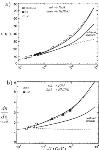
(Fig. 4a) and central rapidity density (Fig. 4b) together with the results of HIJING [1] for the same quantities.

Figure 3. Pseudorapidity distributions measured at the central ra-pidity region. Data are from the UA5 collaboration [45] at different energies and from CDF collaboration [46] at√s= 1800GeV. Full lines show the IGM results.

Figure 4. a) Average charged multiplicities as a function of the re-action energy. Squares and circles are experimental data. Full lines show the IGM results with and without the semihard contribution (lower curve). Dashed lines show the same quantities calculated with HIJING [1]. b) The same as a) for the central pseudorapidity distributiondn/dη|η=0.

Both models fit the data but differ significantly when one switches off the semihard (minijet) contribution. Whereas in HIJING Feynman Scaling violation in the central region (the growth of dn/dη|η=0 with

√

s) is entirely due to the minijets, in the IGM this behavior is partly due to soft in-teractions, there being only a quantitative difference when minijets are included.

In Fig. 5 we plotK2 (full lines) andK1 (dashed lines as a function of √s. The lower curves show the results when minijets are switched off and only soft interactions take place. The upper curves show the effect of including minijets.

Figure 5. InelasticitiesK1(dashed lines) andK2(solid lines) with

minijets (upper curves) and without minijets (lower curves) as a function of the reaction energy.

4

Leading charm and beauty

In Ref. [14] we treated leading charm production in connec-tion with energy deposiconnec-tion in the central rapidity region giv-ing special attention to the correlation between production in central and fragmentation regions. The significant differ-ence between thexF dependence of leading and nonleading charmed mesons [47] was not possible to be explained with the usual perturbative QCD [48] or with the string fragmen-tation model contained in PYTHIA [49].

In the case of pion-nucleon scattering, the measured leading charmed mesons [47] are D− _{and the nonleading}

areD+_{. In the spirit of IGM, the central production ignores} the valence quarks of target and projectile which, in the first approximation, just “fly through”. Because of this, the cen-trally producedD’s do not show any leading particle effect. There are, however, two distinct ways to produceDmesons out of LJ’s: fragmentation and recombination. We assumed that, whenever energy allows, we would have alsocc¯ pairs in the LJ (produced, for example, from the remnant gluons present there). These charmed quarks might undergo frag-mentation intoDmesons and also recombine with the va-lence quarks. WhereasD+_andD−_{mesons are equally}

pro-duced via fragmentation only “leading”D−_{’s (which carry}

the valence quarks of target and projectile) can be produced by recombination. It turns out that only this last process will produce asymmetry.

pairs can be attributed to the existence of a meson cloud around the nucleons and pions [50].

The asymmetry inD meson production can be defined as:

A(xF) = dσD−

(xF)

dxF −

dσD+ (xF)

dxF

dσD−_(x

F)

dxF +

dσD+ (xF)

dxF

(14)

In Fig. 6 we compare our calculations with experimen-tal data from the WA82, E769 and E791 [47] collaborations. The main conclusion of the work is that if one takes prop-erly into account the correlation between energy deposition in the central region and the leading particle momentum dis-tribution, at higher energies the increase of inelasticity will lead to the decrease of the asymmetry in heavy quark pro-duction.In other words, if the fraction of the reaction energy released in the central region increases the asymmetry in the xFdistributions of charmed mesons will become smaller. In Fig. 7 we illustrate this quantitatively and also consider the leading beauty production.

Figure 6. Asymmetry calculated with the IGM and compared with WA82 (solid circles), with E769 (open squares) and E791 (open triangles) data [47]. Solid, dashed and dotted lines correspond to different weights of the recombination component equal to 80%, 50% and 20% respectively.

Figure 7.B−_/B+_{(solid lines) andD}−_/D+_{(dashed lines)}

asym-metries at√s=26 and 1800 GeV.

5

Diffractive mass spectra in

hadron-hadron collisions

Diffractive scattering processes have received increasing at-tention for several reasons. They are also related to the large rapidity gap physics and the structure of the Pomeron. In a diffractive scattering, one of the incoming hadrons emerges from the collision only slightly deflected and there is a large rapidity gap between it and the other final state particles re-sulted from the other excited hadron. Diffraction is due to the Pomeron exchange but the exact nature of the Pomeron in QCD is not yet elucidated. The first test of a model of dif-fractive dissociation (SD) is the ability to properly describe the mass (MX) distribution of diffractive systems, which has been measured in many experiments [51] and parametrized as(M2

X)−αwithα≃1.

In Ref. [15] we studied diffractive mass distributions us-ing the Interactus-ing Gluon Model focusus-ing on their energy dependence and their connection with inelasticity distribu-tions. One advantage of the IGM is that it was designed in such a way that the energy-momentum conservation is taken care of before all other dynamical aspects. This fea-ture makes it very appropriate for the study of energy flow in high energy hadronic and nuclear reactions. As mentioned before, in our approach the definition of the objectIP (see Fig. 1b and c) is essentially kinematical, very much in the spirit of those used in other works which deal with diffrac-tive processes in the parton and/or string language. In order to regard our process as being of the SD type we simply assume that all gluons from the target hadron participating in the collision (i.e., those emitted from the lower vertex in Fig. 1b) have to form a colour singlet. Only then a large ra-pidity gap will form separating the diffracted hadron and the MXsystem. Otherwise a colour string would develop, con-necting the diffracted hadron and the diffractive cluster, and would eventually decay, filling the rapidity gap with pro-duced secondaries. As was said above, it is a special class of events in which the energy released by the projectile emiting IP is small and consequently the diffractive mass is small. Once only a limited part of the phase space is allowed, the limits in the moments of the spectral functionω(eq. (2)), depend on the massMX that is produced through the con-straintymax=y=MX2/s(see eq. (9)).

As shown in Appendix A, the mass spectra for SD processes is given by:

1 σ

dσ dM2

X

= dN

dM2 X

=

1

0 dx

1

0

dy χ(x, y)

× δ

MX2 −sy

θ

xy−Kmin2

(15)

terms in√s, as shown in Appendix A, we arrive at the fol-lowing expression:

dN dM2

X

≃ 1_sH(MX2, s)F(MX2, s)

≃ const_M2 X

1

clnMX2

m2 0

exp



 −

1 − clnMX2

m2 0

2

clnMX2

m2 0



 .

(16) wherecis a constant andm0is a soft energy scale. The ex-pression above is governed by the_M12

X term. The other two

terms have a weaker dependence onM2

X. They distort the main (_M12

X) curve in opposite directions and tend to

compen-sate each other. It is therefore very interesting to note that even before choosing a very detailed form for the gluon dis-tributions and hadronic cross sections we obtain analytically the typical shape of a diffractive spectrum, _M12

X.

Figure 8. Diffractive mass spectrum for ppcollisions calculted with the IGM and compared with CERN-ISR data [52].

In Fig. 8 we show our diffractive mass spectrum and compare it to experimental data from the CERN-ISR [52]. Fig. 9 shows the diffractive mass spectrum for√s = 1800 GeV compared to experimental data from the E710 Collab-oration [53]. In these curves we have used our intermedi-ate Pomeron profile: GIP(y)given by (8) withm= 5and pIP = 0.05.

In all curves we observe a modest narrowing as the en-ergy increases. This small effect means that the diffractive mass becomes a smaller fraction of the available energy√s. In other words, the ”diffractive inelasticity” decreases with energy and consequently the ”diffracted leading particles” follow a harderxF spectrum. Physically, in the context of the IGM, this means that the deposited energy is increas-ing with√sbut it will be mostly released outside the phase space region that we are selecting. A measure of the ”dif-fractive inelasticity” is the quantityξ = M2

X/s. It is very simple to calculate its average valueξfrom the diffractive mass spectrum. Making a trivial change of variables we get:

ξ(s) =

ξmax

ξmin

dξ dN

dξ ξ (17)

whereξmin (= 1.5/s) andξmax(= 0.1) are the same used in other works. In Fig. 10 we plot ξagainst √s. As it can be seen ξdecreases with√snot only becauseξmin becomes smaller but also becausedN/dξchanges with the energy, falling faster. Also shown in Fig. 10 is the quantity

ξε_{(sometimes used in connection with the energy} depen-dence of the single diffractive cross-section) forε = 0.08 (dashed lines) andε= 0.112(dotted lines).

Figure 9. Diffractive mass spectrum for pp¯collisions calculted with the IGM and compared with FERMILAB Tevatron data [53].

Figure 10. Energy dependence of the “diffractive inelasticity”ξ

and ofξε_.

6

Diffractive

mass

spectra

in

electron-hadron collisions

electron is scattered through a very small angle and a quasi-real photon interacts with the proton. For such small virtu-alities the dominant interaction mechanism takes place via fluctuation of the photon into a hadronic state (vector meson dominance) which interacts with the proton via the strong force. High energy photoproduction therefore exhibits sim-ilar characteristics to hadron-hadron interactions.

In Ref. [16] we studied diffractive mass distributions in a photon-proton collision. The photon is converted into a mesonic state and then interacts with the incoming pro-ton. The diffractive meson-proton interaction follows then the usual IGM picture. The diffracted proton in Fig. 1b), looses only a fractionyof its momentum but otherwise re-mains intact. In the limity→1, the whole available energy is stored inMX which then remains at rest, i.e.,YX = 0. For small values of y we have small masses MX located at large rapidities YX. As before the upper cut-off ymax (= y = M2

X/s) is a kinematical restriction preventing the gluons coming from the diffracted proton (and forming our objectIP) to carry more energy than what is released in the diffractive system. It plays a central role in the adaptation of the IGM to diffractive dissociation processes being respon-sible for its properM2

Xdependence.

Figure 11. Diffractive mass spectrum for γpcollisions atW = 187GeV calculted with the IGM and compared with H1 data [54]. The different curves correspond to the choices: I (m0 = 0.31GeV, σ = 2.7mb), II (m0 = 0.35GeV, σ = 2.7mb), III (m0 = 0.31GeV,σ = 5.4mb) and IV (m0 = 0.35GeV, σ= 5.4mb), respectively.

In the upper leg of Fig. 1b) we have assumed, for sim-plicity, the vector meson to beρ0_{and takeG}ρ0

(x) =Gπ_(x). Since the parameterp/σappearing in eqs. (5) and (6) has been fixed considering the proton-proton diffractive dissoci-ation and here we are addressing the pρ0 _{case there exists} some freedom to changeσ. We can also investigate the ef-fect of small changes in the value ofm0on our final results.

Figure 12. Diffractive mass spectrum for γp collisions at W = 187GeV calculted with the IGM and compared with H1 data [54]. The solid line (curve II) corresponds to the choice m0 = 0.35GeV, σ = 2.7mbandGIP(y). Curves I (dashed)

and III (dotted) are obtained replacing GIP(y) byGhIP(y) and

Gs

IP(y) respectively. Curve IV is obtained with GsIP(y) and

m0= 0.50GeV andσ= 5.4mb.

In Fig. 11 we compare our results, eq. (15), for different choices of m0 andσwith the data from the H1 collabora-tion [54]. In all these curves we have used our intermediate Pomeron profile. In Fig. 12 we compare the same data with our mass spectrum obtained withGh

IP(y)(curve I),GIP(y) (curve II) andGs

IP(y)(curve III).This comparison suggests

that the “hard” Pomeron can give a good description of data. The same can be said about our “mixed” Pomeron, which, in fact seems to be more hard than soft. These three curves were calculated with exactly the same parameters and normalizations, the only difference being the Pomeron pro-file. Soft and hard gluon distributionsGs,h_IP(y)are calculated in the Appendix B.Apparently the “soft” Pomeron (curve III) is ruled out by data.

7

Diffractive mass spectra in double

Pomeron exchange

Fitting the measured mass spectra allowed for the de-termination ofσIP IP and its dependence onMX, the mass of the diffractive system. The first observation of the UA8 analysis was that the measured diffractive mass (MX) spec-tra show an excess at low values that can hardly be explained with a constant (i.e., independent ofMX)σIP IP. Even after introducing some mass dependence inσIP IP they were not able to fit the spectra in a satisfactory way. Their conclusion was that the lowMXexcess may have some physical origin like, for example glueball formation.

Although the analysis performed in [24] is standard, it is nevertheless useful to confront it with the IGM descrip-tion of the diffractive interacdescrip-tion. Double Pomeron ex-change processes, inspite of their small cross sections, ap-pear to be an excellent testing ground for the IGM because they are inclusive measurements and do not involve parti-cle identification, dealing only with energy flow. In Ref. [25] we studied the diffractive mass distribution observed by UA8 Collaboration in the inclusive reactionpp¯→ pXp¯ at√s= 630GeV, using the IGM with DPE included. The interaction follows the picture shown in Fig. 1d.

As shown in Appendix A, the mass spectrum for DPE processes is given by:

1 σ

dσ dMXY

= dN dMXY

=

1

0 dx

1

0

dy χ(x, y)

×δ(MXY −√xys)θxy−Kmin2

(18) As indicated in the recent literature [55, 56, 57, 58, 59], one of the crucial issues in diffractive physics is the possi-ble breakdown of factorization. As stated in [56] one may have Regge and hard factorization. Our model does not rely on any of them. In the language used in [56], we need and use a “diffractive parton distribution” and we do not really need to talk about “flux factor” or “distribution of partons in the Pomeron”. Therefore there is no Regge factoriza-tion implied. However, we will do this connecfactoriza-tion in eq. (60) of the Appendix B, in order to make contact with the Pomeron pdf’s parametrized by the H1 and ZEUS collab-orations. As for hard factorization, it is valid as long as the scale µ is large. In the IGM, as it will be seen, the scale is given by µ2 _{= xys, a number which sometimes} is larger than3−4GeV2_{but sometimes is smaller, going} down to values only slightly aboveΛ2

QCD. When the scale is large (µ2 _{> p}2

Tmim) we employ Eq. (6) and when it is

smaller (m2

0 < µ2 < p2Tmim) we use Eq. (5). Therefore,

in part of the phase space we are inside the validity domain of hard factorization, but very often we are outside this do-main. From the practical point of view, Eq. (6), being de-fined at a semihard scale, relies on hard factorization for the elementary gg → gg interaction, uses parton distribution function extracted from DIS and an elementary cross sec-tionσˆggtaken from standard pQCD calculations. The valid-ity of the factorizing-like formula Eq. (5) isan assumption of the model. In fact, the relevant scale there ism2

0≃Λ2QCD and, strictly speaking, there are no rigorously defined parton distributions, neither elementary cross sections. However, using Eq. (5) has non-trivial consequences which were in the past years supported by an extensive comparison with

experimental data. In this approach, since we have fixed all parameters using previous data on leading particle for-mation and single diffractive mass spectra, there are no free parameters here, exceptσIP IP.

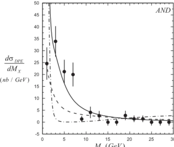
We start evaluating Eq. (18) with the inputs that were already fixed by other applications of the IGM, namely, (61) withpd = 0.05. In Fig. 13 we show the numerical results for DPE mass distribution normalized to the “AND” data sample of [24]. We have fixed the parameterσ(≡ σIP IP) appearing in Eq. (5) and Eq. (6), to0.5mb(dashed lines) and1.0mb(solid lines).

We emphasize that, in this approach, since we have fixed all parameters using previous data on leading particle for-mation and single diffractive mass spectra, there are no free parameters here, exceptσIP IP. As it can be seen from the figure, in our model we obtain the fast increase of spectra in the low mass region without the use of aMXdependentIP IP cross section and this quantity seems to be approximately σIP IP ≃0.5mb.

Figure 13. IGM DPE diffractive mass distributions: Solid and dashed lines show the results with σIP IP equal to 0.5mb and

1.0mb, respectively, calculated with the intermediate Pomeron profile. Our curves were normalized to the “AND” data sample of [24].

Figure 14. IGM DPE diffractive mass distributions: Solid line as in Fig. 13, dashed and dash-dotted lines represent the “hard” and “super-hard” Pomeron profiles. In all casesσIP IP = 0.5mb. Our

We next replace (61) by the convolution (60) to see which of the previously considered Pomeron profiles, hard or superhard, gives the best fit of the UA8 data. In doing so, we shall keep everything else the same, i.e.,pd = 0.05and σIP IP = 0.5mb.

In Fig. 14, we repeat the fitting procedure used in Fig. 13 for these Pomeron profiles. Solid, dashed and dash-dotted lines represent respectively Eq. (61), hard and superhard Pomerons. We see that, for harder Pomeron profiles we “dig a hole” in the low mass region of the spectrum. Note that the solid lines are the same as in Fig. 13. Looking at the figure, at first sight, we might be tempted to say that Eq. (61) gives the best agreement with data and a somewhat worse de-scription can be obtained with the hard Pomeron (in dashed lines), the superhard being discarded. However, compar-ing the dashed lines in Fig. 13 and Fig. 14 and observcompar-ing that they practically coincide with each other, we conclude that the same curve can be obtained either with (61) and σIP IP = 1.0mb(dashed line in Fig. 13) or with (60), (56) andσIP IP = 0.5mb(dashed line in Fig. 14).In other words we can trade the “hardness” of the Pomeron with its interac-tion cross secinterac-tion. The following two objects give an equally good description of data: i) a Pomeron composed by more and softer gluons and with a larger cross section and ii) a Pomeron made by fewer, harder gluons with a smaller inter-action cross section. We have checked that this reasoning can be extended to the superhard Pomeron. Although, ap-parently disfavoured by Fig. 14 (dash-dotted lines), it might still fit the data provided that σIP IP <0.25mb. Given the uncertainties in the data and the limitations of the model, we will not try for the moment to refine this analysis. It seems possible to describe data in a number of different ways. We conclude then that nothing exotic has been observed and also that the Pomeron-Pomeron cross section is bounded to beσIP IP <1.0mb.

Figure 15. IGM prediction fordσ/dMX at LHC withσIP IP =

1.0mb. Cross(+) and Cross(×) are predictions made by Brandt

et al. [24] for two values of effective Pomeron interceptsα(0) = 1 +ε.

In Fig. 15 we compare our predictions for dσ/dMX (mb/GeV) for LHC (√s = 14 TeV) assuming an MX

-independentσIP IP = 1.0mb(and using (61)) with predic-tions made by Brandtet al. [24] for two values of effective Pomeron intercepts (α(0) = 1 +ε),ε= 0.0and0.035.

Figure 16. Ratio double/single Pomeron exchange mass distri-butions as a function ofMX. In both cases we have assumed

σIP IP = 1.0mb(for DPE processes) andσpIP = 1.0mb(for SPE

processes).

Although the normalization of our curves is arbitrary, the comparison of the shapes reveals a difference between the two predictions. Whereas the points (from [24]) show spectra broadening with the c.m.s. energy, we predict (solid line) the opposite behavior: as the energy increases we ob-serve a (modest) narrowing fordσ/dMX. This small effect means that the diffractive mass becomes a smaller fraction of the available energy√s.In other words, the “double dif-fractive inelasticity” decreases with energy in the same way as the “diffractive inelasticity”, as seen in Fig. 10.

We are not able to make precise statements about the diffractive cross section (in particular about its normaliza-tion) with our simple model. Nevertheless, the narrowing of dσDP E/dMX suggests a slower increase (with√s) of the integrated distributionσDP E. We found this same ef-fect also forσSP E. This trend is welcome and is one of the possible mechanisms responsible for the suppression of diffractive cross sections at higher energies relative to some Regge theory predictions.

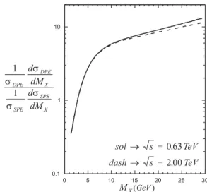
In Fig. 16 we show the ratioR(MX)defined by:

R(MX) = 1 σDP E

dσDP E

dMX

1 σSP E

dσSP E

dMX

(19)

This quantity involves only distributions previously normal-ized to unity and does not directly compare the cross sec-tions (which are numerically very different for DPE and sin-gle diffraction). InRthe dominant1/M2

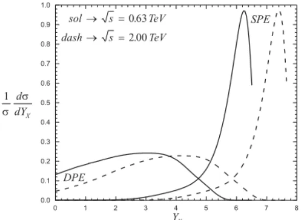
a consequence, when energy is released from the incoming particles in a SPE event, it goes more to kinetic energy of the X system (i.e., larger momentumPXand rapidityYX) and less to its mass. In DPE, although less energy is released, it goes predominantly to the massMXof the difractive cluster, which is then at lower values ofYX. In order to illustrate this behavior, we show in Fig. 17 the rapidity distributions of the X (which has massMX) andXY (which has massMXY) systems. All curves are normalized to unity and with them we just want to draw attention to the dramatically different positions of the maxima of these distributions. The solid and dashed lines show1/σ dσ/dYXfor DPE (curves on the left) and SPE (curves on the right) computed at√s= 630GeV and√s= 2000GeV, respectively. We can clearly observe that DPE and SPE rapidity distributions are separated by three units of rapidity and this difference stays nearly con-stant as the c.m.s. energy increases. The location of maxima in1/σ dσ/dYXand their energy dependence are predictions of our model.

Figure 17. Double and single Pomeron exchange normalized rapidity (YX) distributions. In both cases we have assumed

σIP IP = 1.0mb(for DPE processes) andσpIP = 1.0mb(for SPE

processes).

8

Leading particle spectra

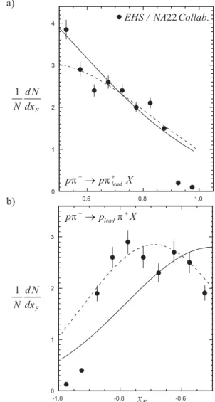
The leading particle effect is one of the most interesting features of multiparticle production in hadron-hadron colli-sions. In high energy hadron-hadron collisions the momen-tum spectra of outgoing particles which have the same quan-tum numbers as the incoming particles, also called leading particle (LP) spectra, have been measured already some time ago [60, 61]. Later on, new data on pion-proton collisions were released by the EHS/NA22 collaboration [62] in which the spectra of both outcoming leading particles, the pion and the proton, were simultaneously measured. More recently data on leading protons produced in eletron-proton reactions at HERA with a c.m.s. energy one order of magnitude higher than in the other above mentioned hadronic experiments be-came available [63]. In the case of photoproduction, data can be interpreted in terms of the Vector Dominance Model [64] and can therefore be considered as data on LP produc-tion in vector meson-proton collisions. These new measure-ments of LP spectra both in hadron-hadron and in eletron-proton collisions have renewed the interest on the subject,

specially because the latter are measured at higher energies and therefore the energy dependence of the LP spectra can now be determined.

It is important to have a very good understanding of these spectra for a number of reasons. They are the input for calculations of the LP spectra in hadron-nucleus colli-sions, which are a fundamental tool in the description of atmospheric cascades initiated by cosmic radiation [9, 65]. There are several new projects in cosmic ray physics includ-ing the High Resolution Fly’s Eye Project, the Telescope Array Project and the Pierre Auger Project [66] for which a precise knowledge of energy flow (LP spectra and inelas-ticity distributions) in very high energy collisions would be very useful.

In a very different scenario, namely in high energy heavy ion collisions at RHIC, it is very important to know where the outgoing (leading) baryons are located in momentum space. If the stopping is large they will stay in the cen-tral rapidity region and affect the dynamics there, generat-ing, for example, a baryon rich equation of state. Alterna-tively, if they populate the fragmentation region, the cen-tral (and presumably hot and dense) region will be domi-nated by mesonic degrees of freedom. The composition of the dense matter is therefore relevant for the study of quark gluon plasma formation [8].

In any case, before modellingp−AorA−Acollisions one has to understand properly hadron-hadron processes. The LP spectra are also interesting for the study of diffrac-tive reactions, which dominate the largexFregion.

Since LP spectra are measured in reactions with low mo-mentum transfer and go up to largexF values, it is clear that the processes in question occur in the non-perturbative do-main of QCD. One needs then “QCD inspired” models and the most popular are string models, like FRITIOF, VENUS or the Quark Gluon String Model (QGSM). Calculation of LP spectra involving these models can be found in Refs. [67] and [68].

8.1

Leading particles in hadron-hadron

colli-sions

models addressed these data and the conclusion was that va-lence quark recombination is needed. Translated to leading pion or proton production this means that what happens is rather a coalescence of valence quarks to form the LP and not an independent fragmentation of a quark or diquark to a pion or a nucleon.Another point is that the coherent con-figuration formed by the valence quarks may go through the target but, due to the strong stopping of the gluon clouds, may be significantly decelerated. This correlation between central energy deposition due to gluons and leading particle spectra was shown to be essential for the undertanding of leading charm production [14].

We follow the same general ideas of Ref. [67] but with a different implementation. In particular we replace indepen-dent fragmentation by valence quark recombination and free leading parton flow by deceleration due to “gluon stripping”. We have studied all measured LP spectra including those measured at HERA. We have found some universal aspects in the energy flow pattern of all these reactions. Universal-ity means, in the context of the IGM, that the underlying dy-namics is the same both in diffractive and non-diffractive LP production and both in hadron-hadron and photon-hadron processes.

In Ref. [17] we analyzed leading particle spectra in hadronic collisions and, assuming VDM, the leading proton spectra ine−preactions. We have also considered the con-tribution coming from the diffractive processes. The lead-ing particle can emerge from different regions of the phase space, according to the values assumed byxmaxandymax in eqs. (5) and (6). The distribution of its momentum frac-tionxLis given by:

F(xL) = (1−α)Fnd(xL) + j=1,2

αjFd(xL) (20)

whereα=α1+α2is the total fraction of single diffractive (d)events from the lower and upper legs in Fig. 1, respec-tively.

Notice thatαis essentially a new parameter here, which should be of the order of the ratio between the total diffrac-tive and total inelastic cross sections [15].

In Fig. 18 we present our spectra of leading protons, pi-ons and kapi-ons respectively. The dashed lines show the con-tribution of non-diffractive LP production and the solid lines show the effect of adding a diffractive component, calcu-lated with the intermediate Pomeron profile. All parame-ters were fixed previously and the only one to be fixed was α. For simplicity we have neglected the third diagram in Fig. 1(c), because it gives a curve which is very similar in shape to the non-diffractive curve. In contrast, the Pomeron emission by the projectile (Fig. 1b) produces the diffractive peak. We have then chosenα2= 0andα1=α= 0.3in all collision types.

As expected, the inclusion of the diffractive component flattens considerably the final LP distribution bringing it to a good agreement with the available experimental data [60, 61]. In our model there is some room for changes lead-ing to fits with better quality. We could, for example, use a prescription for hadronization (as we did before in [13])) giving a more important role to it, as done in Ref. [67]. In

Figure 18. Comparison of our LP spectraF(xL)with data from [61] and [60].

doing this, however, we loose simplicity and the trans-parency of the physical picture, which are the advantages of the IGM. We prefer to keep simplicity and concentrate on the interpretation of our results. In first place it is interesting to observe the good agreement between our curve and data for protons (Fig. 18a) in the lowxL region. The observed protons could have been also centrally produced, i.e., they could come from the CF. However we fit data without the CF contribution. This suggests, as expected, that all the protons in this xL range are leading, i.e., they come from valence quark recombination. In Figs. 18b) and 18c) we observe an excess at low xL. This is so because pions and kaons are light and they can more easily be created from the sea (centrally produced). Our distributions come only from the leading jet and consequently pass below the data points. A closer look into the three dashed lines in Fig. 18 shows that pion and kaon spectra are softer than the proton one. The former peak atx≃0.56while the latter peaks atx≃0.62.

In the IGM this can be understood as follows. The energy fraction that goes to the central fireball,K =√xy, is con-troled by the behaviour of the functionχ(x, y)nd_{, which is} approximately a double gaussian in the variablesxandy, as it can be seen in expression (1). The quantitiesxandy

play the role of central values of this gaussian. Consequently whenxoryincreases, this means that the energy depo-sition from the upper or lower leg (in Fig. 1) increases re-spectively. The quantitiesxandyare the moments of theωfunction and are directly proportional to the gluon dis-tribution functions in the projectile and target and inversely proportional to the target-projectile inelastic cross section. In the calculations, there are two changes when we go from

(i) The first is that we replace σ_inelpp by σ_inelπp which is smaller. This leads to an overall increase of the en-ergy deposition. There are some indications that this is really the case and the inelasticity inπ−pis larger than inp−pcollisions1.

(ii) The second and most important change is that we re-place one gluon distribution in the proton Gp_(y)by the corresponding distribution in the pionGπ(y). We know that Gp_{(y) ≃ (1−y)}5_{/y whereas G}π_{(y) ≃} (1−y)2_{/y, i.e., that gluons in pions are harder than} in protons. This introduces an asymmetry in the mo-ments x and y, making the latter significantly larger.

As a consequence, because of their harder gluon distrib-utions, pions will be more stopped and will emerge from the collision with a softerxLspectrum.This can already be seen in the data points of Fig. 18. However since these points con-tain particles produced by other mechanisms, such as central and diffractive production, it is not yet possible to draw firm conclusions. One should mention here that there is another possible difference between nucleons and mesons which can contribute to the different behaviour of the leading particles in both cases. It is connected with the triple gluon junction present in baryons but not in mesons, which, if treated as an elementary object, can influence sunbstantially LP spectra (cf. [71]). We shall not discuss this possibility in this paper. The analysis of the moments xand y can also be done for the diffractive process shown in Fig. 1b). Because of the cuts in the integrations in eq. (2), they will depend on xL = 1−y. We calculate them forp+p → p+X and π+p → π+X reactions. For lowxL they assume very similar values as in the non-diffractive case. For largexL however we find thatxp ≃ xπ andyp ≃ yπ. The reason for these approximate equalities is that in diffractive processes we cut the large y′ _{region and this is precisely} where the pion and the proton would differ, since only for largeyareGp_IP(y)≃(1−y)5_/yandGπ

IP(y)≃(1−y)2/y significantly different. In Ref. [15] we have shown that the introduction of the above metioned cuts drastically reduces the energy (√s) dependence of the diffractive mass distrib-utions leading, in particular, to the approximate1/M2

X be-haviour for all values of√sfrom ISR to Tevatron energies. Here these cuts produce another type of scaling, which may be called “projectile scaling” or “projectile universality of the diffractive peak” and which means that for large enough xLthe diffractive peak is the same for all projectiles. The correspondingχd_{functions will be the same for protons and} pions in this region. The cross section appearing in the de-nominator of the moments will, in this case, be the same, i.e.,σIP p_.

The only remaining difference between them, their dif-ferent gluonic distributions, is in this region cut off. This may be regarded as a prediction of the IGM. Experimen-tally this may be difficult to check since one would need a large number of points in largexLregion of the leading par-ticle spectrum. Data plotted in Fig. 18 neither prove nor

dis-prove this conjecture. The discrepancy observed in the pro-ton spectrum is only due to our choice of normalization of the diffractive and non-diffractive curves. The peak shapes are similar.

Figure 19. a) Comparison of our spectraF(xL)for leading pions

with data from Ref. [62] in the reactionπ+_+p

→π+_+p+X. Solid and dashed lines correspond to the choicesm0 = 0.35GeV andm0= 0.45GeV respectively. b) the same as a) for the leading proton spectrumF(xF)measured in the same reaction.

The EHS/NA22 collaboration provided us with data on π+_+p→π+_{+p+Xreactions. In particular they present} thexF distributions of both leading particles, the pion and the proton. Their points for pions and protons are shown in Fig. 19a) and b) respectively. These points are pre-sumably free from diffractive dissociation. The above men-tioned asymmetry in pion and proton energy loss emerges clearly, the pions being much slower. The proton distrib-ution peaks at xF ≃ 0.6−0.8. Our curves (solid lines) reproduce with no free parameter this behaviour and we ob-tain a good agreement with the pion spectrum. Proton data show an excess at largexF that we are not able to reproduce keeping the same values of parameters as before.

1_{For example, in the cosmic ray experiments it is usually assumed thatK}

The authors of Ref. [62] tried to fit their measured pro-ton spectrum with the FRITIOF code and could not obtain a good description of data. This indicates that these large xF points are a problem for standard multiparticle produc-tion models as well. In our case, if we change our parameter m0 from the usual value m0 = 0.35GeV (solid line) to m0 = 0.45GeV (dashed line) we can reproduce most of data points both for pions and protons as well. This is not a big change and indicates that the model would be able to accomodate this new experimental information. Of course, a definite statement about the subject would require a global refitting procedure, which is not our main concern now.

8.2

Leading particles in photon-proton

colli-sions

If, at high energies, the reactions ρ−p and π−p have the same characteristics and if VDM is a good hypothesis, then more about the energy flow in meson-pcollisions can be learned at HERA. Indeed, as mentioned in [54], at the HERA electron-proton collider the bulk of the cross sec-tion corresponds to photoproducsec-tion, in which a beam elec-tron is scattered through a very small angle and a quasi-real photon interacts with the proton. Using VDM, high energy photoproduction exhibits therefore similar characteristics to hadron-hadron interactions.

Data taken by the ZEUS collaboration at HERA [63] show that the LP spectra measured in photoproducion and in DIS (where Q2 _{≥ 4 GeV}2_{) are very similar, specially} in the largexLregion. This suggests that, as pointed out in [72], the QCD hardness scale for particle production in DIS gradually decreases from a (large)Q2_{, which is relevant in} the photon fragmentation region, to a soft scale in the proton fragmentation region, which is the one considered here. We can therefore expect a similarity of the inclusive spectra of the leading protons in high energy hadron-proton collisions, discussed above, and in virtual photon-proton collisions. In other words, we may say that the photon is neither resolv-ing nor beresolv-ing resolved by the fast emergresolv-ing protons. This implies that these reactions are dominated by some non-perturbative mechanism. This is confirmed by the failure of perturbative QCD [73], (implemented by the Monte Carlo codes ARIADNE and HERWIG) when applied to the pro-ton fragmentation region. In Ref. [72] the LP spectra were studied in the context of meson and Pomeron exchanges. Here we use the vector meson dominance hypothesis and describe leading proton production in the same way as done for hadron-hadron collisions. The only change is that now we haveρ−pinstead ofp−pcollisions. Whereas this may be generally true for photoproduction, it remains an approx-imation for DIS, valid in the largexLregion.

Assuming that VDM is correct, the incoming photon line can be replaced by solid line in Fig. 1. During the inter-action the photon is converted into a hadronic state, called V, and then interacts with the incoming proton. At HERA only collisionsV −pare relevant. The stateV looses frac-tionxof its original momentum and gets excited carrying a xF = 1−xfraction of the initial momentum. The proton, which we call here the diffracted proton, looses only a

frac-tiony of its momentum but otherwise remains intact. We assume here, for simplicity, that the vector meson is aρ0 and takeGρ0

(x) =Gπ_{(x)in eqs. (5) and (6).}

Figure 20. Comparison between our calculation and the data on the leading proton spectrum measured at HERA by the ZEUS Collab. [23].

In Fig. 20 we present our spectrum of leading protons inγp collisions. All parameters leading to the results in that figure are the same as established before in our study of diffractive mass distributions in photon-proton collision at HERA.

8.3

Leading

J/ψ

production

All produced particles come essentially from the gluons and quark-antiquark pairs already pre-existing in the projectile and target, or radiated during the collision. This qualitative picture takes different implementations in the many existing multiparticle production models. In the IGM, the produced particles (and consequently the energy released in the sec-ondaries and lost by the projectiles) come almost entirely from the pre-existing gluons in the incoming hadrons. This conjecture may be directly tested using a high energy, nearly gluonless hadronic projectile. In this case, according to the IGM, inspite of the high energy involved, the production of secondaries would be suppressed in comparison to the pro-duction observed in reactions induced by ordinary hadrons. The energy would be mostly carried away by the projectile leading particle which would then be observed with a hard xF spectrum. This type of gluonless projectile is available inJ/ψ photoproduction, where the photon can be under-stood as a virtualc¯cpair which reacts with the proton and turns into the finally observedJ/ψ. There are low energy data taken by the FTPS Collaboration [74] and high energy data from HERA [75].

Figure 21. Comparison of the IGM distributionF(z) with data of Ref. [75] with restricted acceptancep2

T ≥ 1 (GeV /c)

2 and

0.5≤ z ≤ 0.9for fixed value ofσinel

J/ψ−p = 9mband for three

different values ofpJ/ψ_{: 0.066(dashed line),0.033(solid line)}

and0.016(dotted line).

The crucial role played by the parameter p (see eq. (8)) representing the energy-momentum fraction of a given hadron allocated to gluons is best seen in Fig. 21 where we show the fit to data for leadingJ/ψphotoproduction [75]. The only parameter to which results are really sensitive is p=pJ/ψ _{which, as shown in Fig. 21, has to be very small,} pJ/ψ_{= 0.033. This is what could be expected from the fact} that charmonium is a non-relativistic system and almost all its mass comes from the quark masses leaving therefore only a small fraction,

pJ/ψ ₌ MJ/ψ−2mc MJ/ψ ≃

0.033, (21)

for gluons (heremc = 1.5GeV andMJ/ψ = 3.1GeV). Of course, the value ofpJ/ψ _{required to give a very good} fit of data might change either with another choice ofmc or another choice ofσinel

J/ψ−p. However these changes might affectpJ/ψ _{by, at most, a factor two.This suggests that the} momentum fraction carried by gluons in theJ/ψis one or-der of magnitude smaller than that carried by gluons in light hadrons.

9

Summary and conclusions

We were able to fit an impressive amount of experimental data, which had nothing in common except the fact that they always referred to the momentum (or rapidity) distribution of some observed particle or to the invariant mass distribu-tion of a cluster of measured particles. We could fit these data starting from one single ”generating” function,χ(x, y), which depends almost only on the density and interaction cross section of the gluons inside hadrons. These are fun-damental quantities in QCD and with our model we can test the existing results for them. More than just fitting, we did some predictions and one of them, the leading particle spec-trum shown in Fig. 20, was confirmed by experiment.

After all these works, we may ask ourselves what have we learned. We believe that we have constructed a sim-ple and consistent picture of energy flow in strong interac-tions, based on the assumption thatenergy loss and lead-ing particle spectra are determined by many independent

gluon-gluon collisions and valence quarks play a secondary role. Consequently, energy flow will reflect the properties of the gluon distributions and cross sections in the colliding hadrons. This picture seems to be universal, i.e., valid in many different contexts. However, in order to see this uni-versality we have to be careful and use proper kinematical limits of the phase space for every reaction considered, as illustrated in Figs. 1 and 2. When this is done the sensi-tivity of energy flow to other (than gluon distributions and cross sections) aspects of the production process is only of secondary importance and needs special observables (which are sensitive to, for example, the quantum numbers of the detected particles) to be visible. But even then, the IGM is indispensable because it provides the important energy cor-relations between different parts of the phase space.

Our analysis shows also clearly that our model can be regarded as a useful reference point for all more sophisti-cated approaches whereas, for hydrodynamical approaches of multiparticle production, it provides the initial energy used for the further evolution and hadronization of the cre-ated systems. However, in order to comply with the recent developments of QCD concerning the lowxgluonic con-tent of hadrons [26, 27] it must be accordingly updated. We plan to do this in the future. We also plan to account for the intrinsic fluctuations present in the hadronizing systems. In the usual statistical models this can be done by using the so called nonextensive statistics and, as was shown in [76], it can influence substantially some energy flow results, in particular the estimation of inelasticityK.

Appendix A

The main ideas

The IGM can be summarized in the following way: (i) The two colliding hadrons are represented by valence

quarks carrying their quantum numbers plus the ac-companying clouds of gluons.

(ii) In the course of a collision the gluonic clouds interact strongly depositing in the central region of the reac-tion fracreac-tionsxandy of the initial energy-momenta of the respective projectiles in the form of a gluonic Central Fireball(CF).

(iii) The valence quarks get excited and formLeading Jets (LJ’s) which decay and populate mainly the fragmen-tation regions of the reaction.

The fraction of energy stored in the CF is therefore equal toK = √xyand its rapidity isY = 1

2 ln x y.

and we assume that they coalesce forming the CF. The colli-sions leading to MF’s occur at different energy scales given byQ2

i =xiyis, where the indexilabels a particular kine-matic configuration where the gluon from the projectile has momentumxiand the gluon from the target hasyi. We have to choose the scale where we start to use perturbative QCD. Below this value we have to assume that we can still talk about individual soft gluons and due to the short correlation length between them they still interact mostly pairwise. In this region we can no longer use the distribution functions extracted from DIS nor the perturbative elementary cross sections.

The central formula

The central quantity in the IGM is the probability to form a CF carrying momentum fractionsxandyof two colliding hadrons. It is defined as the sum over an undefined number n of MF’s:

χ(x, y) = n1

n2 · · ·

ni

δ[x−n1x1− · · · −nixi]

× δ[y−n1y1− · · · −niyi]P(n1)· · ·P(ni)

=

{ni}

δ

x−

i nixi

δ

y−

i niyi

×

{ni}

P(ni) (22)

The delta functions in the above formula garantee en-ergy momentum conservation and P(ni) is the probabil-ity to have ni collisions between gluons with xi and yi. The expression above is quite general. It becomes specific when we defineP(ni). The assumption of multiple parton-parton incoherent scattering (which is also used in Refs. [1, 29, 30, 31, 34]) implies a Poissonian distribution of the number of parton-parton collisions and thusP(ni)is given by:

P(ni) = (ni) ni_exp(

−ni) ni!

(23)

InsertingP(ni)in (22) and using the following integral representations for the delta functions:

δ

x−

i nixi

= = 1 2π +∞ −∞ dtexp it x− i nixi

(24) δ y− i niyi

= = 1 2π +∞ −∞ du exp iu y− i niyi

(25)

we can perform all summations and products arriving at:

χ(x, y) = 1 (2π)2

+∞

−∞

dt

+∞

−∞

duexp [i(tx+uy)]

× exp i ni

e−i(txi+uyi)

−1

(26)

Taking now the continuum limit: ni = dni

dx′_dy′∆x′∆y′ −→ dn =

dn

dx′_dy′dx′dy′ (27) we obtain:

χ(x, y) = 1 (2π)2

+∞

−∞

dt

+∞

−∞

du exp[i(tx+uy)]

× exp 1 0 dx′ 1 0

dy′ω(x′, y′)e−i(tx′+uy′)−1

(28) where

ω(x′, y′) = dn

dx′_dy′. (29) This functionω(x′_{, y}′_{)is called the spectral function and} represents the average number of gluon-gluon collisions as a function ofx′_ey′_{. It contains all the dynamical inputs of} the model and has the form:

ω(x′, y′) = σgg(x′y′s) σ(s) G(x

′_)G(y′₎

× θ

x′y′−Kmin2

, (30) whereG’s denote the gluon distribution functions in the cor-responding projectiles and σgg andσ are the gluon-gluon and hadron-hadron cross sections, respectively. In the above expressionx′_andy′_{are the fractional momenta of two} glu-ons coming from the projectile and from the target whereas Kmin = m0/√s, withm0being the mass of lightest pro-duced state and√sthe total c.m.s. energy.m0is a parame-ter of the model.

The integral in the second line of eq. (28) is dominated by the lowx′ _andy′ _{region. Considering the singular} be-havior of theG(x)distributions at the origin we make the following approximation:

e−i(tx′+uy′)−1 ≃ −i(tx′+uy′)−1₂(tx′+uy′)2 (31) With this approximation it is possible to perform the in-tegrations in (28) and obtain the final expression forχ(x, y) discussed in the main text:

χ(x, y) = χ0 2π

Dxy

exp{−_2D1

xy[y 2

(x− x)2

+ x2_{(y− y)}2_{+ 2xy(x− x) (y− y)]}(32)} where