Article
J. Braz. Chem. Soc., Vol. 27, No. 1, 84-90, 2016. Printed in Brazil - ©2016 Sociedade Brasileira de Química 0103 - 5053 $6.00+0.00
A
*e-mail: [email protected]
Qualitative and Quantitative Monitoring of Methyl Cotton Biodiesel Content in
Biodiesel/Diesel Blends Using MIR Spectroscopy and Chemometrics Tools
José Eduardo Buiatte,a Eloíza Guimarães,a Hery Mitsutake,a Lucas Caixeta Gontijo,*,a,b
Douglas Queiroz Santosc and Waldomiro Borges Netoa
aInstituto de Química, Universidade Federal de Uberlândia, Campus Santa Mônica,
38408-100 Uberlândia-MG, Brazil
bInstituto Federal Goiano de Educação, Ciência e Tecnologia, 75790-000 Urutaí-GO, Brazil
cEscola Técnica de Saúde, Universidade Federal de Uberlândia, Campus Umuarama,
38400-902 Uberlândia-MG, Brazil
This paper presents methodologies for monitoring the quality of methyl cotton biodiesel in biodiesel/diesel blends using mid-infrared spectroscopy (MIR) and chemometrics tools. The first method relates to the construction of multivariate control charts with the aim of qualitatively monitoring the samples according to the Brazilian specification for biodiesel in the biodiesel/diesel blends (7.00 ± 0.5% v/v of biodiesel). The second concerns the construction of partial least squares (PLS) to determine the content of the biodiesel in the biodiesel/diesel blend. The PLS model was validated from multivariate figures of merit according to the guidelines of ASTM E1655-05 and IUPAC. The results from both methods were satisfactory for both qualitative and quantitative monitoring. Therefore, the proposed methodologies for monitoring the quality of biodiesel in biodiesel/diesel blends are fast, practical, economical and efficient and can be used by industries and service stations.
Keywords: biodiesel, mid-infrared spectroscopy, chemometrics tools, multivariate control charts, PLS
Introduction
The search for alternatives to oil use increases the
importance of commercial production of biofuels.1 Among
the biofuels, biodiesel has stood out for being a renewable fuel derived from vegetable oils, animal fats or waste, and can be a total or partial surrogate of mineral diesel.
Thus, in 2005, this fuel was introduced to the Brazilian
energy matrix2 and the addition of 7% (v/v) to diesel oil has
now become mandatory.3 Therefore, due to the requirement
of this blend, analytical control of the biodiesel content blended with diesel is critical. Biodiesel production in Brazil can use various feedstocks (any oilseed and animal fats) and various alcohols (usually methanol or ethanol), provided that the final product meets the specifications of the National Agency of Petroleum, Natural Gas and
Biofuels (ANP).4 Thus, the choice of raw material depends
on the availability, cost and production technology. 5 In this
perspective, considering that about 50-90% of biodiesel production costs is due to the raw material used, the use of oils derived from waste has been excelled, as this decreases
the cost of production.6,7 Therefore, cottonseed oil becomes
a viable oilseed because it is a waste of cotton production. Moreover, it is the third most commonly used raw material in biodiesel production in Brazil and the country is the fifth
largest producer of cotton.8
Diverse methodologies for the study of the quality of biodiesel in biodiesel/diesel blend are designed, involving various techniques and combined with some types of chemometric tools. Among such techniques are near
infrared spectroscopy (NIR)9 and mid-infrared spectroscopy
(MIR),10,11 high-performance liquid chromatography
(HPLC),12 mass spectrometry with electrospray ionization
(ESI-MS)13 and others.14,15 However, most studies have been
squares (PLS) methodologies from MIR spectroscopy data have been found.
In this context, this paper presents multivariate methodologies for the identification and quantification of methyl cotton biodiesel content in biodiesel/diesel blends using mid-infrared spectroscopy.
Brief description of multivariate control charts based on NAS
Control charts consists of charts that monitor some important feature of a quality control process. The charts based on net analytical signal (NAS) allow separate control, but simultaneous analysis of the quality of the analyte of interest and its mother, who is not modeled by either of
these two (noise/waste).16
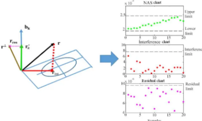
The basis for the development of control charts is
shown in Figure 1, in which a sample spectrum (vector r)
is divided into three different contributions: the NAS vector
(rNAS) for monitoring the analyte of interest, the interference
vector (rint) and the residual vector (rres). The contributions
related to the analyte of interest (biodiesel in the case of this study) are modeled by the NAS vector; the contributions of the matrix (diesel) are modeled by interference vector and the contributions that were not modeled by NAS and
interference vectors correspond to the residual vector.17
From the statistical limits calculated for each contribution/ vector, it is possible to determine whether a sample is within the quality compliance or not. Thus, a sample is considered under control, i.e., within quality specifications, if it is within all the calculated limits; otherwise, if it protrudes from at least one of the thresholds, the sample is considered out the quality specifications (out of control). Limits of NAS chart are calculated from the standard deviation of the mean NAS and the 95% confidence limit. The interference projection vectors are calculated for the spectra of the interfering area, as shown in Figure 1. The distance of this projection relative to the ellipse center provides the
distance value D, which is used to compute the threshold of the interference chart 95% reliability. The limits of the
residual chart are calculated based on the χ2 statistics of
the sum of squares of the residual vector of the calibration
samples.16 The equations for calculating the boundaries of
three charts can be found in the literature.16-18
Brief description of PLS
Partial least squares regression (PLS) is a chemometric tool that is widely used in multivariate calibration in various fields of science. In the PLS modeling, both the matrix
of independent variables X and the dependent variables
Y are represented by scores and weights according to
equations 1 and 2.
X = TPt + E (1)
Y = UQt + F (2)
where X is the matrix of data (measurement instrument),
Y is the vector response (concentration, for example), T
and U are the scores for the two data matrices, P and Q are
the respective weights, E and F are the respective residues,
or matrices containing the part that is not modeled. The
relationship between the two data arrays X and Y can be
obtained by correlating the scores of each block, to obtain a linear relationship described in equation 3.
U = bT + eE (3)
where U is a matrix containing the properties of all samples
(in this case, the concentration), b is a vector containing
the model parameters, T is a response matrix (spectra) for
the calibration samples, and E is a matrix representing the
spectrum of the noise and model errors.19
In this process, the choice of the number of latent variables is necessary, which is usually done by using a so-called cross-validation procedure based on the lowest prediction error. Evaluating the reliability of the constructed model for the
validation can be done according to ASTM E1655-0520 or
by figures of merit such as: accuracy, linearity, selectivity, sensitivity, analytical sensitivity, limit of detection, limit of quantification, signal to noise ratio, and test to systematic error (bias), including confidence ellipse.
Experimental
Biodiesel production
Ten lots of diesel-free biodiesel used in sample preparation was ceded by Transpetro S/A. The cottonseed
Figure 1. The instrumental signal decomposition in three different
contributions: NAS vector (rNAS) for monitoring the analyte of interest,
oil, used in the biodiesel synthesis was acquired by Triângulo Alimentos S/A industry. To obtain biodiesel, 30 g of methyl alcohol, 1 g of KOH and 100 g of oil in a molar ratio (1:6) were used. Methyl alcohol-KOH manual agitation was used until complete homogenization, forming the potassium methoxide. The oil was added to the methoxide for 80 min at room temperature and stirred using a magnetic stirrer. At the end of the reaction, there was phase separation in which the glycerin was removed and the biodiesel was washed with hot water to remove impurities. The biodiesel drying step was carried out using a rotary evaporator for 1 h at 78 rpm and 80°C.
Sample preparation
For the construction of control charts, the following samples divided into five sets were prepared, I: 10 diesel samples free of biodiesel; II: 20 samples under control (6.5-7.5%, v/v) used in the calibration set which were used to determine the limits of statistical control charts (this variation of concentration was chosen due to variation in the
volume allowed by Resolution 50 ANP,21 i.e., 0.5% v/v the
percentage of biodiesel in the blend); III:10 samples under
control (6.5-7.5%, v/v) used in the validation set, we used to determine the statistical limits of the charts; IV: 16 biodiesel samples whose concentrations are below the allowed and ranged from 0.5 to 6.0% (v/v); V: 12 samples with biodiesel content is above specified and varied 8.0-14.0% (v/v). The weight measurements were performed on an analytical balance (Sartorius, BP211D model). The solutions were homogenized on a vortex shaker (Phoenix, AP56 model). From the weight and density values of biodiesel and diesel the volume/volume relations were determined. In the construction of the PLS model, samples were prepared by adding biodiesel to ten lots of diesel fuel in a concentration range of 1.00% to 30.00% (v/v). Samples concentrations of 1 to 10% (v/v) were prepared in increments of 0.25%, 10 to 25% (v/v) in increments of 0.75% and after 25% (end of calibration curve) increments of 0.25% (v/v). The samples used for calibration (46 samples) and prediction (27 samples) were prepared on the model so that the prediction concentrations were different concentrations of the calibration.
Acquisition of spectral data
The MIR spectra were obtained in five replications in
the region of 4000 cm-1 to 600 cm-1 using the SpectrumTwo
model spectrometer (Perkin Elmer) with the horizontal attenuated total reflectance (HATR) ZnSe crystal attachment (Pike Techonologies). Control charts for the pre-processing
of data were made by first derivative. For the PLS model, baseline treatment was applied by the baseline function in
the regions 1850-2570 cm-1 and 3200-4000 cm-1. To execute
the multivariate procedures, MATLAB software version 6.1 (Mathworks Inc.) and PLS_Toolbox, version 3.5 (Eigenvector Research) were used.
Results and Discussion
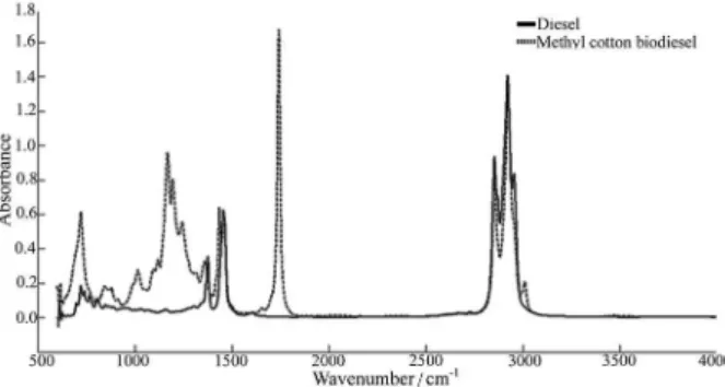
Figure 2 shows the MIR spectra of diesel and methyl cotton biodiesel. The diesel spectrum has substantial absorption bands corresponding to characteristic vibrational modes of normal alkanes. There are three significant
absorption spectral regions: (i) the region between 2840 cm-1
and 3000 cm-1 attributed to axial deformation vibration of
C–H bond of methyl and methylene groups; (ii) intermediate
intensity bands in the region of 1300 cm-1 to 1500 cm-1
derived from the angular deformation vibration of the C–H
bond of methylene and methyl group; and (iii) low intensity
band, which is relevant in the region of 720 cm-1, resulting
from the asymmetric angular deformation vibration of C–H deformations of methylene grouping. When analyzing the spectrum of biodiesel, in addition to the characteristic vibrational modes of methyl groups and methylene, two
strong bands are observed: (i) stretching of C=O bonds in
the region 1700 cm-1 to 1750 cm-1 and (ii) axial vibrations in
the region of C=O bond 1100 cm-1 to 1300 cm-1.22
For control charts, various mathematical treatments were tested. The best result was obtained using the first derivative because showed better performance in the correct classification of samples. The derivative was performed to remove baseline effects and to emphasize the spectral differences in each sample. The intervening space was built from the decomposition by principal component analysis (PCA) of the spectra of 10 samples of pure diesel (group I). Three principal components (PC) were chosen, which explained 100.00% of the variance. The statistical limits were calculated from the vectors NAS, interference
and residual, arising from the decomposition of the spectra of the calibration samples (group II).
It can be observed in Figure 3 that the most intense signals is the interference vector (diesel) for being the largest percentage component in the blend, i.e., much higher than the concentration of the analyte of interest, biodiesel. The regions in which the NAS vectors have higher intensities than the interference vectors are in
1760-1730 cm-1 and 1000-1300 cm-1. These regions refer to
absorptions due to C=O and C–O bands stretching present in the biodiesel, respectively. Moreover, it is observed that the residual vectors have low intensity demonstrating that small amount of the spectral signal is not modeled by the NAS and interference vectors.
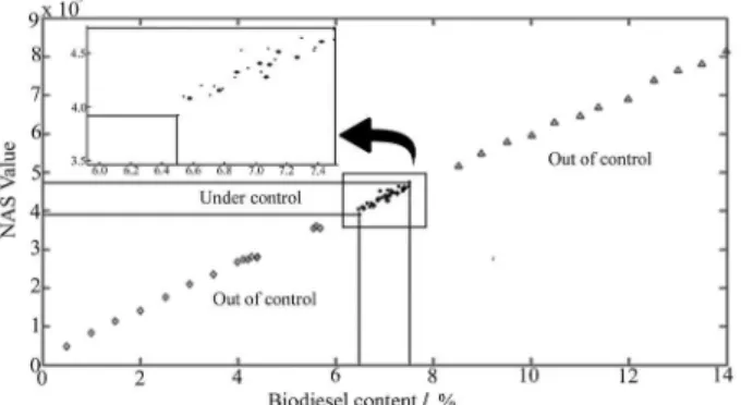
The vector NAS (biodiesel) is directly proportional to analyte concentration. Figure 4 shows the NAS vector in relation to the percentage of biodiesel in samples under control (groups II and III) and out of control (group IV: content below 6.5% and group V: content above 7.5%). The good linearity observed in Figure 4 demonstrates the linear relationship between the NAS vector and the concentration of biodiesel.
After the spectral decomposition step, the confidence limits were calculated for each chart using only samples
under control. The upper limit (NASsuperior) was 0.0048
and the lower (NASinferior) was 0.0039. The limits obtained
for interference chart (Dlimit,95% = 10.8597), showed values
higher than those found for the other charts. This is because these vectors have a much higher intensity than the NAS
vectors. In relation to the residual limit (Qα), the value found
was 4.4733 × 10⁻⁵, considering that this determination was
from samples under control, and that these samples that are not modeled by NAS and interference vectors are very small spectral parts, it was expected that the limits found for these charts were much lower than those found for the NAS and interference charts.
Figure 5 shows the control charts obtained for the calibration (group II) and validation (group III) samples. The first sample of the calibration set was erroneously classified as out of control because it came out of limit of residual chart. A possible explanation for this is that may have occurred an unexpected variation in the spectrometer signal or even an error in the preparation of this sample. However, all other samples were considered correctly as under control.
Figure 6 shows the multivariate control chart for the samples out of control because they have less than 6.5% (group IV) and more than 7.5% (group V) of biodiesel. The group IV values were below the lower limit, while
Figure 3. Intensity of NAS, interference and residual vectors obtained
from the calibration samples.
Figure 4. Relationship between the NAS vector and biodiesel
concentration. () group II (calibration set: under control); (*) group III (validation set: under control); () group IV and () group V: out of control samples.
Figure 5. Multivariate control chart for the samples under control, where
() group II and (*) group III.
group V samples show NAS values above the upper limits, as expected due to the property of the NAS to be proportional to the concentration of the analyte of interest in the sample. Thus, all samples of groups IV and V were properly monitored as out of control, demonstrating that this methodology is effective for the monitoring of quality biodiesel in biodiesel/diesel blends.
The PLS model was built using three latent variables which explained 99.96% and 99.99% of the variance of
blocks X and Y, respectively. The presence of outlier
was evaluated by Q residuals versus leverage, and it was
found that no sample was considered an outlier. After this evaluation, it was shown that the number of samples used in the construction of the PLS model was in accordance
with the guidelines of ASTM E1655-05.20
The fit of the model (Figure 7a) was evaluated by correlating the reference values and the values calculated by the model of the calibration and prediction sets. It was found that both sets (calibration and validation) showed low dispersion with respect to the expected values, i.e., regression coefficient (R) greater than 0.99. However, the value of R alone was not sufficient to confirm linearity, meaning that it is also necessary to analyze the plot of residuals for calibration and prediction samples. Thus, the Figure 7b shows that the proposed models exhibit linear behavior, since the distribution of residuals follows a random pattern.
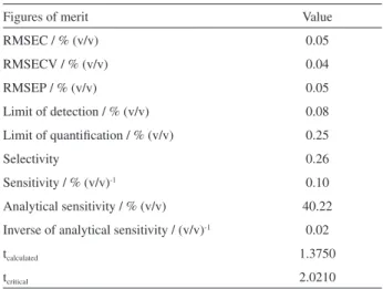
Table 1 shows the results of figures of merit for the PLS model. The accuracy of the model was evaluated in terms of root mean square error of calibration (RMSEC),
root meansquare error of cross validation (RMSECV) and
root mean square error of prediction (RMSEP). Low error values indicate that the values estimated by the PLS model have good agreement with the reference values. The model also has a value of RMSEP below 0.1%, which is within
the allowed by the standard NBR 15568.23
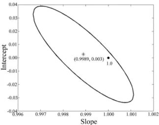
However, the evaluation of the model accurately from just the RMSEP value comprises all kinds of errors, both systematic and random. Thus, another way to compare the actual values and the predicted values is from the elliptical joint confidence region (EJCR) with respect to intercept and slope obtained from the regression of actual and projected values. Thus, it is observed in Figure 8 the point (1.0) lies inside the EJCR showing that the actual and predicted values do not present a significant difference with 95% confidence, that is, the absence of systematic
errors.24,25
The presence of systematic errors was also evaluated
according to the t test described by ASTM E1655-05.20
The results in Table 1 show that the calculated value t (tcalculated = 1.3750) is smaller than the critical value
(tcritical = 2.0210) with 95% confidence, which indicates that
the influence of the systematic errors can be negligible, i.e., the values predicted by the PLS model essentially provide
the same average result as the actual values.20
Figure 7. In(a) fit of the PLS models through the real versus predicted values of the prediction set. In (b) PLS residuals for the calibration and prediction set for the methyl cotton biodiesel in biodiesel/diesel blends.
Table 1. Results of the parameters of figures of merit for the PLS model
Figures of merit Value
RMSEC / % (v/v) 0.05
RMSECV / % (v/v) 0.04
RMSEP / % (v/v) 0.05
Limit of detection / % (v/v) 0.08
Limit of quantification / % (v/v) 0.25
Selectivity 0.26
Sensitivity / % (v/v)-1 0.10
Analytical sensitivity / % (v/v) 40.22
Inverse of analytical sensitivity / (v/v)-1 0.02
tcalculated 1.3750
Sensitivity was estimated as 0.10% (v/v)-1 (Table 1).
This parameter expresses an increase in the signal fraction when the concentration of the analyte of interest has a high
value for one unit.26 The inverse of the analytical sensitivity
value, shown in Table 1, can be interpreted more clearly because of the direct relationship with the concentration. According to this value, the PLS model is able to distinguish differences among samples with concentration in the range of 0.02% (v/v).
The selectivity parameter had a value of 0.26, indicating a significant overlap of the interfering signal with the analyte. However, unlike the univariate methods where there is a need for highly selective methods to perform the analysis, multivariate methods are employed in the construction of models from non-selective signals, where the application
effectively selects information extracted from these data.27
Moreover, a major advantage of the PLS is its ability to determine the analyte of interest, even in the presence of interferents, since these are present in the calibration.
By evaluating the limit of detection and the limit of quantification of the PLS model (Table 1), it was verified that the PLS model could detect amounts of biodiesel in diesel above 0.08% (m/m), while for the quantification, the model could not determine values lower than 0.25% (m/m). As the concentration of biodiesel in the proposed PLS model ranges from 1.00% to 30.00% (m/m), the model is effective at detecting and quantifying biodiesels in diesel blends at concentrations higher than 0.25% (m/m).
Conclusion
The methodology developed from MIR spectroscopy data combined with chemometric tools enables the monitoring of
methyl cotton biodiesel content in both the qualitative and quantitative aspects. Control charts can improve the quality of diagnoses, once out of control samples are easily identified in relation to the amount of biodiesel in the blend. It is simple, fast and can be developed for on-line monitoring sensors, requiring only the MIR spectra of samples under control and blank samples to build the charts. The development of the PLS model derived from data MIR blends of biodiesel/diesel fuel was also successful, indicating that the methodology can be applied to the quantification of methyl cotton biodiesel blended with diesel in the range of 1.00 to 30.00% (v/v). Validation of the PLS model was performed according to ASTM E1655 and Brazilian and international validation guides. The model developed is simpler than that proposed by ABNT NBR 15568, with the creation of a single curve for the concentration range of 1.00 to 30.00% (v/v) and without the use of solvents, as well as being within the error permitted by this standard. Therefore, regulators and supervisory bodies to control the biodiesel content in blends with diesel can use this methodology.
Acknowledgements
The authors would like to thank CAPES and FAPEG for their financial support and Caramuru S/A and Transpetro S/A for supplying the samples of the fuel.
References
1. The United States Pharmacopeia, USP 34-NF 29, The United States Pharmacopeial Convention: Rockville, 2011.
1. Kwon, E. E.; Jeon, E. C.; Yi, H.; Kim, S.; Appl. Energy 2014,
116, 20.
2. Ministério de Minas e Energia, Lei No. 11097, Diário Oficial da União: Brasília, 2005.
3. Ministério de Minas e Energia, Lei No. 13033, Diário Oficial da União: Brasília, 2014.
4. National Agency of Petroleum, Natural Gas and Biofuels;
Resolution ANP No. 14; Diário Oficial da União: Brasília, 2012.
5. Pinho, D. M. M.; Santos, V. O.; dos Santos, V. M. L.; Oliveira, M. C. S.; da Silva, M. T.; Piza, P. G. T.; Pinto, A. C.; Rezende, M. J. C.; Suarez, P. A. Z.; Fuel 2014, 136, 136.
6. Huang, Y. P.; Chang, J. I.; Renewable Energy2010, 35, 269. 7. Joshi, H.; Moser, B. R.; Walker, T.; J. Am. Oil Chem. Soc. 2011,
89, 145.
8. Associação Brasileira dos Produtores de Algodão; Report 2014. Available at: http://www.abrapa.com.br/estatisticas/Paginas/ Algodao-no-Brasil.aspx accessed in September 2015. 9. Balabin, R. M.; Safieva, R. Z.; Anal. Chim. Acta2011, 689, 190. 10. Gontijo, L. C.; Guimarães, E.; Mitsutake, H.; de Santana, F. B.;
Santos, D. Q.; Borges Neto, W.; Fuel2014, 117, 1111.
Figure 8. The elliptical joint confidence region (EJCR) for the slope
11. Mazivila, S. J.; de Santana, F. B.; Mitsutake, H.; Gontijo, L. C.; Santos, D. Q.; Borges Neto, W.; Fuel2015, 142, 222. 12. Brandão, L. F. P.; Braga, J. W. B.; Suarez, P. A. Z.;
J. Chromatogr. A2012, 1225, 150.
13. Eide, I.; Zahlsen, K.; Energy Fuel 2007, 21, 3702.
14. Corgozinho, C. N.; Pasa, V. M.; Barbeira, P. J.; Talanta 2008, 76, 479.
15. Meira, M.; Quintella, C. M.; Tanajura, A. S.; da Silva, H. R. G.; Fernando, J. D. S.; da Costa Neto, P. R.; Pepe, I. M.; Santos, M. A.; Nascimento, L. L.; Talanta2011, 85, 430.
16. Skibsted, E. T. S.; Boelens, H. F. M.; Westerhuis, J. A.; Smilde, A. K.; Broad, N. W.; Rees, D. R.; Witte, D. T.; Anal. Chem. 2005, 77, 7103.
17. de Oliveira, I. K.; Rocha, W. F. C.; Poppi, R. J.; Anal. Chim. Acta 2009, 642, 217.
18. Rocha, W. F. C.; Poppi, R. J.; Microchem. J. 2010, 96, 21. 19. Vandeginste, B. G. M.; Massart, D. L.; Buydens, L. M. C.;
Jong, S.; Lewi, P. J.; Smeyers-Verbeke, J.; Handbook of Chemometrics and Qualimetrics: Part B, 1st ed.; Elsevier
Science: Amsterdam, 1988.
20. ASTM E1655: Standard Practices for Infrared Multivariate Quantitative Analysis, West Conshohocken, 2005.
21. National Agency of Petroleum, Natural Gas and Biofuels;
Resolution No. 50; Diário Oficial da União: Brasília, 2013.
22. Holler, F. J.; Skoog, D. A.; Crouch, S. R.; Princípios de Análise Instrumental, 6ª ed.; Bookman: Porto Alegre, 2002.
23. ABNT NBR 15568: Biodiesel: Determination of Biodiesel Content in Diesel Oil via Mid-Infrared Spectroscopy; ABNT:
Rio de Janeiro, 2008.
24. de Souza, L. M.; Mitsutake, H.; Gontijo, L. C.; Borges Neto, W.;
Fuel2014, 130, 257.
25. Valderrama, P.; Braga, J. W. B.; Poppi, R. J.; J. Agr. Food. Chem. 2007, 55, 8331.
26. Valderrama, P.; Braga, J. W. B.; Poppi, R. J.; Quim. Nova2009,
32, 1278.
27. Olivieri, A. C.; Faber, N. M.; Ferré, J.; Boqué, R.; Kalivas, J. H.; Mark, H.; Pure Appl. Chem. 2006, 78, 633.
Submitted: June 23, 2015