Jeremias da Silva Leão

Saunders distribution for survival data

PROGRAMA INTERINSTITUCIONAL DE PÓS-GRADUAÇÃO EM ESTATÍSTICA UFSCar – USP

Jeremias da Silva Leão

Modeling based on a reparameterized

Birnbaum-Saunders distribution for analysis of survival data

Doctoral dissertation submitted to the Departamento de Estatística – Des/UFSCar and to Instituto de Ciências Matemáticas e de Computação – ICMC-USP, in partial fulfillmente of the requirements for the degree of the Doctorate in Statistics – Programa Interinstitucional de Pós-Graduação em Estatística UFSCar – USP.

Advisor: Prof. Dra. Vera Lucia Damasceno Tomazella

Co-advisor: Prof. Dr. Victor Eliseo Leiva Sanchez

UNIVERSIDADE FEDERAL DE SÃO CARLOS CENTRO DE CIÊNCIAS EXATAS E TECNOLOGIA

PROGRAMA INTERINSTITUCIONAL DE PÓS-GRADUAÇÃO EM ESTATÍSTICA UFSCar – USP

Jeremias da Silva Leão

Modelagem baseada na distribuição

Birnbaum-Saunders reparametrizada para análise de dados de

sobrevivência

Tese apresentada ao Departamento de Estatística – Des/UFSCar e ao Instituto de Ciências Matemáticas e de Computação – ICMC – USP, como parte dos requisitos para obtenção do título de Mestre ou Doutor em Estatística – Programa Interinstitucional de Pós-Graduação em Estatística UFSCar – USP.

Orientador: Prof. Dra. Vera Lucia Damasceno Tomazella

Co-orientador: Prof. Dr. Victor Eliseo Leiva Sanchez

L437m

Leão, Jeremias da Silva

Modeling based on a reparameterized Birnbaum-Saunders distribution for analysis of survival data / Jeremias da Silva Leão. -- São Carlos : UFSCar, 2017.

117 p.

Tese (Doutorado) -- Universidade Federal de São Carlos, 2017.

ACKNOWLEDGEMENTS

This work could never have been completed without ample guidance, assistance and encouragement. In this respect, I would like to thank the following persons:

My supervisors Prof. Vera Tomazella and Prof. Victor Leiva for their patience, encour-agement and guidance. I am indeed fortunate to learn from scholars of your calibre.

A special word of thanks to Helton Saulo for all the contribution during the development of the thesis.

The Departament of Statistics at UFSCar and USP.

The UFSCar/USP community, Isabel, Victor, Gláucia, Humberto and unknown servants, for support.

My UFSCar/USP friends, especially Edgar, José Clelto, Roberta, Daiane, Mauro, Pedro Ramos, Rafael Paixão, David and Andrey.

My professors Francisco Cysneiros, Leandro Rêgo, Maurício Motta, Luis Ernesto, Galvão, Vicente and Rafael Stern, for sharing some of your knowledge.

My UFPI friends, Máx, Valmária, Fernando, Cleide and Roney for the support when I left the institution.

My UFAM friends, Cardoso, James, Amazoneida, Joceli, José Raimundo and others for their support in my release to complete the doctorate degree.

My old friends, Hemílio, Josimar, Lutemberg, Marcelo, Manoel and William Marciano for unceasing friendship.

I would like to express my sincere thanks and gratitude to my parents, Antonia and Pedro, for all effort you put in my education. Thank you for your love and support. Also to my brother Paulo and my sister Miria as well as to my niece Ingrid and my sister-in-law Elizandra.

My wife, Themis and my daughters Lívia and Laís. Thank you for your love and companionship.

The committee members, my profound thanks.

“ A vida é o dever que nós trouxemos para fazer em casa.

Quando se vê, já são seis horas!

Quando de vê, já é sexta-feira!

Quando se vê, já é natal...

Quando se vê, já terminou o ano... Quando se vê perdemos o amor da nossa vida.

Quando se vê passaram 50 anos!

Agora é tarde demais para ser reprovado...

Se me fosse dado um dia, outra oportunidade, eu nem olhava o relógio.

Seguiria sempre em frente e iria jogando pelo caminho a casca dourada e inútil das horas...

Seguraria o amor que está a minha frente e diria que eu o amo...

E tem mais: não deixe de fazer algo de que gosta devido à falta de tempo.

Não deixe de ter pessoas ao seu lado por puro medo de ser feliz.

RESUMO

LEÃO, J. S.. Modeling based on a reparameterized Birnbaum-Saunders distribution for analysis of survival data. 2017. 117 f. Doctoral dissertation (Doctorate Candidate joint

Graduate Program in Statistics DEs-UFSCar/ICMC-USP) – Instituto de Ciências Matemáticas e de Computação (ICMC/USP), São Carlos – SP.

Nesta tese propomos modelos baseados na distribuição Birnbaum-Saunders reparametrizada introduzida por Santos-Neto et al. (2012) e Santos-Neto et al. (2014), para análise dados de sobrevivência. Incialmente propomos o modelo de fragilidade Birnbaum-Saunders sem e com covariáveis observáveis. O modelo de fragilidade é caracterizado pela utilização de um efeito aleatório, ou seja, de uma variável aleatória não observável, que representa as informações que não podem ou não foram observadas tais como fatores ambientais ou genéticos, como também, informações que, por algum motivo, não foram consideradas no planejamento do estudo. O efeito aleatório (a “fragilidade”) é introduzido na função de risco de base para controlar a heterogeneidade não observável. Usamos o método de máxima verossimilhança para estimar os parâmetros do modelo. Avaliamos o desempenho dos estimadores sob diferentes percentuais de censura via estudo de simulações de Monte Carlo. Considerando variáveis regressoras, derivamos medidas de diagnóstico de influência. Os métodos de diagnóstico têm sido ferramentas importantes na análise de regressão para detectar anomalias, tais como quebra das pressuposições nos erros, presença de outliers e observações influentes. Em seguida propomos o modelo de fração de cura com fragilidade Birnbaum-Saunders. Os modelos para dados de sobrevivência com proporção de curados (também conhecidos como modelos de taxa de cura ou modelos de sobrevivência com longa duração) têm sido amplamente estudados. Uma vantagem importante do modelo proposto é a possibilidade de considerar conjuntamente a heterogeneidade entre os pacientes por suas fragilidades e a presença de uma fração curada. As estimativas dos parâmetros do modelo foram obtidas via máxima verossimilhança, medidas de influência e diagnóstico foram desenvolvidas para o modelo proposto. Por fim, avaliamos a distribuição bivariada Birnbaum-Saunders baseada na média, como também introduzimos um modelo de regressão para o modelo proposto. Utilizamos os métodos de máxima verossimilhança e método dos momentos modificados, para estimar os parâmetros do modelo. Avaliamos o desempenho dos estimadores via estudo de simulações de Monte Carlo. Aplicações a conjuntos de dados reais ilustram as potencialidades dos modelos abordados.

Palavras-chave: Análise de diagnóstico, Distribuição Birnbaum-Saunders, Estimação de

ABSTRACT

LEÃO, J. S.. Modeling based on a reparameterized Birnbaum-Saunders distribution for analysis of survival data. 2017. 117 f. Doctoral dissertation (Doctorate Candidate joint

Graduate Program in Statistics DEs-UFSCar/ICMC-USP) – Instituto de Ciências Matemáticas e de Computação (ICMC/USP), São Carlos – SP.

In this thesis we propose models based on a reparameterized Birnbaum-Saunder (BS) distribution introduced by Santos-Neto et al. (2012) and Santos-Neto et al. (2014), to analyze survival data. Initially we introduce the Birnbaum-Saunders frailty model where we analyze the cases (i) with (ii) without covariates. Survival models with frailty are used when further information is non-available to explain the occurrence time of a medical event. The random effect is the “frailty”, which is introduced on the baseline hazard rate to control the unobservable heterogeneity of the patients. We use the maximum likelihood method to estimate the model parameters. We evaluate the performance of the estimators under different percentage of censured observations by a Monte Carlo study. Furthermore, we introduce a Birnbaum-Saunders regression frailty model where the maximum likelihood estimation of the model parameters with censored data as well as influence diagnostics for the new regression model are investigated. In the following we propose a cure rate Birnbaum-Saunders frailty model. An important advantage of this proposed model is the possibility to jointly consider the heterogeneity among patients by their frailties and the presence of a cured fraction of them. We consider likelihood-based methods to estimate the model parameters and to derive influence diagnostics for the model. In addition, we introduce a bivariate Birnbaum-Saunders distribution based on a parameterization of the Birnbaum-Saunders which has the mean as one of its parameters. We discuss the maximum likelihood estimation of the model parameters and show that these estimators can be obtained by solving non-linear equations. We then derive a regression model based on the proposed bivariate Birnbaum-Saunders distribution, which permits us to model data in their original scale. A simulation study is carried out to evaluate the performance of the maximum likelihood estimators. Finally, examples with real-data are performed to illustrate all the models proposed here.

Keywords: Birnbaum-Saunders distribution, Cure rate model, Diagnostic analysis, Frailty

LIST OF FIGURES

Figure 1 – Plots of PDF, SF and HR of the BS distribution forµ=1 and different values

ofδ. . . 39

Figure 2 – PDF plots of the log-BS(p2/δ,log(δ/(δ+1))), N(1,σ2), log-IG(σ2,0) and log-GA(1/ζ,1/ζ)distributions. . . 40

Figure 3 – Bias from different values ofδ and sample sizes. . . 52

Figure 4 – MSE from different values ofδ and sample sizes. . . 52

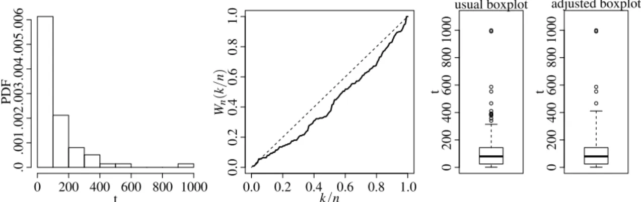
Figure 5 – Histogram, TTT plot and boxplots for the leukemia cancer data . . . 54

Figure 6 – Fitted SFs by KM method and BS, GA and IG frailty models for the leukemia cancer data. . . 55

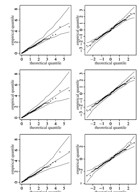
Figure 7 – QQ plot with envelope for GCS and RQ residuals for the BS, GA and IG frailty models, respectively, for leukemia cancer data . . . 56

Figure 8 – Histogram, TTT plot and boxplots for the lung cancer data . . . 57

Figure 9 – QQ plot with envelope for GCS and RQ residuals for the BS, GA and IG frailty models, respectively, with lung cancer data. . . 58

Figure 10 – Fitted SFs by KM method and BS, GA and IG frailty models for the lung cancer data. . . 59

Figure 11 – QQ plot with envelope for GCS and RQ residuals for the BS, GA and IG frailty models, respectively, with leukemia data. . . 71

Figure 12 – Generalized Cook (left) and likelihood (right) distances for leukemia data. . 71

Figure 13 – Index plots ofCifor δ under the case-weight (left), response (center) and covariate (right) perturbation schemes with leukemia data. . . 72

Figure 14 – QQ plot with envelope for GCS and RQ residuals for the BS, GA and IG frailty models, respectively, with lung cancer data. . . 75

Figure 15 – Generalized Cook (left) and likelihood (right) distances. . . 76

Figure 16 – Index plots ofCifor δ under the case-weight (left), response (center) and covariate (right) perturbation schemes with lung cancer data. . . 76

Figure 17 – Histogram, TTT plot and boxplots for the melanoma data. . . 85

Figure 18 – Index plots ofCiforα,ξξξ andbbbunder the case-weight perturbation scheme. 87 Figure 19 – Index plots ofCiforφ,ξξξ andbbbunder the response perturbation scheme. . . 87

Figure 20 – Index plots ofCiforφ,ξξξ andbbbunder the regressor perturbation scheme. . . 87

LIST OF ALGORITHMS

LIST OF TABLES

Table 1 – Conceptual analogy between material fatigue and organ growth. . . 37 Table 2 – empirical bias (with MSEs in parentheses) of the ML estimators ofδ andγ

from the BS frailty model under different censoring proportions. . . 51 Table 3 – Descriptive statistics for the observed lifetime. . . 54 Table 4 – ML estimates (with –SEs– in parentheses) and model selection measures for

the fit to leukemia data. . . 55 Table 5 – Descriptive statistics for the observed lifetime. . . 57 Table 6 – ML estimates (with estimated asymptotic standard errors –SEs– in parentheses)

and model selection measures for the fit to lung cancer data. . . 57 Table 7 – Empirical bias (with MSEs in parentheses) of the ML estimators ofγ,κ,δ

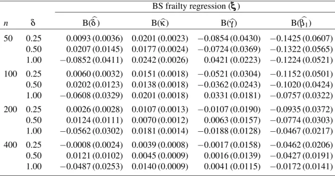
andϕ1from the BS frailty regression model. . . 64

Table 8 – Empirical mean of variance ratio. . . 65 Table 9 – ML estimates (with estimated asymptotic SEs in parentheses) and model

selection measures for the fit to leukemia data with Weibull baseline HR, and respective p-values in brackets. . . 70

Table 10 – RCs (in %) in ML estimates and their corresponding SEs for the indicated pa-rameter and dropped cases, and respective p-values in brackets with leukemia

data. . . 73 Table 11 – ML estimates (with estimated asymptotic SEs in parentheses) and model

selection measures for the fit to lung cancer data, and respectivep-values. . . 74

Table 12 – RCs (in %) in ML estimates and their corresponding SEs for the indicated parameter and dropped cases, and respectivep-values in brackets with lung

cancer data. . . 77 Table 13 – survival functionSp(t)and different cure rates for the distribution of hidden

causesN. . . 80

Table 14 – EM and EMSE of the ML estimators ofδ andγ and cure fractions for simu-lated data from the BSCrBeF model. . . 84 Table 15 – Descriptive statistics for the observed lifetime. . . 85 Table 16 – Statistics from the fitted models. . . 86 Table 17 – ML estimates of the parameters for the BSCrNBF model. . . 86 Table 18 – RCs (in %) in ML estimates and their corresponding SEs for the indicated

the BBS distribution. . . 95 Table 20 – Simulated values of biases and MSEs (within parentheses) of the ML in

comparison with those of MM estimates (δk=2.0,µk=2.0, fork=1,2), for

the BBSM distribution. . . 96 Table 21 – Probability coverages of 90% and 95% confidence intervals for the BBSM

model (µk=1.0,δk=0.5, fork=1,2). . . 98

CONTENTS

1 INTRODUCTION . . . 25 1.1 Introduction and bibliographical review . . . 25 1.2 Objectives of the thesis . . . 30 1.3 Organization of the chapters . . . 30 1.4 Products of the thesis . . . 31 2 BACKGROUND . . . 33 2.1 Introduction . . . 33 2.2 Birnbaum-Saunders distribution . . . 33 2.3 Justifying the BS distribution for medical data. . . 36 2.4 Parametrizations of the BS distribution . . . 38 2.5 Bivariate Birnbaum-Saunders distribution . . . 41 2.6 Frailty models . . . 42

2.6.1 Unconditional hazard and survival functions . . . 44

2.7 Cure rate models . . . 45 3 A BIRNBAUM-SAUNDERS FRAILTY MODEL FOR SURVIVAL

DATA . . . 47 3.1 Introduction . . . 47 3.2 Birnbaum-Saunders frailty model . . . 47

3.2.1 Model identifiability and features . . . 47

3.3 Estimation of parameters . . . 48

3.3.1 A simulation study . . . 50

3.4 Applications to real data . . . 53

3.4.1 First case study: leukemia cancer data . . . 53 3.4.2 Second case study: lung cancer data . . . 56

3.5 Concluding remarks . . . 59 4 BIRNBAUM-SAUNDERS FRAILTY REGRESSION MODELS:

DI-AGNOSTICS AND APPLICATION TO MEDICAL DATA . . . 61 4.1 Introduction . . . 61 4.2 Birnbaum-Saunders frailty regression model . . . 61

4.3.2 Local influence . . . 66 4.3.3 Residual analysis . . . 68

4.4 Applications to medical data sets. . . 68

4.4.1 Summary of the proposed methodology . . . 69 4.4.2 Application 1: leukemia data . . . 69 4.4.3 Application 2: lung cancer data. . . 72

4.5 Concluding remarks . . . 76 5 A CURE RATE FRAILTY MODEL BASED ON A

REPARAMETER-IZED BIRNBAUM-SAUNDERS DISTRIBUTION . . . 79 5.1 Introduction . . . 79 5.2 Cure rate BS frailty model . . . 79 5.3 Local influence . . . 82 5.4 Numerical evaluation . . . 83

5.4.1 Simulation study . . . 83 5.4.2 Illustrative example . . . 85

5.5 Concluding remarks . . . 88 6 ON A BIVARIATE BIRNBAUM-SAUNDERS DISTRIBUTION

PA-RAMETERIZED BY ITS MEANS . . . 89 6.1 Introduction . . . 89 6.2 Reparameterized bivariate Birnbaum-Saunders distribution . . . 89

6.2.1 Maximum likelihood estimation . . . 90 6.2.2 Modified moment estimation . . . 91

6.3 BBSM regression model . . . 92

6.3.1 Maximum likelihood estimation . . . 93

6.4 Numerical applications . . . 94

6.4.1 A simulation study . . . 94 6.4.2 BBSM simulation results . . . 95 6.4.3 Probability coverage simulation results . . . 96 6.4.4 Example 1 . . . 99 6.4.5 Example 2 . . . 100

6.5 Concluding remarks . . . 101 7 DISCUSSION, CONCLUSIONS AND FUTURE RESEARCH . . . . 103

APPENDIX A MATHEMATICAL RESULTS FOR BS FRAILTY MODEL115 A.1 Score vector . . . 115

25

CHAPTER

1

INTRODUCTION

1.1

Introduction and bibliographical review

Analysis of lifetime data plays an important role in several fields of knowledge such as economics, biology, medicine, epidemiology, engineering, demography, among others. This area has been widely studied by many researchers, with works having been published in various areas of knowledge. In this sense we can make some questions like: What distinguishes survival analysis from other areas of statistics? Why do survival data need a special statistical theory? The reason is that we are observing something that develops dynamically over time. Thus we can highlight two points related to this development. The first, survival times are usually a mixture of discrete and continuous data that lend themselves to a different type of analysis than in the traditional discrete or continuous case. The mixture is the result of censoring and has an important effect on data analysis. To put it plainly, a censored observation contains only partial information about the random variable (RV) of interest. The Kaplan-Meier estimator, proposed by Kaplan and Meier (1958), of the survival function (SF) is a major step in the development of suitable models for such kind of data. The second is because most of the evaluations are made conditionally on what is known at the time of the analysis, and this changes over time. Frequently, as the population under study is changing, we only consider the individual risk to die for those who are still alive, but this means that many standard statistical approaches cannot be applied.

information on individual values, which is often the case in demography. Furthermore, we may not know all relevant risk factors or it is impossible to measure them without great financial costs, something that is common in medical and biological studies. The neglect of covariates leads to (unobserved) heterogeneity. That is, the population consists of individuals with different risks. Another important regression model proposed in survival analysis was the accelerated failure time (AFT) model, see details in Lawless (2011). The Cox’s model and its various generalizations are mainly used in medical and biostatistical fields, while the AFT model is primarily applied in reliability theory and industrial experiments.

In this thesis we focus on frailty and cure rate frailty models as well as on a bivariate model, where all these models are based on the reparameterized Birnbaum-Saunders distribution proposed by Santos-Neto et al. (2012). In the context of frailty modeling the frailty indicates that apparently similar patients can have different risks. Thus, different patients can possess distinct frailties and then frailer patients tend to experience the event of interest earlier than those who are less frail. Therefore, frailty models have been introduced into the statistical literature in an attempt to account for the existence of heterogeneity in a population under study. In essence this concept goes back to the work of Greenwood and Yule (1920) on “accident proneness”. The RV “frailty” may be incorporated in the baseline HR additively or multiplicatively. The term frailty itself was introduced by Vaupel et al. (1979) in univariate frailty model. Several authors have studied these models, which represent a generalization of the Cox model; see Cox (1972) and Stare and O’Quigley (2004). The interested reader in frailty models is referred to Hougaard (2000), Duchateau and Janssen (2008) and Wienke (2011).

1.1. Introduction and bibliographical review 27

current status data. Chan (2014) introduced a flexible individual frailty model for clustered right-censored data, in which covariate effects can be marginally interpreted as log failure odds ratios. Zhou et al. (2015) motivated by breast cancer data proposed a covariate-adjusted proportional hazards frailty model for the analysis of clustered right-censored data. Inspired by frailty-contagion approaches used in finance and insurance, Koch and Naveau (2015) proposed a multi-site precipitation simulator that, given appropriate regional atmospheric variables, can simultaneously handle dry events and heavy rainfall periods.

In general the methods in survival analysis implicitly assume that populations are ho-mogeneous, meaning all individuals have the same risk of death, but as mentioned above, it is often important to consider the population as heterogeneous, i.e. a mixture of individuals with different hazards, for example. The frailty model is a random effects model for time-to-event data, where the frailty has a multiplicative effect on the baseline hazard function. It can be used for univariate (independent) lifetimes, i.e. to describe the influence of unobserved covariates in a proportional hazards model (heterogeneity). The variability of duration data is split into one part that depends on risk factors and is thus theoretically predictable, and one part that is initially unpredictable, even knowing all relevant information at that time. There are advantages in separating these sources of variability: heterogeneity can explain some unexpected results or give an alternative interpretation, for example crossing-over or levelling-off effects of HR. The introduction of a common random effect “the frailty” is a natural way of modeling the dependence of event times. The random effect explains the dependence in the sense that had we known the frailty, the events would have been independent. In other words, the lifetimes are conditionally independent given the frailty. This approach can be used for survival times of related individuals such as twins or family members, where independence cannot be assumed, or for recurrent events in the same individual or for times to several events for the same individual, such as onset of different diseases, relapse or death (competing risks).

et al. (2010a), Saulo et al. (2013) and Leiva et al. (2014b), Leiva et al. (2014c), Leiva et al. (2015), Leiva et al. (2015), Leiva et al. (2017). Some details about genesis and justification of the BS distribution for medical data are given in Chapter 2. Santos-Neto et al. (2012) introduced several parameterizations of the BS distribution. Specially, one of them is established in terms of the distribution mean, whereas its variance is a quadratic function of this mean. Thus, such a parameterization allows us to mimic a property of the GA frailty distribution early proposed by Vaupel et al. (1979), doing the BS frailty distribution to be a new alternative to frailty modeling. Another important area of suvival analysis is related to cure rate models (or long-term survival models). The first work in this context was proposed by Boag (1949), Berkson and Gage (1952) and refers to the mixture cure model. In this case, the population is classified into the following two subpopulations: (a) individuals who are cured with certain probability and (b) individuals exposed to risk characterized by the complementary probability, which can be estimated by using a probability distribution, for instance, exponential, Gompertz or Weibull; see Kuk and Chen (1992), Koti (2003) and Shao and Zhou (2004). A new approach for this model was presented by Yakovlev and Tsodikov (1996) and Chen et al. (1999) and refers to the non-mixture cure model, which has its structure based on the assumption that the cumulative hazard function is bounded because of the existence of cured individuals.

1.1. Introduction and bibliographical review 29

Cure rate models allow us to estimate separate covariate effects that may influence the cured fraction and the hazard of the at-risk population. If a cured fraction is not present, the analysis reduces to the standard considerations of survival data. Further details and examples of cure models and their utility are provided in Maller and Zhou (1996), Ibrahim et al. (2005) and Aalen et al. (2008). Cure models assume that the individuals experiencing the event of interest are homogeneous. However, this assumption may not be valid as unobserved heterogeneity among individuals may be present. In this sense, cure data can be analyzed utilizing statistical models that account for heterogeneity among individuals. A portion of the heterogeneity is explainable in terms of observed covariates. However, there remains a degree of heterogeneity induced by unobservable risk factors. Failing to account for this latter form of heterogeneity may lead to distorted results.

The use of bivariate distributions plays a fundamental role in many areas of knowledge, for example, in survival analysis and reliability. Here, we studied a bivariate Birnbaum-Saunders distribution parameterized by its means. The bivariate BS distribution was proposed by Kundu et al. (2010), where some other author have been extended this model as well as evaluate some properties of the model, for example Khosravi et al. (2015), Kundu et al. (2010), Kocherlakota (1986), Kundu et al. (2013), Díaz-Garcia and Leiva (2005), Vilca et al. (2014a), Vilca et al. (2014b),

1.2

Objectives of the thesis

The BS distribution has been receiving considerable attention due to its good properties. Santos-Neto et al. (2012) introduced several parameterizations for the BS distribution, where one of these reparameterizations indexes the BS distribution by its mean. Santos-Neto et al. (2014) present some mathematical properties and estimates by the maximum likelihood method, Moments and Modified moments method of the parameters from this new version of the BS distribution. According to this new BS model our gerenal objective is to study the BS frailty model. However, we can list some specific objetives

∙ to propose a new BS frailty model, which can be a good alternative to frailty modeling.

∙ to introduce a BS frailty regression model and its inference based on maximum likelihood (ML) method, and to derive influence diagnostics tools for this model. In addition, we want to apply the BS frailty regression model and its diagnostics to medical data to illustrate its potential applications and compare it with classical frailty models.

∙ to propose a cure rate Birnbaum-Saunders frailty model, where an important advantage of the proposed model is the possibility to jointly consider the heterogeneity among patients by their frailties and the presence of a cured fraction of them.

∙ to introduce a bivariate Birnbaum-Saunders distribution based on a parameterization given

by Santos-Neto et al. (2012) and Santos-Neto et al. (2014) which has the mean as one of its parameters.

1.3

Organization of the chapters

1.4. Products of the thesis 31

introduce the BS frailty model, which can be a good alternative to frailty modeling. We employ the Laplace transform to find the BS unconditional SF on the individual frailty. We use the ML method for estimating the model parameters. We investigate the asymptotic properties of the ML estimators and evaluate their performance by a Monte Carlo (MC) study. We illustrate the proposed model with uncensored and censored data. In Chapter 4, we present the BS frailty regression model and its inference based on ML methods, and to derive influence diagnostics tools for this model. In addition, we want to apply the BS frailty regression model and its diagnostics to medical data to illustrate its potential applications and compare it with classical frailty models. In Chapter 5, we propose a cure rate frailty model based on the Birnbaum-Saunders distribution as an alternative approach to modeling such data. An important advantage of the proposed cure rate frailty model is the possibility to jointly consider the heterogeneity among individuals and the presence of a cured component. We consider the ML method to estimate the model parameters and to derive influence tools. We assess local influence on the parameter estimates under different perturbation schemes. Numerical evaluation of the proposed model is considered by means of MC simulation studies and an application to a real medical data set from the medical area. In Chapter 6, we introduce a bivariate Birnbaum-Saunders distribution based on a parameterization of the Birnbaum-Saunders which has the mean as one of its parameters. We discuss the ML estimation of the model parameters and show that these estimators can be obtained by solving non-linear equations. We also discuss modified moment (MM) estimation for the unknown parameters which are easy to compute and can therefore be used as initial values to calculate the ML estimates. We derive the asymptotic distributions of these estimators and carry out a simulation study to evaluate the performance of all these estimators. The probability coverages of confidence intervals are also discussed. We then derive a regression model based on the proposed bivariate Birnbaum-Saunders distribution, which permits us to model data in their original scale. In addition, two examples are performed to illustrate the proposed methods here. Finally, we present a discussion, conclusions and future research in Chapter 7.

1.4

Products of the thesis

This thesis allowed the following products to be obtained:

∙ Leao, J., Leiva, V., Tomazella, V., Saulo H. (2017) Birnbaum-Saunders frailty regression models: Diagnostics and application to medical data.Biometrical Journal(in press);

∙ Leao, J., Leiva, V., Tomazella, V., Saulo H. (2016) A Birnbaum-Saunders frailty model for

survival data (under review forBrazilian Journal of Probability and Statistics).

∙ Saulo, H., Leao, J., Leiva, V., Tomazella, V. (2016) On a bivariate Birnbaum-Saunders distribution parameterized by its means (submitted).

33

CHAPTER

2

BACKGROUND

2.1

Introduction

In this chapter, we present some features of the BS distribution beginning with its genesis. Then, we justify the use of the BS model in medical data. We also describe briefly the parameterization used in the course of this thesis. We describe breifly the bivariate BS distribution in its original form. The interested reader in BS distribution is referred to Leiva (2016) and references therein. We present the frailty model, discuss how to obtain the unconditional HR and SF. Moreover, we discuss unified cure rate model and present some of its features; see Rodrigues et al. (2009).

2.2

Birnbaum-Saunders distribution

The Birnbaum-Saunders distribution is right-skewed (asymmetrical), continuous and unimodal. It is also known as the fatigue life distribution and has received considerable attention due to its theoretical arguments, its attractive properties and its relation with the normal distribu-tion; see the seminal paper by Birnbaum and Saunders (1969). As justification the authors used a physical argument originated from renewal theory, via idealization of the number of cycles necessary to force a fatigue crack to grow past a critical value; see, for example, Mann et al. (1974).

As a fatigue life distribution, the BS model considers a material specimen that is exposed to a sequence ofmcyclic loads,_{li,i=1,2, . . . ,m,m∈N}; for more details about this type of

load; see Saunders (2007). The loading scheme can be depicted as follows:

l1, . . . ,lm

| {z }

Cycle 1

lm+1, . . . ,l2m

| {z }

Cycle 2

. . . ljm+1, . . . ,ljm+m

| {z }

Cycle (j+1)

whereljm+i=lkm+i, for j̸=k. Birnbaum and Saunders (1969) considered that the loading is

continuous (see more details in Section 2.1), which implies that the load function, say li(·),

evaluated at the unit interval gives the amount of stress imposed on the specimen, that is,

li−1(0) =li(1) =li+1(0), i=1, . . . ,m, m∈N.

Thus, at the imposition of each load,li, the crack is extended by a random amount. Crack

extensions by cycle cannot be observed in practice and we only know the instant when the failure occurs. Having explained the physical framework of the genesis of the Birnbaum-Saunders distributions it is now necessary to make the statistical assumptions. Birnbaum and Saunders (1969) used the knowledge of certain type of materials failure due to fatigue to develop their model. The fatigue process that they used was based on the following:

(D1) A material specimen is subjected to cyclic loads or repetitive shocks, which produce a crack or wear-out in this specimen;

(D2) The failure occurs when the size of the crack in the material specimen exceeds certain level of resistance (threshold), denoted byω,

(D3) The sequence of loads imposed in the material specimen is the same from a cycle to another one;

(D4) The incremental crack extension due to a loadli, sayXi, during the jth cycle is a RV whose

distribution is governed by all the loadslj, for j<i, and by the actual crack extensions

that have preceded it in cycle alone;

(D5) The total size of the crack due to the jth cycle, sayYi, is a RV that follows a statistical

distribution of mean µ0and varianceσ₀2, and

(D6) The sizes of cracks in different cycles are mutually independent. Note that the total crack extension due to the(j+1)th cycle of load is

Yj+1=Xjm+1+Xjm+2+···+Xjm+m;j,m=0,1,2, . . . .

As mentioned by Mann et al. (1974), assumption (D4) is rather restrictive and may not be valid for certain applications. This assumption ensures that, regardless of the dependence among the successive random extensions due to the loads in a particular cycle, the total random crack extensions are independent from cycle to cycle. The plausibility of this assumption in aeronautical fatigue studies is briefly stated by Birnbaum and Saunders (1969).

The BS model looks for the distribution of the smallestn, sayn*, such that the sum

Sn=

n

∑

2.2. Birnbaum-Saunders distribution 35

ofnpositive RV exceeds the given thresholdω, that is,

n*=inf_{n_∈N;_Sn=

n

∑

Yj>ω}.

In the simplest case, the BS distribution is derived by supposing that theYj are

indepen-dent and iindepen-dentically distributed RV, then applying the central limit theorem and then by regarding

n*as a continuous RVT.

Specifically, based on the central limit theorem, Equation (2.1), and the assumptions (D5) and (D6) made by Birnbaum and Saunders (1969), asn_→∞, it is possible to establish that

Sn∼· N(nµ0,nσ02). (2.2)

LetN be the number of required cycles until the failure. Given thatYj>0 for all j≥1,

the damage is irreversible and so by complementarity, we have_{N >n_{} ≡ {}Sn≤ω}and we

have_{N_≤n_{} ≡ {}Sn>ω}. Then, from assumption (D5) and and (2.1), we have that E(Sn) =nµ0

and Var(Sn) =nσ₀2. Therefore, by standardizing (2.2), we get

P(N_≤n) _≈ P

Sn−nµ0

σ0√n >

ω₋nµ0

σ0√n

= P

Sn−nµ0

σ0√n ≤

nµ0−ω

σ0√n

= Φ

nµ0−ω

σ0√n

= Φ

√_{ω µ}

0

σ0

n

ω/µ0−

ω/µ0

n

. (2.3)

Birnbaum and Saunders (1969) used Equation (2.3) to define a continuous life distribu-tion, idealizing the discrete variateN through a continuous variateT and the discrete argumentn

by means of the continuoust, that is, the number of cycles until the failure,N, is replaced by the

total time until that the failure occurs,T, andnth cycle by the timet. Thus, taking

α = _√σ0

ω µ0 andβ =

ω µ0,

and

at(α,β) =at =

1

α

 

s

t

β −

r

β

t



, (2.4)

we obtain that

which is the cumulative distribution function (CDF) of the BS distribution with shape and scale parameters,α andβ, respectively. This means that we are admitting as definition that a

random variableT follows the BS distribution with shape and scale parametersα>0 andβ >0,

respectively, if it can be written as

T =β

"

α

2Z+

r_α

2Z

2 +1

#

, (2.5)

whereZ is a random variable following the standard normal distribution, such that

Z= 1

α

 

s

T

β −

r

β

T



_∼N(0,1) (2.6)

The derivation of Birnbaum and Saunders (1969) supposes some aspects about the growth of a crack that are questionable. Desmond (1985) gave a more general derivation for this distribution as well as derived the BS distribution using a biological model discussed by Cramér (1947). In the next subsection we present some of these arguments presented in Desmond (1985) that justify the use of the BS model in medical data.

2.3

Justifying the BS distribution for medical data

Assuming a BS distribution to model medical data based on an empirical fitting can be a reasonable argument. However, the argument may be strengthened if we justify why the BS distribution might be suitable for such a modeling. Cramér’s biological model, linked to the proportionate-effect model, allows us to justify the BS distribution within a medical setting.

Consider a RV related to the size of a human organ. The size may be considered as the joint effect of a large number of independent causes. The causes act sequentially through the time of organ growth. If the effects of causes are summed and assumed as RVs, then the sum follows an asymptotic normal distribution due to the central limit theorem. However, the causes do not seem to jointly operate by simple addition. It seems more natural to assume that each cause provides an impulse. Thus, the effect depends on both the impulse strength and the organ size attained at the instant when the impulse is working. Specifically, letY1, . . . ,Ynbe independent

RVs corresponding to the magnitude ofnimpulses, which act sequentially according to their

sub-indices. In addition, let Xj be the size of an organ, which is produced by the impulses.

Assume thatXj+1increases proportionally to the(j+1)th impulseYj+1and to some function

g(Xj)of the organ size as

Xj+1=Xj+Yj+1g(Xj), j=0,1, . . . . (2.7)

Therefore,Xj+1is the accumulated size of the organ after application of the impulseYj+1.

2.3. Justifying the BS distribution for medical data 37

can be obtained wheng(X) =1. Relationship defined in (2.7) has been proposed in biological and fatigue contexts; see Desmond (1985). The BS distribution was built to model fatigue life of material specimens subject to cyclic stress. It provokes a damage that is accumulated over time by a sum of numerous small damages. When the damage exceeds a rupture threshold of the specimen, it fails; see Birnbaum and Saunders (1969). Table 1 provides a conceptual analogy between fatigue and medical settings.

Table 1 – Conceptual analogy between material fatigue and organ growth.

❳ ❳

❳ ❳

❳ ❳

❳ ❳

❳ ❳

❳ ❳

Process

Concept

Specimen Cause Threshold Effect RV Fatigue Material Damage Rupture Failure Fatigue life Growth Organ Impulse To die Death Time of death

We put Frost & Dugdale’s model, often used in engineering; see Frost and Dugdale (1958), in a medical setting by

da

dn=

S3a

c =c1f(∆K), (2.8)

whereais the organ size,nthe number of impulses,Sthe strength applied in each impulse,ca

constant,∆K the range of a strength intensity factor, f(_·)an empirically determined function

andc1an experimental constant. One can relate∆Kin (2.8) to the organ sizeaby means of

∆K=b∆Sa1/2, (2.9)

whereb is a geometrically related parameter and ∆S the strength amplitude applied in each

impulse. Based on (2.8) and (2.9), and approximating f(_·)by f(b∆Sa1/2)_≈c0+c2g(a), with

g(_·)being a function of the organ size, we have

da

dn ≈c0+c3g(a), (2.10)

where c3 contains constants c1,c2, and c0 is the initial organ size, with c0, a and c3 being

considered as RVs to make it closer to reality.

Note the similarity between differential-equation model (2.10) and proportionate-effect model (2.7). Retake (2.7), apply the central limit theorem and consider the increment ∆X_j=

Xj+1−Xj in the(j+1)th impulse gives a small contribution to the organ growth. Then,

summa-tion can be changed by integrasumma-tion. Thus, we get

n

∑

Yj=

n

∑

∆X_j

g(Xj) ≈

Z Xn

X₀

dx

g(x) =log(g(Xn))−log(g(X0)),

follows approximately a normal distribution, whereX₀is the initial organ size andXnits final

To obtain the BS distribution in this setting, suppose that the mean ofXj isη and its

varianceρ2. This generalizes Assumption 2 of Birnbaum and Saunders (1969) and conducts to

I(X(t)) =

Z X(t)

X0

1

g(x)dx∼N(tη,tρ

2_{), (2.11)}

whereX(t)is the organ size at timet. Assume now thatXc>X0is a critical organ size at which

death occurs. Then,T =inf_{t:X(t)>Xc}is the time of death. Therefore, from (2.11) and using

the equivalent events_{T _≤t_}and_{X(t)>Xc}, it follows that the CDF ofT is

FT(t) =Φ((tη−I(Xc))/

√

tρ), (2.12)

whereΦis the CDF of the standard normal distribution. From (2.12), note that choice of the

functiong(X)in the model given in (2.7) determines the dependence of the organ size on the

previous size. A power function forg(X)could be a reasonable choice depending on the type of organ. Suppose thatg(X) =Xδ, whereδ could be a parameter related to the type of organ. In this case, from (2.11), note thatX(t)1−δ _∼N(X₀1−δ+ [1₋δ]tη,[1₋δ]2tρ2)and then the CDF ofT is

FT(t) =

        

Φ

Xc1−δ−X01−δ+[δ−1]tη [δ−1]√tρ

, ifδ >1;

Φ

X₀1−δ−X_c1−δ+[1−δ]tη

[1−δ]√tρ

, ifδ <1.

(2.13)

Therefore, the LN distribution is obtained from (2.13) by lettingδ _→1, whereas the BS distribu-tion results forδ =0. However, although the caseδ =1 corresponds to the proportionate-effect model, the life distribution itself is of the BS type and not of LN type, see Desmond (1985).

2.4

Parametrizations of the BS distribution

Santos-Neto et al. (2012) proposed several parameterizations of the BS distribution, which allow diverse features of data modeling to be considered. One of such parameterizations is indexed by the parametersµ =β(1+α2/2)andδ =2/α2, whereα >0 andβ >0 are the original BS parameters; see Birnbaum and Saunders (1969), µ >0 is a scale parameter and the mean of the distribution, whereasδ >0 is a shape and precision parameter. The notation

U _∼BS(µ,δ) is used when the RVU follows such a distribution. This parameterization of

the BS distribution permits us to mimic a property of the GA distribution, which was the first distribution used in a frailty model Vaupel et al. (1979) as follows. The mean and variance of

U _∼BS(µ,δ)are E[U] =µ and Var[U] =µ2/φ, respectively, where φ = (δ+1)2/(2δ+5).

2.4. Parametrizations of the BS distribution 39

IfU _∼BS(µ,δ), then its probability density function (PDF) is

fU(u;µ,δ) =

exp(δ/2)√δ+1 4u32√_{π µ}

u+ δ µ

δ+1

exp

−δ₄

u(δ+1)

δ µ + δ µ

u(δ+1)

, u>0.

(2.14) It is possible to show that kU _∼BS(kµ,δ), with k>0, and 1/U _∼BS(µ*,δ), where µ*= (δ+1)/(δ µ), that is, the BS distribution, in its original and reparameterized forms, is closed under scaling and reciprocation. From (2.14), the SF and HR ofU are, respectively,

SU(u;µ,δ) = 1

2Φ(u+δ(u−µ)/(2

p

u(1+δ)µ)), u>0,

hU(u;µ,δ) =

exp(₋(₋δ µ+δu+u)2/(4(δ+1)µu))(δ µ+δu+u)

(π µ(δ+1))122_µ12_u32Φ((u+δ(u₋µ))/(2pu(1+δ)µ)), u>0,

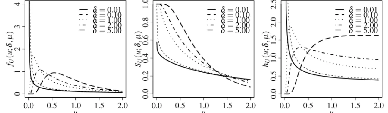
whereΦis the CDF of the N(0, 1) distribution. Figure 1 displays some shapes for the PDF, SF

and HR ofU _∼BS(µ =1,δ). Note that a unimodal behavior is detected for the PDF, as well

as different degrees of asymmetry and kurtosis, whereas the HR has increasing and decreasing shapes, such as the GA distribution, but also an inverse bathtub shape.

fU ( u ; δ , µ ) u 0 1 2 3 4

0.0 0.5 1.0 1.5 2.0

δ=0.01

δ=0.10

δ=1.00

δ=2.00

δ=5.00

SU ( u ; δ , µ ) u 0 .0 0.0 0 .2 0 .4 0.5 0 .6 0 .8 1 .0

1.0 1.5 2.0

δ=0.01

δ=0.10

δ=1.00

δ=2.00

δ=5.00

hU ( u ; δ , µ ) u 0 .0 0.0 0 .5 0.5 1 .0 1.0 1 .5 1.5 2 .0 2.0 2 .5

δ=0.01

δ=0.10

δ=1.00

δ=2.00

δ=5.00

Figure 1 – Plots of PDF, SF and HR of the BS distribution forµ=1 and different values ofδ.

The use of the BS distribution has the following appealing advantages:

∙ Based on its genesis, it is possible to make an analogy in the modeling of medical data;

see, for example, Desmond (1985).

∙ Its parameterization based on the mean (µ), such as in (2.14), allows us to analyze data in their original scale, avoiding, for instance, problems of interpretation in models which employ a logarithmic transformation of the data; see Leiva et al. (2014a) and Santos-Neto et al. (2014).

∙ In the context of frailty models, it can be very competitive in terms of fitting.

∙ It belongs to the class of log-symmetric distributions, such as the case of the generalized BS, LN, log-logistic, log-Laplace, log-Student-t, log-power-exponential, log-slash and

reciprocal or as ordinary symmetry of the distribution of the logged RV; see Jones (2008). One can obtain the BS, LN and logistic frailty models as particular cases of log-symmetric frailty models. However, besides the BS frailty model which is proposed in this thesis, the only other popular log-symmetric frailty model that belongs to this class is the LN one. But unlike the BS frailty model, the LN model does not have an explicit Laplace transform; see Wienke (2011). This explicit form is useful to obtain the PDF and the unconditional SF and HR.

∙ It is flexible in terms of bimodality when the logarithm of a BS RV is taken into account.

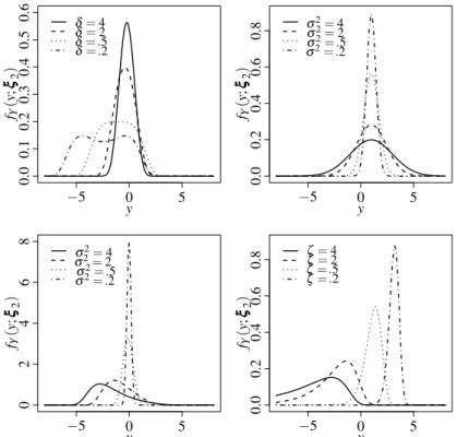
Note that:

(i) If U _∼ BS(1,δ), Y = log(U) _∼ log-BS(p2/δ,log(δ/(δ +1))); see Rieck and

Nedelman (1991);

(ii) IfU_∼LN(1,σ2),Y =log(U)_∼N(1,σ2); see Crow and Shimizu (1988);

(iii) IfU_∼IG(1,σ2),Y =log(U)_∼log-IG(σ2,0); see Kotz et al. (2010b);

(iv) IfU_∼GA(1/ζ,1/ζ),Y =log(U)_∼log-GA(1/ζ,1/ζ); see Johnson et al. (1995).

Some properties of the log-BS distribution are as follows. IfY_∼log-BS(p2/δ,log(δ µ/(δ+

1))), then: (a)U=exp(Y)_∼BS(µ,δ); (b) E(Y) =log(δ µ/(δ+1)); (c) there is no closed form for the variance ofY, but based upon an asymptotic approximation for the log-BS

moment generating function, it follows that, as δ _→∞, Var(Y) =2/δ₋1/δ2, whereas that, in contrast, asδ _→0, Var(Y) =4(log2(2/√δ) +2₋2 log(2/√δ)); and (d) the dis-tribution ofY is symmetric aroundµ, unimodal forδ _≥0.5 and bimodal forδ <0.5; see

Rieck and Nedelman (1991) and Leiva (2016). Figure 2 shows some shapes for the PDF ofY =log(U)in each aforementioned distribution. Note that the bimodality property is

2.5. Bivariate Birnbaum-Saunders distribution 41 fY ( y ; ξξξ2 ) y

−5 0 5

0 .0 0 .1 0 .2 0 .3 0 .4 0 .5 0 .6

δ=4

δ=2

δ=.5

δ=.2

fY ( y ; ξξξ2 ) y

−5 0 5

0 .0 0 .2 0 .4 0 .6 0

.8 σ_σ22=₌4₂

σ2_=.5

σ2_=.2

fY ( y ; ξξξ2 ) y −5 0 0 2 4 5 6 8

σ2₌₄

σ2₌₂

σ2_=.5

σ2_=.2

fY ( y ; ξξξ2 ) y

−5 0 5

0 .0 0 .2 0 .4 0 .6 0

.8 ζζ==42

ζ=.5

ζ=.2

Figure 2 – PDF plots of the log-BS(p2/δ,log(δ/(δ+1))), N(1,σ2), log-IG(σ2,0)and log-GA(1/ζ,1/ζ) distri-butions.

2.5

Bivariate Birnbaum-Saunders distribution

Kundu et al. (2010) introduced the bivariate Birnbaum-Saunders (BBS) distribution, where the authors discussed maximum likelihood estimation and modified moment estimation of the model parameters. Recently, Khosravi et al. (2015) observed that the bivariate BS proposed in Kundu et al. (2010) can be written as the weighted mixture of bivariate inverse Gaussian distribution and its reciprocals; see Kocherlakota (1986). They also introduced a mixture of two bivariate BS distributions and discussed its various properties. Kundu et al. (2013) extended to the multivariate case, the generalized BS distribution introduced by Díaz-Garcia and Leiva (2005). Other bivariate and multivariate distributions related to the BS model can be found in Vilca et al. (2014a), Vilca et al. (2014b), Kundu et al. (2015), Kundu (2015) and Jamalizadeh and Kundu (2015).

If the random vector TTT = (T1,T2)⊤ is BBS distributed with parameter vectors ααα = (α1,α2)⊤ andβββ = (β1,β2)⊤, and correlation coefficientρ, denoted byTTT ∼BBS(ααα,βββ,ρ), then

FBBS(ttt;ααα,βββ,ρ) =Φ2   1 α1   r t1

β1− s

β1

t1

 , 1

α2  

r

t2

β2− s

β2

t2

 ;ρ,gc



, ttt>000, (2.15)

fBBS(ttt;ααα,βββ,ρ) = φ2

  1

α1  rt1

β1− s

β1

t1

 , 1

α2  rt2

β2− s

β2

t2

 ;ρ



 (2.16)

×₂1_α

1 ( β1 t1 1 2 + β1 t1 3

2) ₁

2α2 ( β2 t2 1 2 + β2 t2 3 2)

, ttt>000,

whereαk>0 andβk>0 fork=1,2,−1<ρ<1, andφ2(·,·;ρ)is a normal joint PDF given by

φ2(u,v;ρ) = 1

2πp1₋ρ2exp

₁ (1₋ρ2)(u

2_+v2

−2ρuv)

.

Kundu et al. (2010) present some properties of the BBS distribution, for example

Proposition 1IfTTT = (T1,T2)⊤∼BBS(ααα,βββ,ρ), then

a)TTT−1= (T₁−1,T₂−1)⊤_∼BBS(α1,1/β1,α2,1/β2,ρ);

b)TTT−₁1= (T₁−1,T₂)⊤_∼BBS(α1,1/β1,α2,β2,−ρ);

c)TTT−₂1= (T1,T₂−1)⊤_∼BBS(α1,β1,α2,1/β2,₋ρ);

Proposition 2IfTTT = (T1,T2)⊤∼BBS(ααα,βββ,ρ), then

a) The conditional PDF ofT1, givenT2=t2is given by

f_T1|T2=t2(t1) = 1

α1β1p2π(1−ρ2) "

β1

t1

1/2 +

β1

t1

3/2#

× exp     − 1 2(1₋ρ2)

  1

α1  rt1

β1− s

β1

t1

 ₋ ρ

α2  rt2

β2− s β2 t2    

2_   

b) The conditional CDF ofT1, givenT2=t2is given by

P[T_1≤t_1|T₂=t₂] = Φ

       1 α1 q t1

β1−

q

β1 t1

−αρ2

q

t2

β2−

q

β2 t2

p

1₋ρ2

      

2.6

Frailty models

2.6. Frailty models 43

on an unobservable RV U, which acts multiplicatively on the baseline HR. Therefore, the

conditional HR of the lifetimeT, givenU =uifor the patientiat timet, is

h_T|U=ui(t;ξξξ₁,ξξξ₂) =uih0(t;ξξξ1), i=1, . . . ,n, t>0, (2.17)

whereui is the frailty of the patienti and h0 is a baseline HR, that is, we consider the case

with a proportional HR. In (2.17), note that ξξξ₁ and ξξξ₂ are vectors of the model parameters related to the lifetime and frailty distributions, respectively, of the patienti. In addition, observe

that (2.17) is known as the Clayton model; see Clayton (1991). From (2.17), a patient i is

called “standard” if his/her frailty isui=1; “twice as likely to die” if his/her frailty isui=2,

at any particular time and in relation to the standard patient; and “one-half as likely to die” if his/her frailty isui=1/2; see Vaupel et al. (1979). The corresponding conditional SF ofT is S_T|U=ui(t;ξξξ₁,ξξξ₂) = (S0(t;ξξξ1))ui, fori=1, . . . ,nandt >0, which represents the probability of

the patientito be alive at timet given the random effectUi=ui.

If values of covariates in the model given in (2.17) are introduced similarly to the Cox model, we have

h_T|U=ui(t;xxx,ξξξ) =uih0(t;ξξξ1)exp(xxxi⊤ϕϕϕ), i=1, . . . ,n, t >0, (2.18)

wherexxx⊤_i = (1,x1i, . . . ,xpi)is a vector containing the values of pcovariates for the patienti,ϕϕϕ=

(ϕ0,ϕ1, . . . ,ϕp)⊤is the vector of regression coefficients to be estimated, andξξξ= (ξξξ⊤1,ξξξ⊤2,ϕϕϕ⊤)⊤.

Therefore, the frailty model given in (2.18) is a generalization of the proportional hazard model, which is obtained when the frailty distribution degenerates atU =1 for all patients. The

corresponding conditional SF can be obtained from (2.18) as

S_T|U=ui(t;xxx,ξξξ) =exp(₋uiH0(t;ξξξ1)exp(xxx⊤ϕϕϕ)), i=1, . . . ,n, t>0, (2.19)

whereH0(t;ξξξ1) =R0th0(s;ξξξ1)dsis the baseline cumulative hazard rate (CHR).

Suppose that the lifetime is not completely observed and may be subject to right censoring. Letvidenote the censoring time,yithe time to event of interest anduithe frailty for the patienti,

respectively. We observeti=min{yi,vi}, that is, if the censoring indicatorςi=1,ti=yiis the

lifetime of the patienti; otherwise, ifςi=0,ti=viis the right censoring time of the patienti; for i=1, . . . ,n. Then, from (2.18) and (2.19), the corresponding likelihood function is

L(ξξξ;ttt,ςςς,xxx,uuu) =L(ξξξ) =

n

∏

uih0(t;ξξξ1)exp(xxx⊤ϕϕϕ)

ςi

exp₋uiH0(t;ξξξ1)exp(xxx⊤ϕϕϕ)

, (2.20)

whereξξξ is defined in (2.18),ttt= (t1, . . . ,tn)⊤ are the lifetimes of the patients,ςςς = (ς1, . . . ,ςn)⊤

is the vector of their censoring indicators, anduuu= (u1, . . . ,un)⊤ is the vector of their frailties.

Now, conditional on the unobserved frailties uuu, the likelihood function given in (2.20) forms

the basis for the parameter estimation. The frailtiesuuumust be integrated out (in closed form or

function (not depending on unobserved quantities) of the type

L(ξξξ;ttt,ςςς,xxx) =L(ξξξ) =

n

∏

(hT(ti;xxx,ξξξ))ςiST(ti;xxx,ξξξ), (2.21)

wherehT andST are the unconditional HR and SF, respectively, defined next.

2.6.1

Unconditional hazard and survival functions

The unconditional (population) SF of T can be obtained by integrating S_T|U=ui(t;xxx)

given in (2.19) on the frailtyU. It may be viewed as the (unconditional) SF of patients randomly

drawn from the population under study; see Klein and Moeschberger (2003), Aalen et al. (2008) and Wienke (2011). Unconditional HF and SF can be obtained with the Laplace transform; see Hougaard (1984). Then, when seeking distributions for the frailty RVU, it is natural to use

frailty distributions with an explicit Laplace transform, because it facilitates the use of standard ML methods for parameter estimation. To get the unconditional SF, we need to integrate out the frailty component as

ST(t;xxx,ξξξ) =

Z ∞

0 ST|U=u(t;xxx,ξξξ)fU(u;ξξξ2)du, (2.22)

whereξξξ is defined in (2.18), S_T|U=u(t;xxx,ξξξ) =exp(₋uH0(t;ξξξ1)exp(xxx⊤ϕϕϕ))is the conditional

SF as given in (2.19) and fU is the corresponding frailty PDF. The Laplace transform of real

argumentsof a function f is

Q(s) =

Z ∞

0 exp(−sx)f(x)dx. (2.23)

Let f = fU be the frailty PDF ands=H0(t;ξξξ1)exp(xxx⊤ϕϕϕ). Then, according to (2.23), we obtain

the Laplace transform of the unconditional SF ofT as

ST(t;xxx,ξξξ) =

Z ∞

0 exp(−uH0(t;ξξξ1)exp(xxx

⊤_ϕϕϕ))f

U(u;ξξξ2)du=Q(H0(t;ξξξ1)exp(xxx⊤ϕϕϕ)). (2.24)

Note that (2.24) conducts to the same form as the unconditional SF given in (2.22); see Vaupel et al. (1979) and Wienke (2011). The frailty RVsUiare usually assumed to be independent with

2.7. Cure rate models 45

2.7

Cure rate models

The unified long-term survival model has its formulation based on a biological context as in Yakovlev and Tsodikov (1996) and Chen et al. (1999); further details can be seen in Rodrigues et al. (2009). For a subject in the population, we represent byNthe number of competing causes

related to the occurrence of an event of interest. Given N=nthe promotion time for the jth

competing cause is denoted by Zj, j=1, . . . ,n. We assume that, conditional on N, the Zj’s

are independent and identically distributed (IID). We suppose also that N is independent of

(Z1, . . . ,Zn). The observable time to event is defined asT =min{Z1,Z2, . . . ,ZN}forN≥1, and T =∞if N=0, which leads to a cure fraction p0. According to Rodrigues et al. (2009), the

long-term survival function of the RVT is given by

Sp(t) =P(T ≥t) =P(N=0) +

∞

∑

P(Z1>t, . . . ,ZN>t|N=n)P(N =n)

= ∞

∑

P(N=n)[S*_T(t)]n=A_N[S*

T(t)], (2.25)

whereS*_T(_·)denotes the common survival function of the unobserved lifetimes andA_N[·]is the

probability generating function of the RVN, which converges whenu=S*_T(t)_∈[0,1]. Thus,

various results can be obtained for each choice of the generating function of the distribution ofN

andS*_T(t). More details about this model can be found in Rodrigues et al. (2009).

In this work, we assume that the unobserved latent variableN has a negative binomial

distribution Piegorsch (1990), Saha and Paul (2005) with probability mass function given by

P(N=n) =Γ(n+φ−

1₎

n!Γ(φ−1₎

φ θ

1+φ θ

n

(1+φ θ)−1/φ, (2.26)

withn=0,1, . . .,θ >0,φ _{≥ −}1 and 1+φ θ >0, so thatE_{(N) =θ} and Var_{(N) =θ+φ θ}2.

As discussed by Tournoud and Ecochard (2007), the parameters of the negative binomial distribution have biological interpretations. The mean of the number of competing causes is represented byθ, whereasφ is the dispersion parameter. The variance of the number of initiated cells is flexible: there is under-dispersion in the Poisson model when₋1/θ <φ <0, whereas forφ >0 over-dispersion is present. The negative binomial model comprises some well-known models when the parameterφ is fixed. For instance, ifφ _→0 the probability function of the Poisson distribution is obtained, when φ =₋1 the Bernoulli distribution and if φ =1 the geometric distribution. Therefore, considering the number of competing causes to be negative binomial distributed andS*_T(_·)a proper SF, we have that the long-term SF of the RVT is given

by

Sp(t) ={1+φ θ(1−S*T(t))}−1/φ, (2.27)

where p₀=limt→∞Sp(t) = (1+φ θ)−1/φ >0, p0represents the proportion of cured or immune

SF which is given by

fp(t) = fT*(t)

_dA (u)

du |u=S*T(t)

, (2.28)

and the long-term hazard function is defined as

hp(t) = fp(t)

Sp(t)

= f_T*(t) dA_(u)

du |u=S*T(t)

Sp(t)

. (2.29)

From (2.28) and (2.29) the corresponding PDF and HR become

fp(t) =θfT*(t){1+φ θ[1−S*T(t)]}−1/φ−1, (2.30)

and

hp(t) =θfT*(t){1+φ θ[1−S*T(t)]}−1. (2.31)

47

CHAPTER

3

A BIRNBAUM-SAUNDERS FRAILTY MODEL

FOR SURVIVAL DATA

3.1

Introduction

In this chapter, we introduce the BS frailty model, discuss aspects of model identifiability, estimate its parameters, introduce two residuals, conduct a simulation study to evaluate the behavior of the parameter estimators and illustrate the potentiality of the proposed model with two real-world data sets. Here, we consider BS frailty model without observed covariates, but they will be explicitly considered in the next chapter.

3.2

Birnbaum-Saunders frailty model

In this section, we discuss some model identifiability issues and how to estimate the model parameters via the ML method and to infer about these parameters.

3.2.1

Model identifiability and features

In univariate frailty models, an important aspect is its identifiability. In the context of proportional hazard models, when working with frailty, it is necessary that the random effect distribution has finite mean for the model to be identifiable; see Elbers and Ridder (1982). Thus, in order to keep the identifiability of the model, it is convenient to take the distribution with mean equal to one. We assume that the frailtyU has a BS distribution with parametersµ =1 andδ, where E[U] =1 and Var[U] = (2δ+5)/(δ+1)2. The variance quantifies the amount of heterogeneity among patients.

From (2.22), the Laplace transform for the BS distribution with parametersµ =1 andδ

Q(s) =

expδ

2 1−

√

δ+4s+1/√δ+1 √δ+4s+1+√δ+1

2√δ+4s+1 . (3.1)

From (2.22) and evaluating (3.1) ats=H0(t), we obtain the unconditional SF under the

BS frailty as

ST(t) =

exp(δ₂(1₋pδ+4H0(t) +1/√δ+1))(pδ+4H0(t) +1+√δ+1)

2pδ+4H0(t) +1

. (3.2)

Then, from (3.1), the corresponding unconditional HR is given by

hT(t) =h0(t)

δ(δ+√δ+1pδ+4H0(t) +1+4H0(t) +3) +2 (δ+4H0(t) +1)(δ+√δ+1pδ+4H0(t) +1+1)

!

. (3.3)

We assume that the baseline HRh0(t) is specified up to a few unknown parameters,

which are related to a distribution assumed for the baseline hazard. For example, we can suppose an exponential, LN or Weibull distribution. However, assuming a parametric distribution is not always desirable, because such a assumption is often difficult to verify. Note that the exponential distribution has been extensively used to model the baseline HR due to its simplicity or when the HR must be constant for each patient; see Lawless (2011). Therefore, we use the exponential distribution as baseline hazard, which hash0(t) =γ andH0(t) =γt, fort>0. Thus, from (3.3),

the unconditional HR under BS frailty reduces to

hT(t) =

γ(δ(δ+√δ+1pδ+4γt+1+4γt+3) +2)

(δ+4γt+1)(δ+√δ+1pδ+4γt+1+1) , (3.4)

whereγ is the average HR of each patient. From (3.2), the unconditional SF under BS frailty is

ST(t) =

exp1₂δ1₋pδ+4γt+1/√δ+1√δ+1+pδ+4γt+1

2pδ+4γt+1 . (3.5)

Note that (3.2) and (3.3) can be easily applied to different baselines other than the exponential one. In fact, in Section 3.4 we also consider a Weibull baseline.

3.3

Estimation of parameters

3.3. Estimation of parameters 49

the corresponding likelihood function under uninformative censoring can be expressed as

L(ξξξ) =

n

∏

 γ(δ

δ+√δ+1pδ+4γti+1+4γti+3

+2) (δ+4γti+1)δ+√δ+1pδ+4γti+1+1

 

ςi

×

  

exp(1₂δ(1₋

√_δ

+4γti+1

√

δ+1 )(

√

δ+1+pδ+4γti+1)

2pδ+4γti+1

 

. (3.6)

Therefore, the log-likelihood function for the BS frailty model obtained from (3.6) is given by

ℓ(ξξξ) = nδ

2 −

δ

2√δ+1

n

∑

p

δ+4γti+1− n

∑

ςilog(δ+4γti+1)

− n

∑

log(2pδ+4γti+1) + n

∑

log(pδ+1+pδ+4γti+1)

+

n

∑

ςilog(γ(δ(δ+

p

(δ+1)(δ+4γti+1) +4γti+3) +2))

− n

∑

ςilog(δ+

p

(δ+1)(δ+4γti+1) +1). (3.7)

Then, the first derivatives of the log-likelihood function with respect to the two parameters can be obtained; see Appendix A. The ML equations forδ andγ must be solved with an iterative method for non-linear optimization problems. Specifically, the ML estimates of the BS frailty model parameters can be obtained by using the Broyden-Fletcher-Goldfarb-Shanno (BFGS) quasi-Newton non-linear optimization algorithm with numeric derivatives; see Nocedal and Wright (2006) and Lange (2010). The BFGS method is implemented in theRsoftware by the

functionsoptimandoptimx; see <www.R-project.org> and R Core Team (2016).

Standard regularity conditions; see for example Cox and Hinkley (1979), Serfling (1980), Lehmann and Casella (2006), Migon et al. (2014), are fulfilled for the proposed model, when-ever the parameters are within the parameter space. It is well known the ML estimators are asymptotically normally distributed. Thus, for the BS frailty model, we have

b

ξξξ _→D N2(ξξξ,ΣΣΣξ),

whereΣΣΣ_ξ is the asymptotic variance-covariance matrix of ξξξb and _→D denotes convergence in distribution. Therefore, an approximate 100_×(1₋ϖ)% confidence interval (CI) forξξξ is

R=_{ξξξ _∈R2:_|ξξξb_−ξξξ|⊤ΣbΣΣ_ξξξ−1_|ξξξb₋ξξξ_{| ≤}χ_2;12 _−ϖ}, 0<ϖ<1, (3.8)