time-dependent structure based on the inverse
gaussian distribution
PROGRAMA INTERINSTITUCIONAL DE PÓS-GRADUAÇÃO EM ESTATÍSTICA UFSCar-USP
LIA HANNA MARTINS MORITA
DEGRADATION MODELING FOR RELIABILITY ANALYSIS WITH TIME-DEPENDENT STRUCTURE BASED ON THE INVERSE
GAUSSIAN DISTRIBUTION
Thesis submitted to the Departamento de Estatística – Des/ UFSCar and to the Instituto de Ciências Matemáticas e de Computação – ICMC-USP, in partial fulfillment for the PhD degree in Statistics - Interinstitutional Program of Pos-Graduationin Statistics UFSCar-USP.
Advisor: Profa. Dra. Vera Lucia Damasceno Tomazella
PROGRAMA INTERINSTITUCIONAL DE PÓS-GRADUAÇÃO EM ESTATÍSTICA UFSCar-USP
LIA HANNA MARTINS MORITA
MODELAGEM DE DEGRADAÇÃO PARA ANÁLISE DE CONFIABILIDADE COM ESTRUTURA DEPENDENTE DO TEMPO BASEADA NA
DISTRIBUIÇÃO GAUSSIANA INVERSA
Tese apresentada ao Departamento de Estatística – Des/UFSCar e ao Instituto de Ciências Matemáticas e de Computação – ICMC-USP, como parte dos requisitos para obtenção do título de Doutor em Estatística - Programa Interinstitucional de Pós-Graduação em Estatística UFSCar-USP.
Orientadora: Profa. Dra. Vera Lucia Damasceno Tomazella
MORITA, L. H. M.. Modelagem de degradação para análise de confiabilidade com estrutura dependente do tempo baseada na distribuição gaussiana inversa. 2017. 131 p. Tese (Estatística - Programa Interinstitucional de Pós-Graduação em Estatística) - Departamento de Estatística - DEs-UFSCar e Instituto de Ciências Matemáticas e de Computação - ICMC-USP, São Carlos - SP.
As técnicas convencionais de análise de confiabilidade são voltadas para a ocorrência de falhas ao longo do tempo. Contudo, em determinadas situações nas quais a ocorrência de falhas é pequena ou quase nula, a estimação das quantidades que descrevem os tempos de falha fica comprometida. Neste contexto foram desenvolvidos os modelos de degradação, que possuem como dado experimental não a falha, mas sim alguma característica mensurável a ela atrelada. A análise de degradação pode fornecer informações sobre a distribuição de vida dos componentes sem realmente observar falhas. Assim, nesta tese nós propusemos diferentes metodologias para dados de degradação baseados na distribuição gaussiana inversa. Inicialmente, nós introduzimos o modelo de taxa de deterioração gaussiana inversa para dados de degradação e um estudo de suas propriedades assintóticas com dados simulados. Em seguida, nós apresentamos um modelo de processo gaussiano inverso com fragilidade considerando que a fragilidade é uma boa ferramenta para explorar a influência de covariáveis não observadas, e um estudo comparativo com o processo gaussiano inverso usual baseado em dados simulados foi realizado. Também mostramos um modelo de mistura de processos gaussianos inversos em testes de burn-in, onde o principal interesse é determinar o tempo de burn-in e o ponto de corte ótimo para separar os itens bons dos itens ruins em uma linha de produção, e foi realizado um estudo de má especificação com os processos de Wiener e gamma. Por fim, nós consideramos um modelo mais flexível com um conjunto de pontos de corte, em que as probabilidades de má classificação são estimadas através do método exato com distribuição gaussiana inversa bivariada ou em um método aproximado baseado na teoria de cópulas. A aplicação da metodologia foi realizada com três conjuntos de dados reais de degradação de componentes de LASER, rodas de locomotivas e trincas em metais.
MORITA, L. H. M.. Degradation modeling for reliability analysis with time-dependent structure based on the inverse gaussian distribution. 2017. 131 p. Thesis (Statistics - Programa Interinstitucional de Pós-Graduação em Estatística) - Departamento de Estatística - DEs-UFSCar and Instituto de Ciências Matemáticas e de Computação - ICMC-USP, São Carlos - SP.
Conventional reliability analysis techniques are focused on the occurrence of failures over time. However, in certain situations where the occurrence of failures is tiny or almost null, the estimation of the quantities that describe the failure process is compromised. In this context the degradation models were developed, which have as experimental data not the failure, but some quality characteristic attached to it. Degradation analysis can provide information about the components lifetime distribution without actually observing failures. In this thesis we proposed different methodologies for degradation data based on the inverse Gaussian distribution. Initially, we introduced the inverse Gaussian deterioration rate model for degradation data and a study of its asymptotic properties with simulated data. We then proposed an inverse Gaussian process model with frailty as a feasible tool to explore the influence of unobserved covariates, and a comparative study with the traditional inverse Gaussian process based on simulated data was made. We also presented a mixture inverse Gaussian process model in burn-in tests, whose main interest is to determine the burn-in time and the optimal cutoff point that screen out the weak units from the normal ones in a production row, and a misspecification study was carried out with the Wiener and gamma processes. Finally, we considered a more flexible model with a set of cutoff points, wherein the misclassification probabilities are obtained by the exact method with the bivariate inverse Gaussian distribution or an approximate method based on copula theory. The application of the methodology was based on three real datasets in the literature: the degradation of LASER components, locomotive wheels and cracks in metals.
Figure 1 – (a) Degradation paths for example 2.2.1, (b) Degradation paths for example 2.2.2, (c) Degradation paths for example 2.2.3. . . 27
Figure 2 – (a) PDF of IG distribution under different scenarios, (b) CDF of IG distribu-tion under different scenarios. . . 30
Figure 3 – Simulated degradation paths (a) random rate model (2.2), (b) Wiener process model (2.3), (c) gamma process model (2.4), (d) IGP model (2.7). . . 34
Figure 4 – Degradation paths from IG random rate model under different scenarios. . . 41
Figure 5 – 95% CPs under differentσε2values: (a) 95% CPs forµ, (b) 95% CPs forλ, (c) 95% CPs forµε, (d) 95% CPs forσε2. . . 43 Figure 6 – MSEs under differentσε2values: (a) MSEs forµ, (b) MSEs forλ, (c) MSEs
forµε, (d) MSEs forσε2. . . 44 Figure 7 – 95% CPs under different λ values: (a) 95% CPs forµ, (b) 95% CPs forλ,
(c) 95% CPs forµε, (d) 95% CPs forσε2. . . 45 Figure 8 – MSEs under differentλ values: (a) MSEs forµ, (b) MSEs forλ, (c) MSEs
forµε, (d) MSEs forσε2. . . 46 Figure 9 – IG P-P plot and gamma P-P plot of the observed degradation rates based on
the LASER data. . . 48
Figure 10 – Lifetime distribution based on LASER data: (a) Lifetime PDF, (b) Lifetime
CDF. . . 49
Figure 11 – IG P-P plot and gamma P-P plot of the observed degradation rates based on the locomotive wheels data. . . 50
Figure 12 – Lifetime distribution based on the locomotive wheels data: (a) Lifetime PDF, (b) Lifetime CDF. . . 51
Figure 13 – Degradation paths for different frailty values. . . 55
Figure 14 – Degradation paths from IGP and IGP frailty model under differentα values. 57
Figure 15 – CDF and PDF of the degradation increments in IGP and IGP-Gamma frailty models: (a) CDF, (b) PDF.. . . 59
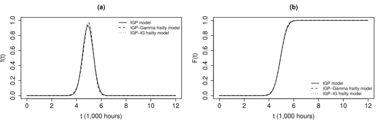
Figure 16 – (a) CDF of IGP and IGP-IG frailty models, (b) PDF of IGP and IGP-IG frailty models. . . 62
Figure 17 – 95% CPs under gamma frailty and α =0.05: (a) 95% CPs forθ, (b) 95%
CPs forη, (c) 95% CPs forα. . . 66
Figure 20 – MSEs under gamma frailty andα=0.5: (a) MSEs forθ, (b) MSEs forη, (c) MSEs forα. . . 67
Figure 21 – 95% CPs under IG fraity andα=0.05: (a) 95% CPs forθ, (b) 95% CPs for
η, (c) 95% CPs forα. . . 69
Figure 22 – 95% CPs under IG frailty andα=0.5: (a) 95% CPs forθ, (b) 95% CPs for
η, (c) 95% CPs forα. . . 70
Figure 23 – MSEs under IG frailty andα =0.05: (a) MSEs forθ, (b) MSEs forη, (c) MSEs forα. . . 70
Figure 24 – MSEs under IG fraity andα =0.5: (a) MSEs for θ, (b) MSEs for η, (c) MSEs forα. . . 71
Figure 25 – Goodness of fit test based on the LASER data: (a) IG P-P plot for degradation increments and AD test, (b) IG Q-Q plot of the degradation increments.. . . 72
Figure 26 – Degradation paths from the LASER data and expected individual frailty MLEs under different models: (a) IGP-Gamma frailty model, (b) IGP-IG frailty model. . . 74
Figure 27 – Lifetime distribution based on the LASER data: (a) Lifetime PDF, (b) Life-time CDF. . . 75
Figure 28 – Transformed degradation paths from the crack size data. . . 75
Figure 29 – Goodness of fit test based on the crack size data: (a) IG P-P plot of the degradation increments and AD test, (b) IG Q-Q plot of the degradation increments. . . 76
Figure 30 – (a) Degradation paths from the crack size data and expected individual frailty MLEs under different models: (a) IGP-Gamma frailty model, (b) IGP-IG frailty model. . . 77
Figure 31 – Lifetime distribution based on the crack size data. (a) Lifetime PDF, (b) Lifetime CDF. . . 78
Figure 32 – Degradation paths from the LASER data separated into groups. . . 87
Figure 33 – P-P plots of the degradation increments under different distributions based on the LASER data. . . 88
Figure 34 – Lifetime distribution for weak and normal groups based on the LASER data: (a) Lifetime PDF, (b) Lifetime CDF. . . 90
Figure 35 – Simulated degradation paths of 200 LASERs. . . 102
Algorithm 1 – Generating degradation paths from IGP . . . 31
Algorithm 2 – Generating degradation paths from random deterioration rate model. . . 38
Algorithm 3 – Generating degradation paths from IGP frailty model. . . 54
Table 1 – General representation of degradation data. . . 25
Table 2 – MLEs, 95% CPs and MSEs under differentσε2values. . . 43
Table 3 – MLEs, 95% CPs and MSEs under differentλ values. . . 45
Table 4 – MLEs, SEs and 95% CIs of the model parameters based on the LASER data. 47 Table 5 – AIC and BIC based on the LASER data. . . 47
Table 6 – MLEs and 95% CIs of the lifetime quantiles and MTTF based on the LASER data. . . 48
Table 7 – MLEs, SEs and 95% CIs of model parameters based on the locomotive wheels data. . . 49
Table 8 – AIC and BIC based on the locomotive wheels data. . . 49
Table 9 – MLEs and 95% CIs of the lifetime quantiles and MTTF based on the locomo-tive wheels data. . . 50
Table 10 – MLEs, 95% CPs and MSEs under gamma frailty andα =0.05. . . 65
Table 11 – MLEs, 95% CPs and MSEs under gamma frailty andα =0.5. . . 65
Table 12 – MLEs, 95% CPs and MSEs under IG frailty andα =0.05. . . 68
Table 13 – MLEs, 95% CPs and MSEs under IG frailty andα =0.5. . . 69
Table 14 – MLEs, SEs and 95% CIs of the model parameters based on the LASER data. 72 Table 15 – AIC and BIC based on the LASER data. . . 73
Table 16 – Cumulative degradation and MLEs of the expected individual frailties based on the LASER data. . . 73
Table 17 – MLEs and 95% CIs of the lifetime quantiles based on the LASER data. . . . 74
Table 18 – MLEs, SEs and 95% CIs of the model parameters based on the crack size data. 76 Table 19 – AIC and BIC based on the crack size data. . . 76
Table 20 – Cumulative degradation and MLEs of the expected individual frailties based on the crack size data. . . 77
Table 21 – MLEs and 95% CIs of the lifetime quantiles based on the crack size data. . . 78
Table 22 – MLEs of the model parameters, logL and AIC values based on the LASER data. 89 Table 23 – MLEs of the misclassification probabilities, optimal cutoff point and total cost under mixture IGP model (5.3), based on the LASER data. . . 89
Table 24 – MLEs and 95% CIs of the lifetime quantiles and MTTF based on the LASER data. . . 90
Table 27 – Estimated misclassification probabilities, optimal cutoff point and total cost
under mixture Wiener process model (5.17), based on the simulated data. . . 92
Table 28 – Estimated misclassification probabilities, optimal cutoff point and total cost under mixture gamma process model (5.18), based on the simulated data. . . 93
Table 29 – Relative bias of type I and II errors for mixture Wiener process model (5.17), based on the simulated data. . . 93
Table 30 – Relative bias of type I and II errors for mixture gamma process model (5.18), based on the simulated data. . . 94
Table 31 – MLEs of the parameters in (5.3) according to burn-in times tb, based on simulated data. . . 102
Table 32 – Estimated total cost and probabilities of type I and II errors for different values oftbands. . . 104
Table 33 – Estimated total cost for different values oftbandsundert1copula. . . 104
Table 34 – Estimated probability of type I error for different values oftbandsundert1 copula. . . 105
Table 35 – Estimated probability of type II error for different values oftbandsundert1 copula. . . 106
Table 36 – Optimal cutoff points fortb=3,000 h ands=12 undert1copula. . . 106
Table 37 – MLEs and 95% CIs of the lifetime quantiles and MTTF under differenttb values, considering simulated data. . . 107
Table 38 – LASER data (example 2.2.1) . . . 124
Table 39 – Locomotive wheels data (example 2.2.2) . . . 125
Table 40 – Crack size data (example 2.2.3) . . . 126
1 INTRODUCTION . . . 19
1.1 Introduction and bibliographical review . . . 19
1.2 Objectives of the thesis . . . 23
1.3 Organization of the chapters . . . 23
2 BACKGROUND . . . 25
2.1 Introduction . . . 25
2.2 Degradation data . . . 25
2.3 The degradation model. . . 27
2.4 Stochastic processes for degradation data . . . 28
2.4.1 The random deterioration rate model . . . 28
2.4.2 The Wiener process with drift. . . 28
2.4.3 The gamma process. . . 29
2.4.4 The inverse Gaussian process . . . 29
2.4.4.1 The inverse Gaussian distribution . . . 29
2.4.4.2 The inverse Gaussian process . . . 30
2.4.4.2.1 Distribution of the degradation increments . . . 31
2.4.4.2.2 Lifetime distribution . . . 32
2.4.4.2.3 Inference for unknown parameters in IGP model . . . 33
2.5 Frailty models . . . 34
2.6 Model selection criteria . . . 35
3 THE RANDOM DETERIORATION RATE MODEL BASED ON INVERSE GAUSSIAN DISTRIBUTION . . . 37
3.1 Introduction . . . 37
3.2 The random deterioration rate model with measurement errors . . . 37
3.2.1 Inference for unknown parameters in random deterioration rate model 38 3.2.2 Lifetime distribution. . . 40
3.2.3 IG distribution for the random deterioration rate . . . 40
3.2.3.1 Inference . . . 40
3.2.3.2 Lifetime distribution . . . 41
3.4.2 The locomotive wheels data (example 2.2.2). . . 49
3.5 Concluding remarks . . . 51
4 INVERSE GAUSSIAN PROCESS WITH FRAILTY TERM IN RE-LIABILITY ANALYSIS . . . 53
4.1 Introduction . . . 53
4.2 The IGP frailty model based on degradation increments . . . 53
4.2.1 Unconditional reliability function, CDF and PDF of the degradation increments . . . 55
4.2.2 Lifetime distribution. . . 56
4.2.3 Inference for unknown parameters in IGP frailty model . . . 57
4.2.4 Inference for individual frailties . . . 58
4.2.5 Gamma distribution for frailty . . . 58
4.2.6 IG distribution for frailty . . . 61
4.3 Simulation study . . . 64
4.3.1 Gamma distribution for frailty . . . 64
4.3.2 IG distribution for frailty . . . 68
4.4 Application . . . 71
4.4.1 The LASER data (example 2.2.1) . . . 71
4.4.2 The crack size data (example 2.2.2) . . . 75
4.5 Concluding remarks . . . 79
5 MIXTURE INVERSE GAUSSIAN PROCESS IN DEGRADATION ANALYSIS AND BURN-IN POLICY. . . 81
5.1 Introduction . . . 81
5.2 Mixture inverse Gaussian degradation process model . . . 81
5.2.1 Lifetime distribution. . . 82
5.2.2 Inference for unknown parameters . . . 82
5.3 Burn-in test and optimal burn-in time . . . 83
5.3.1 Optimal burn-in time and cutoff point . . . 84
5.4 Application - The LASER data revisited (example 2.2.1) . . . 86
5.5 Simulation study . . . 91
5.6 Concluding remarks . . . 95
6 OPTIMAL BURN-IN POLICY BASED ON A SET OF CUTOFF POINTS . . . 97
6.2 Optimal burn-in policy based on a set of cutoff points . . . 98
6.2.1 Analytical methods for determining misclassification probabilities. . . 99
6.2.2 Approximate methods using copulas for misclassification probabilities. . . 100
6.2.3 Optimal burn-in time and cutoff points . . . 100
6.3 Application . . . 101
6.3.1 The LASER data (example 2.2.1) . . . 101
6.3.2 Generated dataset . . . 101
6.4 Concluding remarks . . . 108
7 DISCUSSION, CONCLUSIONS AND FUTURE RESEARCH . . . . 109
BIBLIOGRAPHY . . . 111
APPENDIX A PROOFS OF THE THEOREMS, PROPOSITIONS AND COROLLARIES . . . 119
A.1 Proof of proposition 4.2.1 . . . 119
A.2 Proof of proposition 4.2.2 . . . 119
A.3 Proof of proposition 4.2.3 . . . 120
A.4 Proof of proposition 4.2.4 . . . 120
A.5 Proof of proposition 4.2.5 . . . 120
A.6 Proof of proposition 4.2.6 . . . 121
A.7 Proof of proposition 4.2.9 . . . 121
A.8 Proof of proposition 4.2.10 . . . 121
A.9 Proof of theorem 5.3.1 . . . 121
A.9.1 Proof of corollary 5.3.2 . . . 122
A.9.2 Proof of corollary 5.3.3 . . . 122
CHAPTER
1
INTRODUCTION
1.1
Introduction and bibliographical review
Highly reliable products present a few or no failures, then it is difficult or impossible to access reliability with traditional life tests that record only time-to-failure. However, when failure can be related directly to a quality characteristic (QC) over time, we then have the possibility of measuring degradation over time and use it to estimate the product’s reliability. It is possible to access the latent failure process characteristics and make inferences about the implied lifetime distribution. Some degradation studies consist in measuring physical degradation as a function of time (e.g., tire wear); in other applications it cannot be observed directly, but some measurements of product performance degradation (e.g., power output) may be available. Moreover, degradation analysis can have one or more variables in the underlying degradation process. Other applications of reliability prediction based on degradation modeling include reliability prediction of helicopter transmission systems, optimal degradation process control, reliability evaluation of distribution systems with aging equipment, reliability estimation of degraded structural components subject to corrosion, real-time conditional reliability prediction
from online tool performance data (WANG; COIT,2007) and degradation of nuclear power plant
components (YUAN,2007).
In reliability engineering there are two main classes of models, namely, the threshold models and the shock models; the striking difference between them is the way the failure is characterized. In the threshold models, a component reveals performance loss when its degradation level first reaches a certain threshold; this phenomenon is referred to as soft failure and the unit is usually switched off. In the shock models, a component is subject to external shocks, being able to survive or to fail; the eventual failures are referred to as hard failures or traumatic failures and the shocks usually occur according to a Poisson process whose intensity
depends on degradation and environmental factors (LEHMANN,2010). Within the class of
general path model proposed byMeeker, Escobar and Lu(1998) fits the degradation observations by a regression model with random coefficients, while the stochastic process models consider the
degradation over time as a stochastic process{D(t);t >0}to account for inherent randomness.
Gorjianet al.(2010) presented a review of degradation models, with advantages and limitations.
In the literature of the general path model, we can citeOliveira and Colosimo(2004)
that used the classical approach in automobile tyre wear data, with analytical, numerical and approximate estimation methods to obtain the time-to-failure distribution and presented some
comparisons; Peng and Tseng (2009) proposed a general linear degradation path in which
the unit-to-unit variation of all test units can be considered simultaneously with the time-dependent structure in degradation paths. They derived an explicit expression of the product’s lifetime distribution and its corresponding meantime to failure and analyzed the effects of model
misspecification on these parameters.Freitaset al. (2010) presented a comprehensive study
of various approaches for degradation data concerning the classical and Bayesian ones.Chen
and Zheng(2005) proposed an alternative method which consists in making inference directly
on the lifetime distribution itself. Zuo, Jiang and Yam (1999) introduced three approaches
for reliability modeling of continuous state devices based on the random process model, the general path model and the multiple linear regression model, respectively. They also proposed a mixture model which can be used to model both catastrophic failures and degradation failures.
Meeker, Escobar and Lu (1998) reviewed the literature concerning accelerated degradation
analysis and extended the approach ofLu and Meeker (1993) to allow for acceleration. Crk
(2000) developed a methodology based on a multiple multivariate regression model for the
component performance degradation function whose parameters may be random, correlated and
stress dependent.Chinnam(1999) used neural networks for modeling degradation signals and
Eghbali and Elsayed(2001) developed a concept of degradation rate in which the degradation hazard function is written in terms of time and degradation measure.
The random deterioration rate model is a specific stochastic model usually applied to
model corrosion and wear phenomena; seeFenyvesi, Lu and Jack (2004), EPRI(2006) and
Huyse and Roodselaar(2010). The motivation in the random variable model is to capture the randomness in the individual differences across population. This model incorporates only sample uncertainty of the degradation and no temporal variability is involved. The measurement error
models appear to work around this issue.Pandey and Lu(2013) developed a methodology for
the estimation of the growth rate parameters in noisy degradation measurement data, whose random sizing error occurs due to inspection tools. They assigned the exponential and gamma distributions to the deterioration rate, and normal distribution to the measurement errors.
Wiener process, for example,Doksum(1991) used a Wiener process with accelerating factors
to analyze degradation data,Wang(2010) presented a Wiener process with random effects for
degradation data. In the Wiener process the sample paths are not necessarily monotone, which might not be meaningful in many applications.
As an alternative, the gamma process is often adopted when monotonicity is required. The gamma process is the limit of a compound Poisson process with the jump size conforming to
a certain distribution (LAWLESS; CROWDER,2004). This interpretation underpins the gamma
process as an appropriate degradation model because many reliability engineers believe that degradation is often caused by a series of external shocks, each with random and tiny damage
(ESARY; MARSHALL,1973). The gamma process has therefore been discussed by several
authors, for example,Noortwijk(2009) made a comparative study between gamma process and
random variable models in which the first one provided advantages for taking into account the
time-dependent structure inherent in degradation data.Park and Padgett(2005) presented new
degradation models incorporating accelerating variables in stochastic processes including gamma
process and Wang (2008) proposed an estimation method grounded on the semiparametric
pseudo-likelihood for modeling degradation data through gamma process with random effects model.
Another degradation model with monotone paths is the inverse Gaussian process
intro-duced byWasan(1968) with some recent papers in the literature, for example,Wang and Xu
(2010) proposed an inverse Gaussian process with random effects and covariates to account
for heterogeneity.Ye and Chen(2014) regarded the inverse Gaussian process as the limit of a
compound Poisson process whose arrival rate goes to infinity while the jump size goes to zero in a certain way; they included a random drift in the mean function of the inverse Gaussian process,
leading to individual degradation paths with different slopes.Peng(2015) proposed a degradation
model based on an inverse normalgamma mixture of an inverse Gaussian process.Qin, Zhang
and Zhou(2013) introduced an inverse Gaussian process-based model with Bayesian approach to characterize the growth of metal loss corrosion defects on energy pipelines, wherein the
measurement errors in the paths are considered.Liuet al.(2014) developed a reliability model
for systems with s-dependent degradation processes using copulas, wherein the degradation
processes ares-dependent among each other and the marginal degradation process is modeled
by an inverse Gaussian process with time scale transformation and random drift to account for possible heterogeneity.
The frailty model is a specific approach to include randomness which allows us to incorporate the variability of the observed times coming from two distinct fonts. The first is the natural variability, which is explained by the hazard function, and the second is the common variability of the individuals from the same group or the broach variability of the several events
of the same individual, which is explained by the frailty variable.Vaupel, Manton and Stallard
model, in which the individualiwas assumed to have death intensityzih0(t)at aget where the
random variablezi(the “frailty”) is assumed to follow gamma distribution. The assumptions that
the frailty term is time independent and acts multiplicatively on an underling intensityh0(t)are
in principle arbitrary, but have been taken as the basis for much subsequent work on random heterogeneity in survival analysis. The frailty models are likely to be particularly useful for
modeling multivariate survival times, whether “serial” or “parallel” (OAKES,1989).Hougaard
(1986) pointed out the double role of the frailty distribution with finite mean in describing both
nonproportionality and interclass correlation.Unkel and Farrington(2012) provided a useful
representation of bivariate current status data to facilitate the choice of a frailty model. In the
context of degradation analysis, we can cite interesting papers, for example,Lin, Pulido and
Asplund(2014) reported an accelerated failure time (AFT) model with frailty for the analysis of
locomotive wheel’s degradation under piecewise constant hazard rate and gamma frailty; andLin
and Asplund(2014) presented a similar approach under Weibull baseline hazard rate. In these works, the lifetime information are based on the pseudo lifetimes, which are obtained when we assume some standard form for the degradation rate such as, for example, linear, exponential or power law.
Burn-in test is a technique applied to increase the quality of components and systems by testing the units before fielding them in the market. The traditional burn-in tests consist in putting the units to operate under certain conditions wherein failures are expected to occur. These tests are inefficient for highly reliable products among which even the weak units take a long time to fail. The condition-based burn-in tests arise to work around this issue, where a QC related to failure is chosen and the units with deterioration levels below a specified cutoff value are considered normal units and released to field service, whereas the ones with deterioration levels exceeding this cutoff point are considered weak ones and discarded. In the last decades, the manufacturing industry has been dedicating much effort in designing burn-in policies that eliminate latent failures before fielding them in the market. Such failures that generally occur in a small proportion among the manufactured products are caused by manufacturing defects and lead to high warranty and replacement costs. Many burn-in policies have been extensively
studied in the degradation literature; see for exampleJensen(1982),Kuo(1984) andLeemis and
Beneke(1990).
The use of mixture distributions is an important feature in burn-in policies because the components lifetime distribution is commonly bimodal from a mixture of two distributions, in which the weak units tend to fail earlier than the normal ones and the degradation values may present bimodal behavior as well. This heterogeneity is often caused either by the manufacturing process with variation of material flaws or by the fact that the components come from different suppliers. Burn-in policies are liable to misclassification errors, which are of much importance
in burn-in studies.Tseng, Tang and Ku(2003) designed an economic model based on
misclas-sification errors, and set up an optimal burn-in policy based on termination time and a set of
and Peng(2004) studied an efficient burn-in procedure based on an integrated Wiener process
for the cumulative degradation andWu and Xie(2007) suggested the use of receiver operating
characteristic (ROC) for the removal of the weak group from the production row;Tsai, Tseng
and Balakrishnan(2011) proposed a mixed gamma process for modeling degradation paths and presented an optimal burn-in policy for classifying LASER components based on a cost model.
Zhang, Ye and Xie (2015) presented a mixed inverse Gaussian process for degradation data, wherein the optimal burn-in policy to screen out the components are based on burn-time and a
single cutoff point in the decision rule.Xiang, Coit and Feng(2013) developed a burn-in policy
for preventive replacement of devices consisting ofnsubpopulations from various stochastic
processes with different degradation rates. They used mixtures of Wiener and gamma processes models and presented some comparisons.
1.2
Objectives of the thesis
The purpose of this study is to show the different methodologies for modeling degradation data. Some specific objectives are specified below:
✔ To introduce an inverse Gaussian distribution in the random deterioration rate model
with measurement errors in order to take into account the variability among different components,
✔ To introduce a frailty term in the degradation modeling in order to take into account
the unobserved heterogeneity or the dependence between the measurements of the same experimental unit, even as the presence of unobserved variables in practice,
✔ To present a decision rule for classifying a unit as normal or weak, based on burn-in time
and a set of cutoff points.
1.3
Organization of the chapters
This thesis is organized as follows.
In the second chapter we introduce the concept of degradation data and the main continu-ous processes for degradation data known in the literature, the frailty model and the selection models criteria with a brief description.
In the third chapter we propose a random deterioration rate model based on the inverse Gaussian distribution to account for both sampling and temporal variability associated with a deterioration process.
In the fifth chapter we introduce the concepts of mixture inverse Gaussian process, burn-in test and burn-in policy, where the main objective is to screen out the weak units from the normal ones in a production row. An economic model is set for determining the optimal termination time and the other parameters of a burn-in test.
In the sixth chapter we present a general and more flexible burn-in policy under the mixture inverse Gaussian process, in which the decision rule to separate the weak units from the normal ones is based on burn-in time and a set of cutoff points.
CHAPTER
2
BACKGROUND
2.1
Introduction
In this chapter, we present some features of degradation data and degradation processes in reliability analysis, followed by a brief description of frailty models and model selection criteria.
2.2
Degradation data
In a degradation test, we can observe n experimental units during a fixed period of
time. Commonly, we collect the measurements in equidistant time intervals. For each uniti, we
have the observed degradation measurements at the inspection times 0=ti0<ti1< . . . <tini,
with observationsDi(ti j),j=0,1, . . . ,ni. The vector of measurements for each unitiis called
degradation path and represented byDi≡[Di(ti1),Di(ti2), . . . ,Di(tini)]. Table1shows the general
representation of degradation data.
Table 1 – General representation of degradation data.
unit Inspection times degradation measures
1 t10=0,t11, . . . ,t1n1 D1≡[D1(t10) =0,D1(t11), . . . ,D1(t1n1)]
2 t20=0,t21, . . . ,t2n2 D2≡[D2(t20) =0,D2(t21), . . . ,D2(t2n2)]
. . . .
n tn0=0,tn1, . . . ,tnnn Dn≡[Dn(tn0) =0,Dn(tn1), . . . ,Dn(tnnn)]
In several problems the inspections 0=ti0<ti1< . . . <tini are in time scale, but other
problems exhibit the degradation in function of a variable other than the time.
The examples2.2.1,2.2.2and2.2.3exhibit some datasets in the literature. The motivation
Example 2.2.1(LASER data). Some devices for light amplification by stimulated emission,
called LASER (Light Amplification by Stimulated Emission of Radiation), present degradation over time, which results in a reduction in the emitted light. This luminosity can be maintained substantially constant with an increase in operating current. When this current reaches a very
high value, it is considered that the unit has failed.Meeker and Escobar (1998) presented a
study with degradation data of 15 LASER units from GaAs type (compound with Gallium and
Arsenic elements), with observations made up to 4,000 hours of operation, with 16 equidistant
time intervals. The degradation measure for each unit is the percent increase in current over time related to the nominal current, and a unit is considered to have failed when its degradation
measure reaches 10%. Table38in AppendixBdisplays these data and Figure1(a) shows the
corresponding degradation paths, indicating the critical value related to failure. An interesting feature of this dataset is the presence of soft failures because some components exceed the boundary but remain until the end of the experiment. Soft failures cause a performance loss but do not prevent the devices from continuing to run.
Example 2.2.2 (locomotive wheels data). Wheel failures account for much of the railroad
vehicle accidents, which lead to high costs for private companies and government. The railway maintenance services are responsible for mechanical repairs of the locomotives and hold some detailed information about preventive or corrective interventions. This dataset is part of a study
led by a Brazilian railroad company presented byFreitaset al.(2009) and containing the diameter
(in mm) of 14 locomotive wheels obtained from 13 inspections done up to 600,000 km travelled
in equidistant intervals. The degradation measure for each wheel is the wear (in mm) on the wheel diameter over the travelled distance, more specifically, the difference between the actual wheel diameter and the diameter of a new wheel (966 mm) over km travelled. A wheel is considered not be working when its degradation measure reaches 77 mm, that is, when the wheel diameter is
far 77 mm from a new wheel. Table39in AppendixBdisplays these data and Figure1(b) shows
the corresponding degradation paths, indicating the boundary related to failure. The wheels that reach the critical value remain until the subsequent inspection, when they are replaced due to preventive measures.
Example 2.2.3(fatigue crack size data). The fatigue crack size data presented byHudaket al.
(1978) was collected to obtain the fatigue cracks as a function of the number of cycles of applied
stress for 21 test specimens. The data are explored byLu and Meeker(1993) as a motivational
example in the context of nonlinear mixed effects models for degradation data. There are 21
sample paths, one for each of the 21 test units, the test stops after 0.12 million cycles and a
threshold value of 1.6 inches is set to define soft failures. Table40in AppendixBdisplays these
data and Figure1(c) shows the corresponding degradation paths, indicating the critical value
● ● ● ● ● ● ● ● ● ● ● ● ● ● ● ● ●
0 1 2 3 4
0 2 4 6 8 10 (a)
Inspections (1,000 hours)
Increase in oper
ating current (%)
● ● ● ● ● ● ● ● ● ● ● ● ● ● ● ● ● ● ● ● ● ● ● ● ● ● ● ● ● ● ● ● ● ● ● ● ● ● ● ● ● ● ● ● ● ● ● ● ● ● ● ● ● ● ● ● ● ● ● ● ● ● ● ● ● ● ● ● ● ● ● ● ● ● ● ● ● ● ● ● ● ● ● ● ● ● ● ● ● ● ● ● ● ● ● ● ● ● ● ● ● ● ● ● ● ● ● ● ● ● ● ● ● ● ● ● ● ● ● ● ● ● ● ● ● ● ● ● ● ● ● ● ● ● ● ● ● ● ● ● ● ● ● ● ● ● ● ● ● ● ● ● ● ● ● ● ● ● ● ● ● ● ● ● ● ● ● ● ● ● ● ● ● ● ● ● ● ● ● ● ● ● ● ● ● ● ● ● ● ● ● ● ● ● ● ● ● ● ● ● ● ● ● ● ● ● ● ● ● ● ● ● ● ● ● ● ● ● ● ● ● ● ● ● ● ● ● ● ● ● ● ● ● ● ● ● ● ●
critical value: 10%
● ●
● ● ● ● ● ● ● ● ● ● ●
0 100 300 500
0 20 40 60 80 100 (b)
Travelled distance (1,000 km)
Wheel diameter w
ear (mm) ● ● ● ● ● ● ● ● ● ● ● ● ● ● ● ● ● ● ● ● ● ● ● ● ● ● ● ● ● ● ● ● ● ● ● ● ● ● ● ● ● ● ● ● ● ● ● ● ● ● ● ● ● ● ● ● ● ● ● ● ● ● ● ● ● ● ● ● ● ● ● ● ● ● ● ● ● ● ● ● ● ● ● ● ● ● ● ● ● ● ● ● ● ● ● ● ● ● ● ● ● ● ● ● ● ● ● ● ● ● ● ● ● ● ● ● ● ● ● ● ● ● ● ● ● ● ● ● ● ● ● ● ● ● ● ● ● ● ● ● ● ● ● ● ● ● ● ● ● ● ● ● ● ● ● ● ● ●
critical value: 77mm
● ● ● ● ● ● ● ● ● ●
0 20 40 60 80 100
1.0 1.2 1.4 1.6 1.8 (c)
Thousands of Cycles
Cr
ack lenght (inches)
● ● ● ● ● ● ● ● ● ● ● ● ● ● ● ● ● ● ● ● ● ● ● ● ● ● ● ● ● ● ● ● ● ● ● ● ● ● ● ● ● ● ● ● ● ● ● ● ● ● ● ● ● ● ● ● ● ● ● ● ● ● ● ● ● ● ● ● ● ● ● ● ● ● ● ● ● ● ● ● ● ● ● ● ● ● ● ● ● ● ● ● ● ● ● ● ● ● ● ● ● ● ● ● ● ● ● ● ● ● ● ● ● ● ● ● ● ● ● ● ● ● ● ● ● ● ● ● ● ● ● ● ● ● ● ● ● ● ● ● ● ● ● ● ● ● ● ● ● ● ● ● ● ● ● ● ● ● ● ● ● ● ● ● ● ● ● ● ● ● ● ● ● ● ● ● ● ● ● ● ● ● ● ● ● ● ● ● ● ● ● ● ● ● ● ● ● ● ● ● ● ● ● ● ● ● ● ● ● ● ● ● ● ● ● ● ● ● ● ● ● ● ● ● ● ● ● ● ● ● ● ● ● ● ● ● ● ● ● ● ● ● ● ● ● ● ● ● ● ● ● ●
critical value: 1.6 inches
Figure 1 – (a) Degradation paths for example2.2.1, (b) Degradation paths for example2.2.2, (c) Degradation paths for example2.2.3.
2.3
The degradation model
In this work, the degradation path of a specific QC of a product is denoted byD(t), and
it is a continuous-time stochastic process{D(t),t ≥0}, that is,D(t)is a random quantity for all
t≥0.
Usually, degradation has increasing behavior over time, then the product’s lifetimeT is
suitably defined as the first passage time whenD(t)exceeds a thresholdρ, which must be fixed
in general
T =in f{t≥0|D(t)≥ρ}. (2.1)
The formula (2.1) is referred to as the first passage time distribution, which plays
an important role in predicting the remaining useful life as well as in determining optimal
maintenance strategies (NOORTWIJK,2009).
2.4
Stochastic processes for degradation data
2.4.1
The random deterioration rate model
The most simple stochastic process is defined as a time-dependent function for which
the average rate of deterioration per unit time is a random quantity (NOORTWIJK,2009). The
random deterioration rate model (or random rate model) describes the deterioration growth in a group of components using a linear function and a random parameter. Many other more complicated nonlinear models can be transformed into a linear random deterioration rate model using a time-transformation. Here we consider a simple random deterioration rate model as
D(t) =Rt≥0, withR>0, (2.2)
whereRis randomly distributed and reflects the uncertain nature of deterioration in a population
of similar components.
The random rate model presents advantages when the experiment is based on a few inspections with no measurement errors due to its easy interpretation. However, when the number of inspections is large, the individual deterioration rate surely varies with time and the inferences for the parameters are inappropriate.
2.4.2
The Wiener process with drift
The Wiener process, also known as Brownian motion, is one of the most important
stochastic processes known in the literature. Originally introduced by Brown (1828) in the
study of microscopic particles movement suspended in liquid, it has its mathematical
proper-ties explored lately byWiener(1923). The Wiener process is a continuous stochastic process
{D(t),t>0}, whose degradation path is given by
D(t) =D(0) +vt+σB(t), (2.3)
where D(0) is the starting point, v is the drift parameter, σ is the diffusion parameter and
B(t)∼N(0,t)is referred to as standard Brownian motion.
It has the following properties
- Each incrementY =∆D(t)in the time interval∆t>0 is normally distributed:
Y ∼N v∆t,σ2∆t;
- The increments are independent and stationary.
FromChhikara and Folks(1989), the first passage time (2.1) of a Wiener process with
positive drift(v>0)is inverse Gaussian distributed:
T ∼IG
ρ−D(0)
v ,
(ρ−D(0))2
σ2
In this thesis, we consider the special case whenD(0) =0, which means that the
degra-dation paths have increasing behavior starting at the origin of the coordinate system.
2.4.3
The gamma process
The gamma process is a continuous stochastic process{D(t);t≥0}with shape function
ϕψψψ(t)and scale parameterυ (NOORTWIJK,2009) given by
D(t)∼ Gamma ϕψψψ(t),υ, (2.4)
whereϕψψψ(.)is a monotone increasing function of timet indexed by the parameter vectorψψψ,
withϕψψψ(0) =0.
It holds the following properties:
- D(0) =0;
- Each incrementY =∆D(t)in the time interval∆t>0 is gamma distributed:
Y ∼ Gamma ∆ϕψψψ(t),υ,
where∆ϕψψψ(t)is the increment ofϕψψψ(.)in the time interval∆t;
- The increments are independent.
The increments are always positive with probability density function (PDF) given by
f(y) = y
∆ϕψψψ(t)−1 Γ[∆ϕψψψ(t)]υ∆ϕψψψ(t)
exp−y
υ
.
Therefore, the mean and variance of the degradation increments are given by
E(y) =∆ϕψψψ(t)υ and VAR(y) =∆ϕψψψ(t)υ2.
2.4.4
The inverse Gaussian process
First we present a brief review of the inverse Gaussian distribution.
2.4.4.1 The inverse Gaussian distribution
The inverse Gaussian (IG) distribution has its PDF given by
fIG(y|µ,λ) = s
λ
2πy3×exp
−λ(y−µ)
2
2µ2y
, (2.5)
Then we can write Y ∼ IG(µ,λ) to indicate that the random variable Y is inverse
Gaussian distributed with meanµ and shape parameterλ.
The cumulative distribution function (CDF) of the IG distribution is given by
FIG(y|µ,λ) =Φ
"s
λ y
y µ −1
#
+exp
2
λ µ
Φ
"
−
s
λ y
y µ +1
#
, (2.6)
whereΦ(.)is the standard normal CDF.
More references on theoretical results concerning the IG distribution can be found in
Seshadri(2012).
Figure2presents several scenarios for PDF and CDF of IG distribution.
0.0 0.5 1.0 1.5 2.0
0.0
0.5
1.0
1.5
2.0
(a)
y
fIG
(
y
)
µ =1, λ =1 µ =2, λ =1 µ =1, λ =2 µ =2, λ =2
0.0 0.5 1.0 1.5 2.0
0.0
0.5
1.0
1.5
(b)
y
FIG
(
y
)
µ =1, λ =1 µ =2, λ =1 µ =1, λ =2 µ =2, λ =2
Figure 2 – (a) PDF of IG distribution under different scenarios, (b) CDF of IG distribution under different scenarios.
2.4.4.2 The inverse Gaussian process
An inverse Gaussian process (IGP){D(t);t≥0}with mean functiongθθθ(t)and shape
parameterη is a continuous-time stochastic process given by
D(t)∼IG gθθθ(t),ηg2θθθ(t)
, (2.7)
wheregθθθ(.)is a monotone increasing function of timet indexed by the parameter vectorθθθ, with
gθθθ(0) =0 andη>0.
It possesses the following properties:
- D(0) =0;
- The distribution of each incrementY =∆D(t)in the time interval∆tis given by
Y ∼IG ∆gθθθ(t),η(∆gθθθ(t))2,∀∆t ≥0,
where∆gθθθ(t)ofgθθθ(t)in the time interval∆t.
The functiongθθθ(t)has a meaningful interpretation being the mean function of IGP and
η is inversely proportional to the variance of IGP:
E(D(t)) =gθθθ(t)and VAR(D(t)) =
gθθθ(t) η .
2.4.4.2.1 Distribution of the degradation increments
The CDF of the degradation incrementY in the time interval∆t is the probability ofY to
be lower thany, and come directly from CDF of IG distribution:
FIGP(y|∆gθθθ(t),η) = FIG(y|µ =∆gθθθ(t),λ =η(∆gθθθ(t))2)
= Φ
r
η
y(y−∆gθθθ(t))
+exp(2η∆gθθθ(t))Φ
−
r
η
y(y+∆gθθθ(t))
,
(2.8)
whereFIG(.)is as given in (2.6).
From (2.8) we can build up an algorithm to generate degradation paths from IGP model,
which can be modified to a simpler form when dealing with softwares like R (R Core Team,
2016) and Ox (DOORNIK,2009) which possess specific packages for generating random values
from IG distribution.
Algorithm 1 :Generating degradation paths from IGP
1 Fix values forn,gθθθ(.)andη;
2 For each uniti, (1≤i≤n):
- Setti0=0 and fix values forniandti1, . . . ,tini;
- For each index j, (1≤ j≤ni):
- Compute∆ti j =ti,j−ti,j−1and∆gθθθ(ti j) =gθθθ(ti,j)−gθθθ(ti,j−1);
- Generate a random numberui j fromU(0,1);
- Solve the nonlinear equation foryi j:FIGP(yi j|∆gθθθ(ti j),η) =ui j;
- Compute the cumulative degradation values
di1=yi1,di2=yi1+yi2. . . ,dini =yi1+. . .+yini.
Therefore, the reliability function of the degradation incrementY is interpreted as the
probability of Y to be higher than y and is given by
RIGP(y) =1−FIGP(y|∆gθθθ(t),η). (2.9)
The PDF is given by
fIGP(y|∆gθθθ(t),η) = fIG(y|µ =∆gθθθ(t),λ =η(∆gθθθ(t))2)
= r
η
2πy3∆gθθθ(t)exp
−η(y−∆gθθθ(t))
2
2y
,
where fIGis as given in (2.5).
Another important function in reliability analysis is the intensity function
hIGP(y|∆gθθθ(t),η) =
fIGP(y|∆gθθθ(t),η)
RIGP(y|∆gθθθ(t),η)
. (2.10)
Additionally, the cumulative intensity function is given by the integralHIGP(y|∆gθθθ(t),η) =
y R 0
hIGP(u|∆gθθθ(t),η)du, or equivalently
HIGP(y|∆gθθθ(t),η) =−log(RIGP(y|∆gθθθ(t),η)). (2.11)
These functions will be explored in the chapter4in the context of frailty models.
2.4.4.2.2 Lifetime distribution
Considering (2.1), the lifetime CDF is obtained directly from using the fact that the
cumulative degradationD(t)is the degradation increment in the time interval[0,t]andgθθθ(t)is
the increment of the mean function of IGP in this time interval
FTIGP(t) = 1−FIGP(y=ρ|gθθθ(t),η),whereFIGP(.)is as given in (2.8)
= Φ
−
r
η
ρ(ρ−gθθθ(t))
−exp(2ηgθθθ(t))Φ
−
r
η
ρ(ρ+gθθθ(t))
. (2.12)
An interesting property from (2.12) turns up when ηgθθθ(t) is large, which happens
for large t values, then D(t) is approximately normal with mean gθθθ(t) and variance gθθθη(t)
(CHHIKARA; FOLKS, 1989). From Tang and Chang(1995), the CDF ofT has
Birnbaum-Saunders distribution, which is a failure time model largely used in fatigue data problems (DESMOND,1985). Furthermore, the quantilestpfrom the lifetime distribution are obtained
Therefore, the lifetime PDF is given by
fTIGP(t) =
∂FTIGP(t) ∂t = φ − r η
ρ(ρ−gθθθ(t))
∂gθθθ(t) ∂t
r
η ρ
−exp(2ηgθθθ(t))Φ
−
r
η
ρ(ρ+gθθθ(t))
2
η∂gθθθ(t) ∂t
+exp(2ηgθθθ(t))φ
−
r
η
ρ(ρ+gθθθ(t))
∂gθθθ(t) ∂t
r
η
ρ, (2.13)
whereφ(.)is the standard normal PDF.
Note that (2.13) has closed form, unlike gamma process model, in which case the lifetime
PDF needs to be obtained through numerical methods; seePandey and Noortwijk(2004).
Peng(2015) obtained the meantime to failure (MTTF) from (2.13), for special case when
gθθθ(t) =θt, as
MTTF= 1
θ
rρ
ηφ(
√
ηρ) +
1
θ η + ρ θ
Φ(√ηρ)− 1
2θ η. (2.14)
2.4.4.2.3 Inference for unknown parameters in IGP model
The likelihood function fornunits being observed at the inspection timesti j,j=0, . . . ,ni
is given by
L(gθθθ(t),η) =
n
∏
i=1
ni
∏
j=1 s
η
2πy3i j∆gθθθ(ti j)exp
−η(yi j−∆gθθθ(ti j))
2
2yi j
,
where∆gθθθ(ti j) =gθθθ(ti j)−gθθθ(ti,j−1)is the observed increment of the mean function in the time
interval[tj−1,tj].
The corresponding log-likelihood function fornunits up for a constant is given by
l(gθθθ(t),η) =
m
2 log(η) +
n
∑
i=1
ni
∑
j=1
log(∆gθθθ(ti j))−
η
2 n
∑
i=1
ni
∑
j=1 yi j
+η
n
∑
i=1
ni
∑
j=1
∆gθθθ(ti j)− η
2 n
∑
i=1
ni
∑
j=1
∆gθθθ(ti j)2
yi j
, (2.15)
wherem= ∑n
i=1ni.
The maximum likelihood estimates (MLEs) of the parameters can be obtained by the
maximization of (2.15). The interval estimates for the parameters can be based on the asymptotic
normal distribution of the MLEs.
Figure3shows some simulated degradation paths from the random rate model, Wiener,
time scale is set from 0 up to 4 with 16 equidistant intervals. The shape function for the gamma
process was specified asϕψψψ(t) =ψt,ψ>0 and the mean function for the IGP was specified as
gθθθ(t) =θt,θ >0. All the parameter values are exhibited in the charts.
● ● ● ● ● ● ● ● ● ● ● ● ● ● ● ● ●
0 1 2 3 4
0 2 4 6 8 10 12 (a) t D(t) ● ● ● ● ● ● ● ● ● ● ● ● ● ● ● ● ● ● ● ● ● ● ● ● ● ● ● ● ● ● ● ● ● ● ● ● ● ● ● ● ● ● ● ● ● ● ● ● ● ● ● ● ● ● ● ● ● ● ● ● ● ● ● ● ● ● ● ● ● ● ● ● ● ● ● ● ● ● ● ● ● ● ● ● ● ● ● ● ● ● ● ● ● ● ● ● ● ● ● ● ● ● ● ● ● ● ● ● ● ● ● ● ● ● ● ● ● ● ●
µ =2, λ =45
● ● ● ● ● ● ● ● ● ● ● ● ● ● ● ● ●
0 1 2 3 4
0 2 4 6 8 10 12 (b) t D(t) ● ● ● ● ● ● ● ● ● ● ● ● ● ● ● ● ● ● ● ● ● ● ● ● ● ● ● ● ● ● ● ● ● ● ● ● ● ● ● ● ● ● ● ● ● ● ● ● ● ● ● ● ● ● ● ● ● ● ● ● ● ● ● ● ● ● ● ● ● ● ● ● ● ● ● ● ● ● ● ● ● ● ● ● ● ● ● ● ● ● ● ● ● ● ● ● ● ● ● ● ● ● ● ● ● ● ● ● ● ● ● ● ● ● ● ● ● ● ●
v=2, σ =0.6
● ● ● ● ● ● ● ● ● ● ● ● ● ● ● ● ●
0 1 2 3 4
0 2 4 6 8 10 12 (c) t D(t) ● ● ● ● ● ● ● ● ● ● ● ● ● ● ● ● ● ● ● ● ● ● ● ● ● ● ● ● ● ● ● ● ● ● ● ● ● ● ● ● ● ● ● ● ● ● ● ● ● ● ● ● ● ● ● ● ● ● ● ● ● ● ● ● ● ● ● ● ● ● ● ● ● ● ● ● ● ● ● ● ● ● ● ● ● ● ● ● ● ● ● ● ● ● ● ● ● ● ● ● ● ● ● ● ● ● ● ● ● ● ● ● ● ● ● ● ● ● ●
ψ =2, υ =0.6
● ● ● ● ● ● ● ● ● ● ● ● ● ● ● ● ●
0 1 2 3 4
0 2 4 6 8 10 12 (d) t D(t) ● ● ● ● ● ● ● ● ● ● ● ● ● ● ● ● ● ● ● ● ● ● ● ● ● ● ● ● ● ● ● ● ● ● ● ● ● ● ● ● ● ● ● ● ● ● ● ● ● ● ● ● ● ● ● ● ● ● ● ● ● ● ● ● ● ● ● ● ● ● ● ● ● ● ● ● ● ● ● ● ● ● ● ● ● ● ● ● ● ● ● ● ● ● ● ● ● ● ● ● ● ● ● ● ● ● ● ● ● ● ● ● ● ● ● ● ● ● ●
θ =2, η =10
Figure 3 – Simulated degradation paths (a) random rate model (2.2), (b) Wiener process model (2.3), (c) gamma process model (2.4), (d) IGP model (2.7).
From Figure3we can observe that the random rate model enables different degradation
slopes but does not account for temporal variability. The Wiener, gamma and IG processes show no clear difference between the degradation slopes but account for temporal variability within the paths. Moreover, the degradation paths from Wiener process can increase or decrease over time, while the paths from gamma and IG processes always grow over time.
2.5
Frailty models
In reliability analysis, incorporating the unobserved heterogeneity among experimental units is called frailty. In this thesis, the frailty term will act in the reliability of the equipments as an unobserved covariate, helping in this way to estimate the population reliability function.
Clayton(1978) introduced a frailty term in the Cox model (COX,1972) in a multiplicative
way, that is, the random variable representing the frailty,z, acts multiplicatively in the baseline
hazard functionh0(t)then
h(t|z) =zh0(t). (2.16)
In the multiplicative frailty model (2.16),zis a positive unobservable random variable
the greater the individual frailty, the greater the probability of failure (VAUPEL; MANTON;
STALLARD,1979).
The individual hazard functionh(t|z)is interpreted as the conditional hazard function
givenz. Thus, the reliability function conditional to the frailtyzis given by
R(t|z) =exp −
t Z
0
h(s|z)ds
=exp
−z
t Z
0
h0(s)ds
=exp[−zH0(t)], (2.17)
whereH0(t)is the cumulative baseline hazard function in time t.
The unconditional reliability functionR(t)is obtained by integrating (2.17) out the frailty
component by means of the frailty PDF fααα(z), indexed by the parameter vectorααα
R(t) =
∞
Z
0
R(t|z)fααα(z)dz=
∞
Z
0
exp[−zH0(t)]fααα(z)dz, (2.18)
which can be obtained by Laplace transform (ABRAMOWITZ; STEGUN,1972), stated below
Definition 2.5.1. Given a function f(x), the Laplace transform of f(x)with real argumentsis
defined as
L[f(x)](s) =
∞
Z
0
exp(−sx)f(x)dx.
Therefore, the unconditional reliability function (2.18) can be rewritten as a Laplace
transform:
R(t) =L[fααα(z)](H0(t)). (2.19)
The Laplace transform plays an important role in the context of frailty models as it
facilitates the achievement of unconditional reliability functions (WIENKE,2010). In this thesis,
the Laplace transforms are obtained through Wolfram Mathematica software (RESEARCH,
2016).
A remarkable feature in frailty models is related to its identifiability. According toElbers
and Ridder(1982), it is necessary that the distribution of the frailty term has finite expectation and the variance of the frailty term is interpreted as a measure of population heterogeneity.
Because the frailtyzis a positive random variable, we can consider different distributions such
as gamma, lognormal, IG, among others positive-valued distributions. General characteristics of
the distributions for the frailty term were studied byHougaard(1995).
2.6
Model selection criteria
The Akaike information criterion (AIC) (SAKAMOTO; ISHIGURO; KITAGAWA,1986)
and the Bayesian information criterion (BIC)(SCHWARZ,1978) are measures of relative quality
of a statistical model for a given dataset. The calculus of AIC and BIC are given by
AIC=−2 log(L) +2p,
whereLis the maximized value of likelihood function andpis the number of parameters in the
model.
BIC=−2 log(L) +plog(n),
wherenis the sample size of the study.
CHAPTER
3
THE RANDOM DETERIORATION RATE
MODEL BASED ON INVERSE GAUSSIAN
DISTRIBUTION
3.1
Introduction
In this chapter, we present the random deterioration rate model with measurement errors in order to incorporate the variability among different components. The random rate analysis is based on repeated measurements of flaw sizes created by a degradation process over time in a components population. Some features of the random rate model based on IG distribution are investigated. We conduct a simulation study to evaluate the behavior of the parameter estimators and illustrate the potentiality of the proposed model with two real-world datasets.
3.2
The random deterioration rate model with
measurement errors
In engineering problems, usually data can neither be collected nor recorded precisely due to various uncertainties such as human errors, machine errors or incomplete information (XIAOet al.,2012). Thereby, a source of variability may be added due to measurement errors.
The random deterioration rate model is explored according to the proposal fromPandey and
Lu(2013), in which a measurement error is added to the deterministic model (2.2) in order to
explain the source of variability between the measurements from the same individual path. This
model is an extension of (2.2), in which the degradation path of thei-th unit at timet is given by
Di(t) =rit+ε, (3.1)
The model (3.1) has the same formulation as the general path model (MEEKER; ES-COBAR; LU,1998), in which the main characteristic is the randomness between units.Lu and Meeker(1993) presented an approach to analyze noisy degradation data based on the nonlinear mixed effects regression model considering normal distribution with zero mean and positive
variance for the measurement errors. In this work,ε belongs to normal distribution with real
mean and positive variance:ε∼N(µε,σε2).
From (3.1) we can build up an algorithm to generate degradation paths from random
deterioration rate model given as
Algorithm 2 :Generating degradation paths from random deterioration rate model.
1 Fix values forn,µε andσε2;
2 For each uniti,(1≤i≤n):
- Setti0=0 and fix values forniandti1, . . . ,tini;
- Generate a random numberrifrom the random rate distribution (e.g. IG or gamma);
- For each index j,(1≤ j≤ni), generate a random valueεi j fromN(µε,σε2);
- Compute the degradation values:di1=riti1+εi1,di2=riti2+εi1. . . ,dini=ritini+εini.
3.2.1
Inference for unknown parameters in random deterioration rate
model
Letdi=di1,di2, . . . ,dini be the vector of degradation measurements for thei-th unit, and
the data consist ofi=1,2, . . . ,nunits, then (3.1) can be rewritten:
Di j =Di(ti j) =riti j+εi j, (3.2)
whereεi j ∼N(µε,σε2).
The analysis is based on hierarchical modeling used in Bayesian literature (KASS;
STEFFEY,1989) consisting of two stages. In the first stage, the deterioration rateriis regarded as a latent parameter whose distribution is modeled in the second stage with a hyperparameter
vectorβββ. These stages are reported below
✔ Stage 1: The vectordiis conditioned on givenriandβββ, which is seen as a latent parameter
for uniti, with distribution f(di|ri,βββ),
✔ Stage 2: Conditionally on βββ, ri constitutes an independent and identically distributed
(i.i.d.) sample from f(ri|βββ), andriandβββ are referred to as “random” and “fixed” effects,
Therefore, from conditional independence, the joint density of the data from all units,
d=d1, . . . ,dnis a product of specified densities:
f(d|βββ) = n
∏
i=1
f(di|βββ),
where the unit specific density is a marginal distribution as follows
f(di|βββ) = Z
Ri
f(di|βββ)f(ri|βββ)dri.
The hierarchical approach is coherent for analyzing noisy data and is not limited to linear degradation law.
Considering (3.2) andrifixed, the degradation measureDi j ∼N(µε+riti j,σε2). Thus the
PDF of a measured degradation is given as
f(di j|ri) = 1
√
2πσε
exp "
− di j−µε−riti j
2
2σε2
#
.
From the concept of the hierarchical modeling, the degradation measuresdi, are normally
distributed with the deterioration raterias a parameter, whileriitself has the PDF fβββ(ri).
Using the theorem of total probability, the marginal likelihood function for measurements
of ani-th unit can be written as
Li(µε,σε2,βββ) =
∞
Z
0
ni
∏
j=1
1
√
2πσε
exp
−(di j−µε−riti j)
2
2σε2
fβββ(ri)dri
=
∞
Z
0
1
√
2πσε
ni
exp "
−21
σε2
ni
∑
j=1
(di j−µε−riti j)2 #
fβββ(ri)dri
= L1i×L2i, (3.3)
where the first term inL1idoes not depend onβββ and the second termL2idepends onβββ through
the integral overri.
The likelihood function for a sample ofnindependent units is the product of the terms
L1, . . . ,Ln:
L(µε,σε2,βββ) =
n
∏
i=1
L1i×L2i.
Therefore, the corresponding log-likelihood is
l(µε,σε2,βββ) =
n
∑
i=1
log(L1i) +
n
∑
i=1
3.2.2
Lifetime distribution
Considering (2.1), the lifetime CDF is given by
FT(t) =P[D(t)≥ρ] =P[rt≥ρ] =1−FR ρ
t
, (3.5)
whereFR(.)is the deterioration rate CDF.
The quantilestpare obtained through the equationFT(t) = p.
Therefore, the lifetime PDF is obtained
fT(t) =
∂FT(t)
∂t . (3.6)
Considering the nature of degradation data, one may assume a positive-valued distribution
for the deterioration rater. In this work we assume IG distribution forr.
3.2.3
IG distribution for the random deterioration rate
We shall assume thatri’s are an i.i.d. sample from IG distribution, then we have
Di(ti j) =ri jt+εi j, whereri∼IG(µ,λ),µ>0 andλ >0, (3.7)
and the PDF for IG distribution is as given in (2.5).
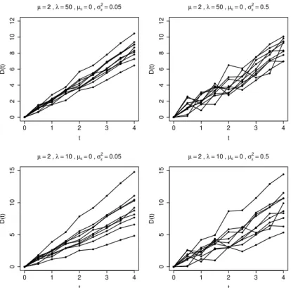
Figure4displays some degradation paths from IG random rate model (3.7) as a result of
Algorithm 2. Each chart consists of 10 units being evaluated from 0 up to 4 time units with 8 equidistant intervals. The parameter values are exhibited in the charts. We can observe that a
decrease inλ leads to an increase in the variability between the paths, while an increase inσε2
leads to an increase in the variability within the paths. Even though the paths possess increasing behavior, the model formulation allows ups and downs due to measurement errors.
3.2.3.1 Inference
The second term in (3.3) can be rewritten as
L2i=
∞
Z
0
exp "
−21
σε2
ni
∑
j=1
(di j−µε−riti j)2 #s
λ
2πr3i exp
−λ(ri−µ)
2
2µ2ri
dri, (3.8)
which is intractable analytically due to the fact that the integral does not have closed expression.
The Gaussian quadrature method arises to solve this problem. This method aims to
approximate an integral of a continuous function with respect to a quantityxonX as a weighted
sum of this function evaluated at a set of nodes (also called quadrature points):
Z
X
f(x)dx≈
Q
∑
q=1