doi: 10.1590/0101-7438.2015.035.02.0329
CLASSIFICATION OF POWER QUALITY CONSIDERING VOLTAGE SAGS IN DISTRIBUTION SYSTEMS USING KDD PROCESS
Anderson Roges Teixeira G´oes
1, Maria Teresinha Arns Steiner
2*and Rodrigo Antonio Peniche
3Received April 28, 2013 / Accepted August 28, 2014
ABSTRACT.In this paper, we propose a methodology to classify Power Quality (PQ) in distribution sys-tems based on voltage sags. The methodology uses the KDD process (Knowledge Discovery in Databases) in order to establish a quality level to be printed in labels. The methodology was applied to feeders on a substation located in Curitiba, Paran´a, Brazil, considering attributes such as sag length (remnant voltage), duration and frequency (number of occurrences on a given period of time). On the Data Mining Stage (the main stage on KDD Process), three different techniques were used, in a comparative way, for pattern recognition, in order to achieve the quality classification for the feeders: Artificial Neural Networks (ANN); Support Vector Machines (SVM) and Genetic Algorithms (GA). By printing a label with quality level in-formation, utilities companies (power concessionaires) can get better organized for mitigation procedures by establishing clear targets. Moreover, the same way costumers already receive information regarding PQ based on interruptions, they will also be able to receive information based on voltage sags.
Keywords: PQ classification, KDD Process, Artificial Neural Networks, Support Vector Machines, Genetic Algorithms, Quality Label.
1 INTRODUCTION
For better service improvement, companies from different sectors of the economy have been uti-lizing high-sensibility computerized equipments in order to improve their services. These equip-ments require good Power Quality (PQ) in order to achieve perfect function. As a result, many studies related to PQ have been developed.
Costumers demand for both products and service quality, especially when they have support from the Federal or State governments Regulatory Agencies, have led utilities companies (power
*Corresponding author.
1Federal University of Paran´a; Graduate Program in Numerical Methods in Engineering; Centro Polit´ecnico, CP. 19081; 81531-990 Curitiba, Paran´a, Brazil. E-mail: [email protected]
2Pontifical Catholic University of Paran´a; Graduate Program in Industrial and Systems Engineering; Rua Imaculada Conceic¸˜ao, 1155, Prado Velho, 80215-901 Curitiba, Paran´a, Brazil. E-mail: [email protected]
concessionaries) to look for solutions that may be able to satisfy their clients in what concerns PQ improvement and at the same time fulfill the requirements of the Brazilian Electricity Regulatory Agency (Agˆencia Nacional de Energia El´etrica, ANEEL), created in Brazil in 1997.
Many are the disturbances that occur in electric system. These disturbances, usually called “events”, can be either accidental (for example, tree branch fall; atmospheric discharges; and so on) or programmed (preventive maintenance) and they have direct influence on PQ. These events generate some PQ indicators or, also called, continuity indicators (both individual and collective), currently indicated by Brazilian utilities companies, which are related to PQ. The most outstand-ing indicators are (ANEEL, 2000): DIC index (Interruption Duration per Consumer Unit); FIC index (Interruption Frequency per Consumer Unit); DMIC (Maximum Interruption Duration per Consumer Unit); DEC index (Equivalent Interruption Duration per Consumer Unit) and FEC index (Equivalent Interruption Frequency per Consumer Unit). Among these indicators, the first three are individual indicators (per transformer) and the last two are regional indicators.
In the light of these considerations, the aim of this paper is to present a methodology that can be considered as an alternative to the fulfillment of what is proposed by ANEEL (2008). This agency has not yet defined performance standards regarding “voltage sag” events, but indicates that “concessionaires should follow up the performance of monitored bus bars and make it available on an annual basis”. This information can be a reference for the bar performance on consumer units serviced by Medium and High Voltage Distribution System with sensitive loads and short-duration voltage variations.
This study proposes a PQ classification using only three attributes: voltage sag length, duration, and frequency (number of events during a certain period). As a response to the implement of this classification, a PQ label (or quality level to be printed in labels, or simply, quality label) is generated, classifying feeders according to a six-color scale, in which each color stands for a quality level (from “A” to “F”, where “A” indicates the highest quality and “F” the lowest quality). This paper introduces an illustration of the methodology applied to feeders in a substation in the city of Curitiba, Parana, Brazil, which could be adopted and applied to other issues (G´oes, 2012).
The inspiration to create a printed label for voltage sags, in order to indicate quality level, is a result of a literature review on studies performed by Casteren et al. (2005) and Cobben & Casteren (2006). These researchers outlined a PQ classification, without, however, presenting a methodology or technique to make the PQ effective for voltage sags. Moreover, they have not worked on applications using real data, instead, they use only dummy data.
Some questions can be listed in order to direct the present research: How to use real data in order to create a quality label? How to define what “regular quality” is, based on real data? How to classify an element/pattern that does not fit any of the classification levels in the quality label? In this study we introduce a methodology, as well as its application, that answer those questions. The methodology brings in its context the Knowledge Discovery in Databases (KDD).
is answered by achieving the upper limit of the “C” range, which will be showed throughout this paper. Finally, in order to answer the third question we used three classic pattern recognition techniques: Artificial Neural Networks (ANN), Support Vector Machines (SVM) and Genetic Algorithm (GA) at the Data Mining stage (main stage of the KDD process).
This paper is organized in five sections, including this introduction. Section 2 discuss the real problem; section 3 presents a brief literature review, which indicates some studies that are re-lated to this subject; the KDD process and the Data Mining techniques used. Section 4 shows the methodology applied to the real problem and some results and finally, in Section 5, the con-clusions are presented showing the main contribution of this paper.
2 PROBLEM DESCRIPTION
Data were collected from a utility company in order to apply the developed methodology ful-filling the first aim of this research which consists in using real data to indicate the PQ. This company supplies 399 cities and 1,114 localities (districts, small towns and villages) in Parana State, Brazil and by the time of the survey it had 378 substations in order to supply around four million consumers (households, industries and others). There were 30 substations with around 300 feeders (approximately 10 feeders per substation) in the state capital city, specifically. A device is installed to detect PQ-events also measuring voltage sags in 14 of the 378 substations. Of these 14 devices, six devices are installed in substations in the capital city and its metropoli-tan area.
The methodology proposed in this study is applied to one of these substations composed of 12 feeders. However, it should be noted that this methodology can be applied to any substation as long as it has a data collector to capture the required information.
The historical records of events (voltage sags) required for the development of the proposal of this study are stored by the concessionaire in two data bases. In the first one, BD01, data are captured by the device installed in the bus bar of the substation. Each of these records contains 17 data (attributes) – “oscillographic identification”, which consists in numbering the records using a software from the concessionaire; “date and timing of the event start”, which indicates the initial time record of the PQ-related event; “type of event”, which indicates the PQ-related phenomenon: voltage sag or voltage swell, among others; and “remnant voltage or root mean square (RMS)”, which indicates the remnant voltage, in other words, the voltage “left” after the event occurrence at each of the voltage phases (Phase A, Phase B and Phase C).
The data used in the study were collected during a period of four months, between February and May 2008; BD01 was formed by 352 records (each one with 17 attributes) and BD02 was formed by 422 records (each one with 29 attributes). It is necessary to adopt a procedure in order to analyze and explore and transform this information in knowledge, thus, KDD process is used in order to explore the data that will ultimately produce the PQ label.
3 LITERATURE REVIEW
In this section, we discuss papers related to the subject here presented as well as the KDD process and an overview of techniques that were used in techniques for PQ label creation considering voltage sags.
3.1 Related Studies
There are many studies related to electrical grid disturbances (voltage sags, overvoltage, Total Harmonic Distortion, frequency, unbalanced circuits, among others) which involve many re-searches that have used Operations Research techniques in order to find the identification, loca-tion, classification and forecasting of these disturbances. Some of these researches are developed by Oleskovicz et al. (2006); Adepoju et al. (2007); Kaewarsa et al. (2008); Caciotta et al. (2009); Gencer et al. (2010); Kappor & Saini (2011) and Dash et al. (2012).
In a more detailed way, we can mention Saini & Kapoor (2012) who have conducted a review of 27 papers involving the study of signal processing (as Fourier and Wavelet transform based methods); intelligent techniques (as fuzzy logic, neural network, genetic algorithm and their fusion) and optimization techniques (Particle Swarm Optimization, Ant Colony Optimization) in PQ analysis. Tabular presentation of these 27 works has also been provided by the authors showing, mainly, the techniques applied and the data feature (synthetic or practical). Biswal et al. (2012) presented an approach for processing various non-stationary PQ waveforms through a Fast S-Transform with modified Gaussian window to generate time-frequency contours in order to extract relevant feature vectors for automatic disturbance pattern classification. The extracted features were clustered using Bacterial Foraging Optimization Algorithm (BFOA) based Fuzzy decision tree to give improved classification accuracy in comparison to the Fuzzy decision tree alone. The proposed technique was used to analyze the power signal disturbance in a realistic power network simulated by power system block set.
(2013) presented the performance evaluation of SVM with “One against All” and different clas-sification methods for PQ monitoring. The first aim was to conduct feature vector extraction and selection of PQ disturbances in a comparative way using EEMD (“Ensemble Empirical Mode Decomposition”) and EMD (“Empirical Mode Decomposition”) techniques. Feature vectors are extracted from the sampled power signals with the Hilbert Huang Transform (HHT) technique. The outputs of HHT are intrinsic mode functions (IMFs), instantaneous frequency (IF) and in-stantaneous amplitude (IA). Characteristic features are obtained from first IMFs, IF, and IA. These features were normalized along with the inputs of SVM and other classifiers.
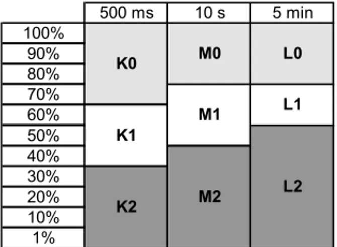
All these papers deal with “Classification of Events for Power Quality”. There is only one paper found at the literature (Casteren et al., 2005), which deals “Construction of a label for Classi-fication of Power Quality”. Casteren et al. (2005) were the first to introduce Figure 1, which was used latter by Cobben & Casteren (2006), in order to attempt to classify the voltage sags in order to indicate responsibility (consumer, equipment manufacturer or concessionaire) over the event and its mitigation measures examining the duration and the remaining value of such sags. With this data in hand Casteren et al. (2005) outlined a quality label according to frequency (number of occurrences) in order to classify voltage sags according to a table divided into nine different levels, as shown in Figure 2, grouped into three regions, where each region represents a responsibility area.
A Very high quality
B High quality
C Regular quality
D Low quality
E Very low quality
F Extremely low quality
Figure 1– PQ label. Source: Casteren et al. (2005).
500 ms 10 s 5 min 100%
90% 80% 70% 60% 50% 40% 30% 20% 10% 1%
K2 M2
L2
K0 M0 L0
K1
M1 L1
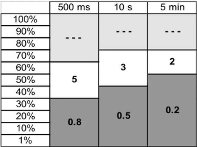
The upper region (K0, M0, L0), with duration between 500 ms and 5 min and remnant voltage between 80% and 100%, is the manufacturer’s responsibility. The intermediate region (K1, M1, L1), with analogous interpretation, is the consumer’s responsibility area. Finally, the lower re-gion (K2, M2, L2) is the concessionaire’s responsibility. The authors do not report any detailed data from the sags, either measured or simulated. Therefore, the numbers reported in the present standard criteria are dummy data. Figure 3, as an example, indicates that a costumer may prove annually a maximum of five K1 sags, three M1 sags and two L1 sags; any value higher than these would result in penalties to the concessionaires. M2 sags are allowed only once every two years.
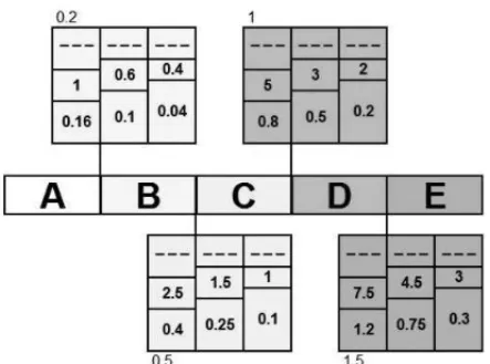
In order to facilitate the communication between consumers and concessionaires, the authors planned a classification label (quality label) of PQ based on the criteria of voltage sag character-ization, as shown in Figure 4. According to this classification “A” stands for high PQ, and “E”, for low PQ.
500 ms 10 s 5 min
100% 90%
80% 70% 60% 50%
40% 30% 20% 10%
1%
0.8 0.5
0.2 - - - - - -
-5
3 2
Figure 3– Example of criterion of characterization of voltage sags. Source: Casteren et al. (2005).
Figure 4– PQ label. Source: Casteren et al. (2005).
The classification of PQ shown in this Figure 4 must be linked to the criteria of characterization of voltage sags (Figure 3). Therefore, the authors used the upper “C” level limit criterion as shown in Figure 5. Additional criteria tables can be created analogously in order to define the upper A, B, C and D bounds.
Figure 5– PQ classification method (linking Figures 3 and 4). Source: Casteren et al. (2005).
500 ms 10 s 5 min 100%
90% 80% 70% 60% 50% 40% 30% 20% 10% 1%
0.25 0.19
0.29 - - - - - -
-2
1.1 2.3
Figure 6– Example of voltage sag events that do not fit in the framework of Figure 5. Source: Authors.
Through Figures 5 and 6, one can observe that for the values of K1=2; M1=1.1; K2=0.25; M2=0.19, the classification of the element would be “B”, but for the values of L1=2.3 and L2=0.29, the classification would be “E”. In this way, we can observe that there is not a way, at this moment, to classify this element. So, in order to classify an element of this type, we are proposing the use of SVM classifier (presented the best performance among the three techniques researched: ANN, SVM and GA), as shown throughout the paper.
3.2 KDD Process
The methodology used in this study can be framed in the context of KDD process, which aim is to find information in databases through an automated search, thus establishing interest patterns that experts may fail to observe.
The definition for KDD was first mentioned in a study performed by Frawley, Piatetsky-Shapiro & Matheus (1991), to which the authors define as “nontrivial extraction of implicit, previously unknown, and potentially useful information from data”. Three years latter Brachman & Anand (1994) defined KDD as “knowledge-intensive task consisting of complex interactions, protracted over time, between a human and a (large) database, possibly supported by a heterogeneous suite of tools”. However, the most common definition found in the literature is the one from Fayyad et al. (1995), in which KDD is “the non-trivial process of identifying valid, novel, potentially useful and ultimately understandable patterns in data”.
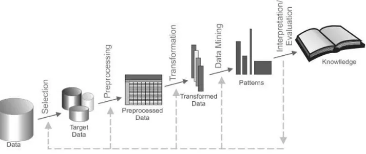
Before these concepts KDD process was often mistaken with the concept of Data Mining, which, in fact, is, within the five stages of the KDD process, the main one. These stages shown in Figure 7 are: data selection; data preprocessing; data transformation; data mining and, finally, interpretation of the knowledge generated (Fayyad et al., 1995).
Figure 7– Stages in the KDD process. Source: Fayyad et al. (1995).
It is possible to find throughout this process both explicit and non-explicit knowledge, in other words, the information can be either known information or unexpected information which was not perceived before with database analysis. There can also be information with no significant relation, due to the lack of attributes or due to the inexistence of new knowledge to be discovered. Usually the information obtained is the ones that are not detected when traditional methods of data analysis are applied for decision making. That is because most of the traditional methods are capable of verifying only the explicit information in datasets.
4 METHODOLOGY AND ITS APPLICATION
KDD process was used as the foundation of the methodology developed in this study in order to create the PQ that is basically composed of the following stages (adapted from Figure 7):
• Data Preprocessing (data cleaning and transformation);
• Association between databases (BD01 and BD02);
• Creation of the label itself. At this stage, Data Mining techniques (ANN; AG and SVM)
were used in order to achieve pattern recognition, as already mentioned;
• Result Analysis.
4.1 Data Preprocessing
At this stage of the KDD process, the attributes described in section 2 were analyzed. From BD01, where each record has 17 attributes, eight were removed and nine, which were considered relevant, left; the number of attributes of BD02 was reduced from 29 to six.
During a meeting held with the concessionaire engineers, they informed that only the records with attributes in “Type” were “Accidental” should be considered once the other two “Types” (“Programmed” and “Voluntary”) can have the PQ disturbances monitored. Once this informa-tion is exclusively for BD02, this database was filtered again and only five attributes were left, that way reducing the numbers of records from 422 to 181.
The transformation of attributes that indicate remnant voltage at each of the voltage phases was then performed in BD01. This transformation was called “aggregation of parameters”, that is, the remnant voltage of the event was defined as the lowest value among the values achieved by the three voltage phases, which was an alternative indicated by ANEEL (2008). The event duration is defined as the maximum duration between the three phase/neutral events. These values were recorded in the new “Remnant voltage” attribute, and the “RMS voltage phase A”; “RMS voltage phase B” and “RMS voltage phase C” attributes were excluded from BD01.
The methodology proposed for the creation of a feeder PQ label considered only three attributes: remnant voltage sag; sag duration, and number of occurrences. The first two attributes are in BD01 (Table 1); the third attribute is the result of a simple occurrence counting. However, BD01 does not indicate the feeder that was affected by the event once the data concerning feeders are in BD02. Thus, it is necessary to associate BD01 records with BD02 records according to a procedure introduced in the next section.
4.2 Data Association (BD01 and BD02)
Table 1– Some BD01 records after data transformation. Source: Authors.
Id. Start Start Final Final Duration
Circuit RMS
Osc. Date Time Date Time (s) (%)
9 2008-02-06 07:28:35.034 2008-02-06 07:28:35.252 218 0 60.1
10 2008-02-06 20:04:14.805 2008-02-06 20:04:14.990 185 1 35.9
. . . .
The engineers at the utility company defined the association or matching intervals for records in these databases in the following way: if a record in BD02 has the information “AR” (automatic restart) in the “Affected Component” attribute, a maximum time interval of 5 minutes in relation to a record in BD01 must be accepted, once databases record events (almost) immediately for this type of switch. In case the information is not an “AR”, but instead, other types of switches, the interval could to be up to 2 hours. In these conditions, a matching was accepted and a record in BD03 with data was created.
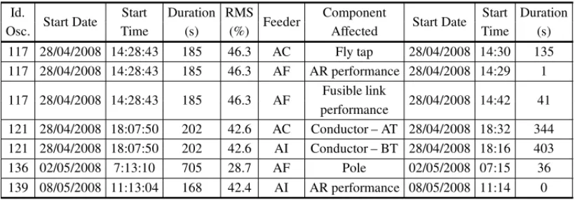
This association generated a new data base called BD03, which contains 169 records. In other words, from the 352 records in BD01 and the 181 records in BD02 there are 169 associated records matching parameter “time” accordingly to the criterion above Table 2 shows in 10 columns some examples/records of this association. Information in columns 1 to 5 is data from BD01 while columns 6 to 10 are their respective associations found in BD02. In addition, in order to identify the 12 feeders in this substation, they will be generically called AA, AB, AC,..., AK, and AL.
Table 2 shows that one record in BD01 may have more than one association with BD02 as it happens in the first three lines of the table where the “Oscillography Identification” attribute is 117. This indicates that the event captured in the substation was also “captured” or was originated in two feeders, “AC” and “AF”; where “AF” has two records for different affected components: “Fly Tap”, “AR performance”, or simply “AR” and “Fusible link performance”.
Table 2– Examples of BD03 records (association between BD01and BD02). Source: Authors.
Id.
Start Date Start Duration RMS Feeder Component Start Date Start Duration
Osc. Time (s) (%) Affected Time (s)
117 28/04/2008 14:28:43 185 46.3 AC Fly tap 28/04/2008 14:30 135
117 28/04/2008 14:28:43 185 46.3 AF AR performance 28/04/2008 14:29 1
117 28/04/2008 14:28:43 185 46.3 AF Fusible link 28/04/2008 14:42 41
performance
121 28/04/2008 18:07:50 202 42.6 AC Conductor – AT 28/04/2008 18:32 344 121 28/04/2008 18:07:50 202 42.6 AI Conductor – BT 28/04/2008 18:16 403
136 02/05/2008 7:13:10 705 28.7 AF Pole 02/05/2008 07:15 36
4.3 Creating the PQ Label for the Feeders in a Substation
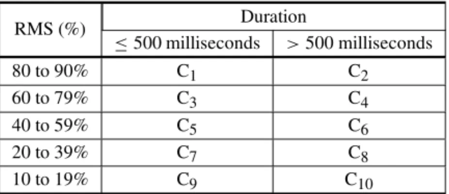
The classification for each BD03 record started with the construction of a classification table (Table 3) inspired by the proposal made by Casteren et al. (2005), as shown in Section 3.1, with the following attributes: remnant voltage sag; sag duration, and number of events. The division proposed for the Table 3 was as follows: two duration ranges were considered for the event: ≤ 500 and>500 milliseconds and five remnant voltage intervals: 10% to 19%; 20% to 39%; 40% to 59%; 60% to 79% and 80% to 90%.
Table 3– Classification considering sag duration and remnant voltage sag in the records. Source: Authors.
RMS (%) Duration
≤500 milliseconds >500 milliseconds
80 to 90% C1 C2
60 to 79% C3 C4
40 to 59% C5 C6
20 to 39% C7 C8
10 to 19% C9 C10
The connection between sag duration and remnant voltage sag can be better understood by ob-serving Table 3, where 10 possible classes, C1, C2, . . .to C10, are shown. It becomes evident that the shorter the duration, the higher the remnant voltage of the event, and the better weill bethe PQ classification for that event. Thus, the PQ of events has the following hierarchy: C1≥ C2≥. . .≥C10. In order to typify such classification, records in Table 2 are properly classified according to Table 3 and Table 4.
Table 4– Classification of records in Table 2 according to Table 3. Source: Authors.
Duration
RMS (%) Feeder Record
(milliseconds) Classification
185 46.3 AC C5
185 46.3 AF C5
185 46.3 AF C5
202 42.6 AC C5
202 42.6 AI C5
705 28.7 AF C8
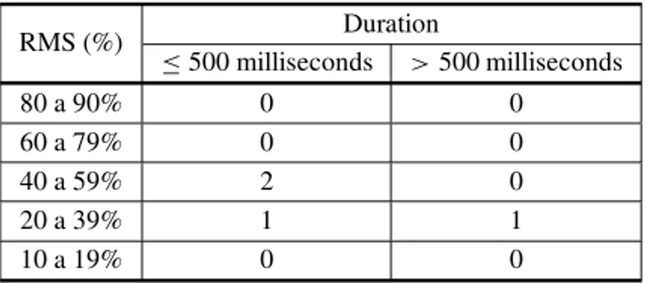
When performing this classification with the 169 records of BD03, it is assumed that the numbers of records from the “AA” feeder, for example, are the ones shown in Table 5. Record classifi-cation is achieved similarly for the other feeders in the substation. Table 5 shows that the “AA” feeder has two C5events, one C7and one C8. Table 6 considers all 169 records of all 12 feeders of the substation. It can be noted that only three of those ranges have records: C5, C7and C8.
Table 5– Classification of voltage sags of the “AA” feeder. Source: Authors.
RMS (%) Duration
≤500 milliseconds >500 milliseconds
80 a 90% 0 0
60 a 79% 0 0
40 a 59% 2 0
20 a 39% 1 1
10 a 19% 0 0
Table 6 – Classification of voltage sags in the analyzed substation, considering all the records. Source: Authors.
RMS (%) Duration
≤500 milliseconds >500 milliseconds
80 to 90% 0 0
60 to 79% 0 0
40 to 59% 149 0
20 to 39% 15 5
10 to 19% 0 0
Table 7– Average classification of voltage sags in the ana-lyzed substation. Source: Authors.
RMS (%) Duration
≤500 milliseconds >500 milliseconds
80 to 90% 0 0
60 to 79% 0 0
40 to 59% 13 0
20 to 39% 2 1
10 to 19% 0 0
In order to create the PQ label, the values of six ranges were established, where “Range A” is the best PQ and “Range F” is the worst one. For each range, some factors (defined in conjunction with the concessionaire engineers) were multiplied in order to determine the upper limit of each range. Thus, Table 7 above represents the feeder average, that is, the upper limit of “Range C”. The upper bound of “Range A” (Table 8) was obtained by multiplying values in Table 7 by 0.25.
Table 8– Upper bound of “Range A” in the PQ classification label of a feeder in a specific substation. Source: Authors.
RMS (%) Duration
≤500 milliseconds >500 milliseconds
80 to 90% 0 0
60 to 79% 0 0
40 to 59% 4 0
20 to 39% 1 1
10 to 19% 0 0
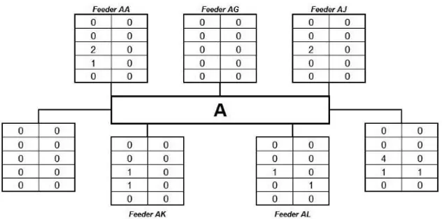
Figure 8– PQ classification label of feeders of a specific substation. Source: Authors.
Once the parameters for the label have been established, defining the lower and upper bound of occurrences for RMS intervals on each category, the classification of each feeder only requires verifying which range interval shown in Figure 8 the feeder fits in. However, it becomes evident that such task is not so simple once only five of the 12 feeders fit exactly in these ranges of values, all of them with “A” quality classification. The feeders are: AA, AG, AJ, AK and AL. The five feeders show values for C5belonging to the[0,4]interval and for C7 and C8, in the
[0,1]interval, as illustrated in Figure 9.
Other feeders could not be directly classified. In feeder AH, for example, the value of C5equals 16, which indicates that its classification would be D. However, in this feeder, C7and C8 are outside D class intervals. For that reason, in order to classify the other feeders, we used three Data Mining techniques, already briefly described in Sections 3.2.1 to 3.2.3.
4.3.1 Data Mining Techniques Application
Figure 9– Feeders classified directly from the PQ label. Source: Authors.
The techniques, used in order to classify the feeders that could not be directly classified, are the ANN, SVM, and GA according to their performance in solving the problem discussed in this paper. The specific features of these techniques are approached in A, B and C items below. Next their general features are described.
Cross-validation procedure was used in order to evaluate all the techniques, more precisely the stratified three-fold. The dataset was divided into two subsets: 2/3 for the training phase and 1/3 for testing phase. Once there is six classification ranges (“A” to “F”), each one with three RMS levels, 30 dummy records were created per range obeying the limits of each range (Figure 8), thus obtaining a total of 180 records from which 120 were used for training and 60 for testing. Since it is stratified, each set (training and testing) was formed by classes (“A” to “F”) with the same number of elements.
In addition, the training of each of the techniques occurred five times (phases), one training per class in order to identify whether the record belongs to a certain class (or not). Therefore, the training for class “A” was performed leading the technique to “learn” what is (and what is not a record from class “A”, i.e., B, C, D, E and F). Then, another training was performed for class “B”, removing the data from set “A”, and leading the technique to “learn” what is a record from class “B” (and what is not “B”, i.e., C, D, E, and F) and so on for classes “C”, “D” and “E”. When the last training was done (class “E”), if a record is not classified as “E”, it automatically becomes “F” (last class). When a new record needs to be classified, this record must be “introduced” to all the stages of the technique and its classification will be done according to the corresponding one. Following the techniques and its specific features are approached.
A. ARTIFICIAL NEURAL NETWORKS
The network was trained five times; the initial weight set varied randomly in the interval(−1,1). In total, there were 1,500 tests (three stages of the three-fold method×five classification phases – “A” to “F” –×five tests with initial weights×variation of neurons in the hidden layer 1-20). The training was done once one of the three following condition was met: 1,000 iterations; mean square error less than or equal to 10−4; or number of records incorrectly classifies as equal to zero.
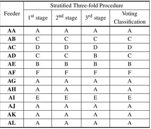
Concerning the problem discussed in this paper, the percentage of accuracy in the training of this technique was of 99.88% considering the three stages, and 99.67% in the test. Table 9 shows the result for the feeders classification obtained with the application of this technique. In Table 9, as well as in the other tables to be introduced, the “Voting Classification” column (last column) indicates the classification with the highest occurrence in the former columns, in other words, the statistical mode.
Table 9– Feeder Classification Results: ANN technique. Source: Authors.
Feeder
Stratified Three-fold Procedure
1ststage 2ndstage 3rdstage Voting Classification
AA A A A A
AB C C C C
AC D D D D
AD C C B C
AE B B B B
AF F F F F
AG A A A A
AH A A A A
AI E E E E
AJ A A A A
AK A A A A
AL A A A A
Even though the AA, AG, AJ, AK and AL feeders already have their classification defined once they were directly classified in the quality label, they were also introduced to the networks, that way confirming their classification. Therefore, six feeders have “A” classification, one feeder, “B” classification, two feeders, “C” classification, one feeder “D” classification, one feeder, “E” classification, and one feeder, “F” classification.
B. SUPPORT VECTOR MACHINES
“features space”, where it is possible to separate them linearly through one extra dimension. Therefore, even though it is not linearly separable in the pattern input space, it is in the feature space, as illustrated in Figure 10 (Vanipk, 1995, 1998; Burges, 1998).
Figure 10– Input space and feature space. Source: G´oes, 2012.
For the application of the SVM technique, it was used thesvmtrain functionof the MATLAB 7.9.0 software with the parameters: “kernel function: linear”; “optimization method: Sequential Minimal Optimization”; “tolerance to the training method: 10−3”; “parameters of the multilayer perceptron kernel:[−1,1]”.
Also, it was used with two matrices in the arguments: “Examples” and “Answers”, according to equation (1). The “Examples” matrix has the three inputsCi values (C5, C7and C8) in its columns, and the “Answer” matrix has only one column with the range value that each pattern (line of the “Examples” matrix) has as its answer (classes “A” to “F”).
Training=svmtrain(Examples, Answer) (1)
Next, a set of test, described here in the form of a matrix “NewExamples”, and the result of “Training” with thesvmclassify function, as shown in equation (2), were used in order to verify the percentage of correct classifications of these new data.
Classification=svmclassify(Training, NewExamples) (2)
It should be noted that the arguments used in the training for the svmtrain functionare the defaults on MATLAB 7.9.0 once the sets of ranges on the quality label are linearly separable by a plane. A total of 15 tests (3 training stages×5 classification phases) were performed in this technique. The accuracy percentage in the technique training was of 100%, considering the three stages of the three-fold procedure and 99.55% in the test. Table 10 shows the results of the classifications achieved with the SVM application.
Table 10– Feeder classification results: SVM technique. Source: Authors.
Feeder
Three-fold Method
1ststage 2ndstage 3rdstage Voting Classification
AA A A A A
AB C C C C
AC D C C C
AD C C B C
AE A A A A
AF F F F F
AG A A A A
AH A A A A
AI D E E E
AJ A A A A
AK A A A A
AL A A A A
C. GENETIC ALGORITHM
The GA metaheuristic was used in order to determine a plane so that in each of the semi-spaces determined by it may have only one of the sets of each stage of the application, according to the features described in the beginning of Section 4.3.1. We have to emphasize that the training sets, in the way we defined them, are linearly separable.
The value of the fitness function was established by an algorithm that determines three points that will define such plane, in which the coordinates of each point are the alleles of the individuals. Additionally, the fitness function looks for a plane equidistant to both training sets, considering the differences of the distances between two points (in different sets) that are closer to the estab-lished plane. The greater the difference between the distances, the greater the penalty applied to fitness will be.
Figure 11 shows this algorithm for the fitness calculation, where X is a vector in which each coordinate represents an allele of the individual of the population composed of nine alleles with values belonging to the set of real numbers. Thus, the three first alleles represent the coordinates of a pointP1, the next three alleles are the coordinates of point P2, and the last three are the coordinates of pointP3; C L1is the data set “class 01” (for example, “A”) andC L2is the data set “class 02” (not “A”); andkis an element that belongs toC L1∪C L2; E P(α)is the equation of the plane defined byP1,P2andP3. In this way:
i) ifk∈C L1thenkmust belong to the subspace below the planeα, and thusE P(k)should have a negative value;
iii) Dist1andDist2are initialized with high values so that algorithm determines if the plane is equidistant, or nearly equidistant, the two training sets (C L1andC L2).
For each individual X=(x1, . . . ,x9), define P1=(x1,x2,x3),P2=(x4,x5,x6)and P3=(x7,x8,x9). Correct=0;
Dist1=1000; Dist2=1000;
Determine the equation of a plane(E P(α):ax+by+cz+d=0)defined by P1, P2and P3 For each element k of the training set to be evaluated
Get the value for E P(k), replacing the k values[C5,C7,C8]in equation of the plane. Get the value for Dist, calculating the Euclidian Distance between k and the plane. If k∈C L1and E P(k) <0, then correct=correct+1;
If Dist<Dist1, then Dist1=Dist;
If k∈C L2and E P(k) >0then correct=correct+1; If Dist<Dist2, then Dist2=Dist;
z1=correct / number of examples k; z2=module (Dist1−Dist2)∗penalty; Fitness of X=z1−z2.
Figure 11– Pseudocode for fitness calculation. Source: Authors.
In Figure 11, for each individual of the GA population, it is defined a plane (P1, P2, P3) and it is verified to which subspace (determined by planeα) each elementkof the training set belong (usingE P(α)); after that, it is calculated the distance betweenkand the planeα. The value of the fitness function is determined by the difference ofz1(number of elements correctly classified) and z2 (penalty which that seeks to determine “how much” this plane is equidistant from the training sets).
For the application of the GA technique, it was used thegatoolof the MATLAB 7.9.0 software with “penality” of 0.1. The arguments for training which achieved the best results were the following: “population type: double vector”; “population size: 20”; “fitness scaling: rank”; “se-lection function: stochastic uniform”; “crossover fraction: 0.8”; “crossover function: scattered”; “stopping criteria (generations): 100”; “stopping criteria (stall generations): 50”; and “stopping criteria (function tolerance): 10−6”. It was used three stopping criteria in such a way that when a first one was reached, the procedure was finished.
It is worthwhile to remember that the “crossover scattered” works in the following way: the default crossover function creates a random binary vector and selects the genes where the vector is a “1” from the first parent, and the genes where the vector is a “0” from the second parent, and combines the genes to form the child. For example, if p1 and p2are the parents: p1 =
[abcde f gh]; p2 = [12345678]and the binary vector is[11001000], the function returns the following child[ab34e678].
of the feeders achieved through the application of this technique. The feeders AA, AG, AJ, AK and AL also confirm the classification previously achieved. Thus, there are six feeders with “A” classification, one feeder with “B” classification, four feeders with “C” classification, none with “D” classification, none with “E” classification, and one with “F” classification.
Table 11– Feeder Classification Results: GA technique. Source: Authors.
Feeder
Three-fold Method
1ststage 2ndstage 3rdstage Voting Classification
AA A A A A
AB E C C C
AC E C C C
AD B B C B
AE A A A A
AF F F F F
AG A A A A
AH E C C C
AI E C C C
AJ A A A A
AK A A A A
AL A A A A
4.4 Result Analysis
The analysis of the results is the last stage of the KDD process and it is performed in this study by comparing the classifications achieved in the three techniques that were applied. Table 12 shows the result of the achieved classification (column “voting classification” of Tables 9 to 11). In addition, this Table 12 also shows a column named “voting classification” that indicates the result of higher occurrence among the techniques, which is assumed in this analysis to be the most adequate one to solving the problem.
An analysis of Table 12 indicates that seven of the 12 feeders (AA, AB, AF, AG, AJ, AK and AL) are equally classified in all the techniques. The others achieved the same classification only in two techniques: two of them (AC and AE), with the same classification in SVM and GA techniques and three of them (AD, AH and AI), with the same classification in the ANN and SVM techniques.
Table 12– Comparison between classifications achieved through ANN, SVM and AG techniques. Source: Authors.
Feeder ANN SVM AG Voting Classification
AA A A A A
AB C C C C
AC D C C C
AD C C B C
AE B A A A
AF F F F F
AG A A A A
AH A A C A
AI E E C E
AJ A A A A
AK A A A A
AL A A A A
In the classification introduced by the ANN technique there are two feeders (AC and AE) that have different classification from the one in “voting classification”, however, in neighbor ranges. The proper classification for the AC feeder is “C”, but the ANN classified it as “D”. The AE feeder was classified by the ANN as “B” when the proper classification is “A”. Finally, SVM technique shows results that are identical to the ones from the “voting classification” column, which makes it the most adequate technique for this study.
The proper feeder classification resulted in seven feeders with “A” classification, none with “B” classification, three with “C” classification, none with “D” classification, one with “E” classifi-cation and one with “F” classificlassifi-cation. (Figure 12).
Figure 12– Quality label with feeder classification. Source: Authors.
5 CONCLUSIONS
In this work PQ classification for feeders is proposed as recommended by ANEEL. The clas-sification is assigned based on voltage sag frequencies of 10 different combinations of remnant voltage and duration. Six quality levels have been set (from “A” to “F”), and for each category there is an upper and a lower frequency for each of the 10 combinations presented on Table 3.
As there are frequencies for 10 different combinations, in several cases frequencies for a given feeder would not fit into the range for a single classification requiring additional analysis for the correct classification. For this task, based on KDD process the search for alternatives, RNA, SVM and GA metaheuristics have been used and results are compared, the best results obtained through SVM technique. The final result is an individual classification for each feeder and inscribed into a label. This label would inform PQ quality for each feeder, helping for a faster and more precise management.
Methodology has been applied for a substation unit equipped with 12 feeders. Although this number could be adequate for the study conducted here, it is strongly suggested the gathering of new information, from other sites before implementing the final classification parameters and printed labels issued.
From the results achieved in the classification of PQ considering voltage sags in distribution systems, the concessionaire will be able to analyze their performance, identifying low quality feeders and applying mitigation measures so that these feeders have their classification “lever-aged”. Therefore, this study may be continued through the identification, for example, for the reason why AF feeder has an “F” quality.
The quality label may be alternative to theANEELdemand should this methodology be applied to annual data of Power distribution substations. As already mentioned in the introduction of this study,ANEEL’s demand does not define performance patterns concerning voltage sags, but instead, it affirms that “concessionaires should follow up the performance of monitored bus bars and make them available on an annual basis”. And this information may be used as a reference to consumer units being serviced by the Distribution System.
Concerning the techniques, the SVM showed the most adequate results when compared to the “voting classification”, followed by ANN in the search for the classification of the feeders that were not directly classified in the quality label and which also classified correctly previously classified feeders. The versatility of the approached methodology allows its application in prob-lems of various fields of knowledge through many different techniques. Finally, there could be a comparison of the techniques used with others like, for example, the ones presented in Kuncheva (2004), in order to maximize the accuracy to the methodology here proposed.
6 ACKNOWLEDGEMENT
REFERENCES
[1] ADEPOJUGA, OGUNJUYIGBESOA & ALAWODEKO. 2007. Application of Neural Network to Load Forecasting in Nigerian Electrical Power System.The Pacific Jounal of Science and Technology, 8(1): 68–72.
[2] ANEEL – AGENCIAˆ NACIONAL DE ENERGIAELETRICA. 2008. Procedimentos de Distribuic¸ ˜ao´ de Energia El´etrica no Sistema El´etrico Nacional – PRODIST: M´odulo 8 – Qualidade da Energia El´etrica.
[3] ANEEL – AGENCIAˆ NACIONAL DEENERGIAEL´ETRICA. 2000. Resoluc¸˜ao no. 24, de 27 de janeiro de 2000.
[4] ANGELICO´ BA, MENDONC¸AM, ABRAO˜ T & ARRUDALV. 2013. A Comparative Analysis of three Metaheuristic Methods applied to Fuzzy Cognitive Maps Learning.Pesquisa Operacional, 33(3): 443–465.
[5] ARORAR & BHATIAR. 2012. Optimization of Automation in Fuzzy Decision Rules.Second In-ternational Conference on Advanced Computing & Communication Technologies. Haryana, ´India, p. 41–45.
[6] ATMANIB & BELDJILALIB. 2007. Knowledge Discovery in Data base: Induction Graph and Cel-lular Automaton.Computing and Informatics,26(1): 171–197.
[7] BANG J, DHOLAKIA N, HAMEL L & SHIN S. 2009. Customer Relationship Management and Knowledge Discovery in Databases.Encyclopedia of Information Science and Technology. 2nded., p. 902–907.
[8] BISWALB, BEHERAHS, BISOIR & DASHPK. 2012. Classification of power quality data using decision tree and chemotactic differential evolution based fuzzy clustering.Swarm and Evolutionary Computation,4: 12–24.
[9] BRACHMANRJ & ANANDT. 1994. The Process of Knowledge Discovery in Data bases: A First Sketch.KDD Workshop, Seattle, Washington, USA, 1–12.
[10] BRADWAJBK & PALS. 2011. Mining Educational Data to Analyze Students’Performance. Interna-tionalJounal of Advanced Computer Science and Applications,2(6): 63–69.
[11] BURGESCJC. 1998. A Tutorial on Support Vector Machines for Pattern Recognition.Data Mining and Knowledge Discovery,2(1): 121–168.
[12] CACIOTTAM, GIARNETTIS & LECCESEF. 2009. Hybrid Neural Network System for Electric Load Forecasting of Telecomunication Station.XIX IMEKO World Congress – Fundamental and Applied Metrology. Lisboa, Portugal, p. 657–661.
[13] CASTERENJFLV, ENSLINLHR, HULSHORSTWTJ, KILNGWL, HAMOENMD & COBBENJFG. 2005. A customer oriented approach to the classification of voltage dips.The 18thInternational Con-ference and exhibition on Electricity Distribution – CIRED, Turin, Italy, 1–6.
[14] COBBENJFG & CASTERENJFL. 2006. Classification Methodologies for Power Quality.Electrical Power Quality & Utilization Magazine,2(1): 11–17.
[16] DINGCH & DUBCHAKI. 2001. Multi-class protein fold recognition using support vector machines and neural networks.Bioinformatics,17(4): 349–358.
[17] FAYYADU, PIATETSKY-SHAPIROG, SMYTHP & UTHURUSAMYR. 1995. Advances in Knowledge Discovery & Data Mining. 1st. ed. American Association for Artificial Intelligence, Menlo Park, California.
[18] FRAWLEY WJ, PIATETSKY-SHAPIROG & MATHEUSCJ. 1991. Knowledge Discovery in Data bases – An Overview.Knowledge Discovery in Data bases,13(3): 1–30.
[19] GENCERO, OZTURKS & ERFIDANT. 2010. A new approach to voltage sag detection based on wavelet transform.Electrical Power and Energy Systems,32(2): 133–140.
[20] G ´OESART. 2012. Uma metodologia para a criac¸˜ao de etiqueta de qualidade no contexto de Des-coberta de Conhecimento em Bases de Dados: aplicac¸˜ao nas ´areas el´etrica e educacional.145 pages. Thesis in Numerical Methods in Engineerin, Federal University of Parana, Curitiba, Paran´a, Brazil.
[21] GOLDBERGDE. 1989. Genetic algorithms in search, optmization, and machines learning. Addison-Wesley Publishing Company, Inc. Massachusetts.
[22] HANJ & KAMBERM. 2006. Data Mining: Concepts and Techniques. 2nded. Morgan Kauffmann Publishers.
[23] HAYKINS. 1999. Neural Networks – A Comprehensive Foundation. 2nd ed. Prentice Hall, New Jersey.
[24] HOLLANDJH. 1992. Adaptation in natural and artificial systems. 2nd ed. Cambridge, USA: MIT Press.
[25] KAEWARSAS, ATTAKITMONGCOLK & KULWORAWANICHPONGT. 2008. Recognition of power quality events by using multiwavelet-based neural networks.Electrical Power and Energy Systems, 30(4): 245–260.
[26] KAPPOR R & SAINI MK. 2011. Hybrid demodulation concept and harmonic analysis for sin-gle/multiple power quality events detection and classification.Electrical Power and Energy Systems, 33(10): 1608–1622.
[27] KHEMCHANDANIR, JAYADEVA& CHANDRAS. 2009. Knowledge based proximal support vector machines.European Journal of Operational Research,195(3): 914–923.
[28] KUNCHEVALI. 2004. Combining Pattern Classifiers: Methods and Algorithms. John Wiley and Sons, Inc., New York.
[29] LIS & KUOS. 2008. Knowledge discovery in financial investment for forecasting and trading strat-egy through wavelet-based SOM networks.Expert Systems with Applications,34(2): 935–951.
[30] LIUL, QIH & LID. 2012. A research for Data Mining Technology based in Fuzzy Neural Network.
Advanced Materials Research,433-440: 2509–2512.
[31] LIUS, TIANX & ZHANGZ. 2010. Process planning knowledge discovery in the process data base. In:International Conference on Computer Application and System Modeling, Taiyuan,11(1): 370– 373.
[33] MCCULLOCHWS & PITTSW. 1943. A logical calculus of the ideas immanent in nervous activity.
Bulletin Mathematical Biology,5(4): 115–133.
[34] MITCHELLT. 1997. Machines Learning. McGraw Hill.
[35] MORAVEJZ, BANIHASHEMISA & VELAYATIMH. 2009. Power quality events classification and recognition using a novel support vector algorithm.Energy Conversion and Management,50(12): 3071–3077.
[36] OLESKOVICZ M, COURY DV, CARNEIROAAFM, ARRUDAEF, DELMONTO & SOUZASA. 2006. Estudo comparativo de ferramentas modeANNs de an´alise aplicadas `a qualidade da energia el´etrica.Revista Controle & Automac¸˜ao,17(3): 331–341.
[37] OLIVEIRAACM, CHAVESAA & LORENALAN. 2013. Clustering Search.Pesquisa Operacional, 33(1): 105–121.
[38] OZGONENELO, YALCINT, GUNEY I & KURTU. 2013. A new classification for power quality events in distribution systems.Electric Power Systems Research,9: 192–199.
[39] RODRIGUESTB, MACRINIJLR & MONTEIROEC. 2008. Selec¸˜ao de vari´aveis e classificac¸˜ao de padr˜oes por redes neurais como aux´ılio ao diagn´ostico de cardiopatia isquˆemica.Pesquisa Opera-cional,28(2): 285–302.
[40] SAINIMK & KAPOORR. 2012. Classification of power quality events – A review.Electrical Power and Energy Systems,43(1): 11–19.
[41] SASSIRJ. 2012. An hybrid architecture for clusters analysis: rough sets theory and self-organizing map artificial neural network.Pesquisa Operacional,32(1): 139–164.
[42] SETIONOR, BAESENSB & MUESC. 2009. A note on knowledge Discovery using neural networks and its application to credit card screening.European Journal of Operational Research,192(1): 326– 332.
[43] STEINERMTA, SOMANY, SHIMIZUT, NIEVOLAJC & STEINERNETOPJ. 2006. Abordagem de um problema m´edico por meio do processo de KDD com ˆenfase `a an´alise explorat´oria dos dados.
Revista Gest˜ao & Produc¸˜ao.13(2): 325–337.
[44] SUNGAH & MUKKAMALAS. 2003. Identifying important features for intrusion detection using support vector machines and neural networks.Symposium on Applications and the Internet, p. 209– 216.
[45] VAPNIKV. 1998. Statistical Learning Theory. John Wiley & Sons, Inc., New York.