doi: 10.1590/0101-7438.2017.037.02.0247
PERIODIC REVIEW SYSTEM FOR INVENTORY REPLENISHMENT CONTROL FOR A TWO-ECHELON LOGISTICS NETWORK UNDER DEMAND UNCERTAINTY: A TWO-STAGE STOCHASTIC PROGRAMING APPROACH
P.S.A. Cunha
1, F. Oliveira
1,2and Fernanda M.P. Raupp
1,3*Received August 23, 2016 / Accepted June 22, 2017
ABSTRACT.Here, we propose a novel methodology for replenishment and control systems for inventories of two-echelon logistics networks using a two-stage stochastic programming, considering periodic review and uncertain demands. In addition, to achieve better customer services, we introduce a variable rationing rule to address quantities of the item in short. The devised models are reformulated into their determin-istic equivalent, resulting in nonlinear mixed-integer programming models, which are then approximately linearized. To deal with the uncertain nature of the item demand levels, we apply a Monte Carlo simulation-based method to generate finite and discrete sets of scenarios. Moreover, the proposed approach does not require restricted assumptions to the behavior of the probabilistic phenomena, as does several existing meth-ods in the literature. Numerical experiments with the proposed approach for randomly generated instances of the problem show results with errors around 1%.
Keywords: replenishment and control systems, two-echelon logistics networks, stochastic programming, shortage rationing rules.
1 INTRODUCTION
Inventory management pervades the decision-making in many logistics networks (LNs), being thus a topic of great interest in academia. The key questions that inventory management aims to answer are how often the inventory position should be verified, when to place an order, how large an order should be, and what is the amount to keep as safety stocks in case of probabilistic demands (Namit & Chen, 1999). Maintaining safety stocks in multi-echelon LNs still lead to
*Corresponding author.
1Departamento de Engenharia Industrial, Pontif´ıcia Universidade Cat´olica do Rio de Janeiro, Rua Marquˆes de S˜ao Vicente, 225, G´avea, 22451-900 Rio de Janeiro, RJ, Brazil. E-mail: [email protected]
2School of Science, RMIT University, GPO Box 2476, Melbourne, VIC 3001, Australia. E-mail: [email protected]
other basic questions, such as, for example, what should be their amount in the entire system and how much stock should be allocated at different levels of the echelons (Axs¨ater, 2006).
A replenishment control policy establishes rules and courses of action to answer key questions relating to inventory management. In particular, it means that safety stocks can be managed in distinct ways. For example, the decision on replenishment at each facility of a LN can be based directly on stock positions or on the echelon stock level of each facility (the sum of stock positions of the facility and of all the downstream facilities in the LN). Regardless of the policy adopted, the aim is to determine the best level of inventory investment to achieve the desired service level, i.e., to guarantee a minimal percentage of demand fulfillment.
In the literature, there are several inventory policy proposals for single-echelon LNs with prob-abilistic demands. Among them, one can mention the continuous review systems (s,Q)and
(s,S), and the periodic review systems(R,S)and(R,s,S), wheresis the order point,Qis the fixed order quantity,Rrepresents the time interval between orders, andSis the maximum stock position or target level (Hadley & Whitin, 1963; Silver et al., 1998; Zipkin, 2000).
Inventory control systems with periodic review are widely used both in retail and in manufac-turing, as they require less transactional effort; involve easier planning for calculating workload needs; facilitate customer services and receiving from suppliers; allow better replenishment co-ordination, especially when they involve multiple items; and generate more stability for LNs. Furthermore, when dealing with a single-echelon LN with stationary demand, the periodic re-view yields the best results, and, in the case of a multi-echelon network, it has the advantage of being easily implementable. In the latter case, although this system is not necessarily optimal, it is capable to provide nearly optimal solutions (Federgruen & Zipkin, 1984).
In practice, besides the need for an inventory control policy, LNs with more than one echelon require the definition of a rationing rule for quantities of items in shortage. When a DC does not have sufficient stock of an item to completely and simultaneously meet all orders from retailers in a period, the rationing rule defines the shortage distribution that the DC perform to all retailers in that period.
Fair Share (FS) is the most well-known rationing rule. According to Jonsson et al. (1987), its central idea is to minimize the quantity of the item on backlog of orders (when postponements of demand fulfillment in later periods are possible) by imposing equal shortage probabilities to all retailers. To overcome this limitation, De Kok (1990) proposed the Consistent Appropriate Share (CAS), in which rationing fractions are effectively fixed based on the demands during the replenishment time at retailers, generalizing FS. However, CAS may cause imbalances or allo-cations of negative shortages, which is the case when the allocated volume of a retail shortage is greater than its order placed at the DC. Later, Van der Heijden (1997) gave an important contri-bution to the development of rationing rules, determining the rationing fractions by minimizing an imbalance average measure through the introduction of the Balanced Stock (BS) rule.
Lagodimos et al. (2008) emphasize that existing inventory modeling assumptions in the literature vary according to the rationing rule considered. Studies related to FS generally assume that the demand follows a normal distribution, while the CAS and BS rules assume either Erlang or Gamma distribution, directly affecting the developed model. While studies related to FS usually have detailed analytical models, studies related to CAS and BS are more general, requiring both numerical integration as a special approach technique, as well as optimization techniques.
Moreover, to model inventory management in a more realistic viewpoint, one can use stochastic programming as an alternative. In practice, LNs may have stochastic phenomena that depend on time-dependent market conditions, such as customer demands and prices of raw materials or freight. In fact, stochastic programming models are used when solutions of the corresponding problems are sensitive to changes in their uncertain parameters (Birge & Louveaux, 1997), and especially when the premises with respect to the probabilistic phenomena are restrictive.
According to Higle (2005), the most applied stochastic programming model is the two-stage with resource. In this technique, the first-stage variables, often referred to as design variables, correspond to those decisions that must be made before the actual realization of the uncertain parameters is observed, also known as here-and-now decisions. Then, based on these decisions and realization of random events, resource variables are considered in the second stage, which in turn are linked to control decisions, also known as wait-and-see decisions.
the quality of the representation of the stochastic phenomenon, but it is important to note that the higher the cardinality of this set, the more challenging is the problem in terms of compu-tational resources. Therefore, it is important to use appropriate techniques that allow obtaining good solutions in computational times that are acceptable in practice.
Research on LN design integrated to inventory management with uncertainty in one or more pa-rameters is relatively new. Most of the literature focuses on single-echelon LNs. Using stochastic programming, some studies already consider multi-echelon systems, as in the case of Gupta & Maranas (2000), Santoso et al. (2005), Oliveira & Hamacher (2012) and Oliveira et al. (2013). Nevertheless, despite considering inventory management and LN design jointly, these works did not address directly replenishment and inventory control policies. On the other hand, Daskin et al. (2002), Shen et al. (2003) and You & Grossmann (2008) addressed LN design and inventory policy optimization without the use of stochastic programming technique. Using stochastic pro-gramming, Fattahi et al. (2015) proposed a replenishment and inventory control methodology for a two-echelon LN in series, based on a continuous review policy(s,S), considering a single item with uncertain demand, and Cunha et al. (2017) proposed a replenishment policy for single-item single-echelon LNs with uncertain demands, with periodic review and variable order quantities in regard to ordering, holding and shortage costs.
In this paper, we present a new methodology based on two-stage stochastic programming with the use of SAA to support decision-making regarding the inventory management policy for a single item in an arborescent two-echelon LN, whose levels of demand are uncertain, over a finite time horizon. To this end, the proposed models seek to define the optimal parameters of a(R,S)control system, with periodic review and variable order quantity, to achieve minimum costs, introducing rationing fractions for quantities of the item in shortage, as well. Moreover, we performed computational experiments with generated instances to illustrate the potential of the proposed methodology.
The main contributions of this paper are detailed as follows:
1. Here we propose two-stage stochastic programming models to determine the optimal pa-rameters(R,S)of the replenishment policy for single-itemtwo-echelonLNs with a single DC and multipleretailers with uncertain demands. The deterministic equivalent models here proposed are mixed-integer nonlinear programming models, which are linearized in a novel technique.
2. Regarding the cited works of the literature that deals with the problem here addressed, we point out that in the proposed models: (a) the service levels are not considered as pre-set parameters; (b) the periodic review intervals can differ among the retailers and CD, since they are considered variables in the model; and (c) hypothesis to the stochastic phenome can be relaxed.
levels. One remarkable feature of the proposed rationing rule is that it is capable of ad-dressing negative allocations of shortage, an issue often observed when applying currently available rules.
4. Computational experiments with the proposed methodology are presented for randomly generated instances whose results are compared with the results obtained with a simulation technique.
It is worth mentioning that, in the proposed models, the relevant costs refers to ordering, carry-ing and shortage, which are considered deterministic, but possibly changcarry-ing along the planncarry-ing horizon, and the demand fulfilment being postponed if necessary (referred hereinafter as backlog case). In addition, the proposed approach does not require restrictive assumptions, such as time independence, normal distribution, nor fixed costs throughout the time horizon, to determine the optimal parameters(R,S)of the inventory policy, as well as any other assumption concerning the determination of the rationing fractions. It can thus be applied to a wider range of problems arising in this context.
In what follows, Section 2 shows the description of the problem under study. Section 3 introduces the proposed stochastic programming models to determine the optimal parameters of the control system(R,S). Section 4 briefly presents the technique used for discrete representation of random phenomenon. Section 5 presents the results of numerical experiments with instances randomly generated. Conclusion and future developments are presented in Section 6.
2 PROBLEM DESCRIPTION
Considering a single-item two-echelon LN, the problem is to define an inventory control pol-icy based on periodic review and variable order quantity under demand uncertainty, aimed at minimizing relevant costs and obtaining a desired service level. A DC and a set of retailers com-pose the arborescent distribution system. The DC places its orders to an external supplier, stores the item, and fulfills the retailers. Each retailer places its orders with the DC, stores the item and serves customers. The problem at hand does not consider costs, delays or capacities relative to transportation between the external supplier and the DC, between the DC and retailers, nor between retailers and customers.
The DC and each retaileri,i=1, . . . ,NI, adopt respectively inventory control policies(R0,S0)
Let NP be the total of periods of a given planning horizon. The review intervals, or the times between orders,R0andRi,i =1, . . . ,NI, are modeled as multiples of the period p. The lead times L0andLi,i =1, . . . ,NI, are fixed and known a priori, and are also multiples of p. The amount ordered by the DC to the external supplier is given by the difference between the target level S0and the stock position at the moment of the ordering. Likewise, each order placed by retaileriwith the DC has a required amount given by the difference between the target level Si and the stock position at the moment of the ordering. In this control system, the first order of the DC, as well as the first order of each retailer, is placed respectively at the beginning of the first period of the time horizon, which will be delivered respectively at the beginning of periods 1+L0
and 1+Li,i =1, . . . ,NI. The quantity of the item received at the beginning of a period can be consumed in the same period. Moreover, the external supplier has always sufficient stock to fulfill the DC. It is possible to store the item at all facilities, without inventory capacity limita-tions. The orders placed by the retailers with the DC, as well as the demands from the customers for the item, can be partially fulfilled, and the quantities in short are assumed to be fulfilled as soon as possible.
In the two-echelon arborescent distribution system being considered, the quantity of the item at the DC in the upstream echelon can be not sufficient to completely and simultaneously meet the demand of all retailers in the downstream echelon in a period. In this case, the decision maker must define in advance a rationing rule to be applied for distributing the shortage among the DC and retailers. To overcome this difficult, two distinct rules are considered alternatively. In the first rule, the rationing results from the application of a fixed and equal percentage to the quantities of the item in short throughout the time horizon. The second rule applies dynamically variable percentages, depending on the need of each retailer.
The relevant costs determining the optimal control parameters(R0,S0)and(Ri,Si)at DC and at each retailer i = 1, . . . ,NI, are: the carrying costs per item per period, h0p and hip, and the ordering costs CFp
0 and C
p
Fi per period, which is independent of the corresponding order quantities. Any demand that is not fully met by retaileriwill be penalized by a shortage costbip
per period, proportionally to the amount of items in short. There is no shortage cost for the case when the DC could not fully meet the amounts ordered by the retailers. The shortage cost is only applied to retailers that could not meet the customers’ demands.
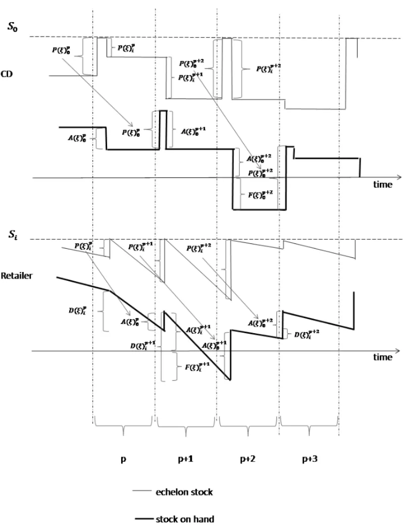
Figure 1 schematically illustrates a periodic review inventory control policy of a single item in a network with a DC and a single retailer. The lead times and the review intervals are set to
L0=L1=1 period,R0 =2 periods andR1=1 period. In this control system, the DC places
its orders with the external supplier at the beginning of periods pandp+2, denoted byP(ξ )0p
andP(ξ )0p+2, which are completely fulfilled at the beginning of periodsp+1 andp+3, since the external supplier has no capacity fulfill limitations. In turn, the retailer places its orders with the DC at the beginning of periodsp, p+1 and p+2, denoted byP(ξ )ip, P(ξ )ip+1andP(ξ )ip+2. The first two orders are completely fulfilled by the DC at the beginning of periods p+1 and
Figure 1– Scheme of the dynamics of a fixed control system.
A(ξ )0p+2, with the amount of the item in short given byF(ξ )0p+2. This backorder is then fulfilled by the DC at the beginning of periodp+4. The demands from the customers denoted byD(ξ )ip,
and p+2, and partially met in periodp+1. Hence, the retailer has a backorder in the amount
F(ξ )ip+1that will be met in period p+2.
It is worth noticing that no assumption is made on the random phenomenon driving the demand levels along the time horizon. In particular, all existing methods capable of solving the problem at hand require that the demand levels should be independent random variables and that the stochastic process should be stationary. We point out, however, that these assumptions do not need to be enforced for the applicability of the methodology proposed in this paper.
3 STOCHASTIC PROGRAMMING MODELS
In this section, we propose two-stage stochastic programming models to find the optimal param-eters of the inventory policies(R0,S0)and(Ri,Si),i = 1, . . . ,NI, related to an arborescent single-item two-echelon LN with uncertain demands, whose deterministic equivalent models are firstly formulated as mixed integer nonlinear programming (MINLP) models and then approx-imately linearized, resulting in mixed integer linear programming (MILP) models. Due to the consideration of rationing fractions for shortages in the inventory policies, a new linearization scheme is introduced based on the binary representation of decimal numbers. In the proposed models, the first-stage decisions consist of the optimal parameters (R0,S0) and (Ri,Si, fi), i = 1, . . . ,NI, where fi represents the fraction between the accumulated orders of retaileri that were not fulfilled by the DC and the accumulated orders of all retailers that were not fulfilled by the DC. The second-stage decisions are related to the optimal inventory levels and orders quantities along the time horizon, which are directly affected by the first-stage decisions and by the realization of the demand uncertainty.
Therefore, for determining the optimal parameters in the context of uncertain demands, we con-sider two distinct approaches. The first takes into account the minimization of relevant costs (ordering cost, carrying cost and shortage cost) and it is denoted byB3. In the second approach,
which is appropriated for the cases in which it is difficult to quantify the shortage cost, a condi-tion related to the demands directly fulfilled from the stocks is imposed, by defining a minimal service level by means of setting a minimal demand fraction that must be promptly fulfilled (fill rate). This approach, denoted as P2, consider the condition as a constraint in the model that minimizes the ordering and carrying costs. We remark that the notationB3andP2are consistent with that used in the literature (see, for example, Silver et al., 1998).
As follows, in Subsections 3.1 and 3.2, we present in detail the models for the problem at hand with theB3approach considering fixed and variable rationing rules. Then, in Subsection 3.3, the model with theP2approach is presented with fixed and variable rationing rules, as well.
3.1 Minimization of relevant costs with fixed rationing fractions(fi): Model B3−F
cost) and satisfy the demands while considering the balance of stocks along the time horizon. When it is not possible to completely fulfill the orders placed by the retailers in a period, it is possible to postpone the fulfillment to future periods (backlog) with the definition of a fixed-fraction rationing rule. Later, we will compare the results of this police with fixed rationing percentages with the one with variable percentages.
The model uncertainty is relative to the demand levels of the customers for the single item along the planning horizon, which are represented as random variables that follow a known continuous probability distribution. To represent the uncertain demands as discrete and finite phenomena, that is, as a number of finite scenarios with discrete values, we use a sampling technique based on the Sample Average Approximation, which will be briefly described in the following section. Hereinafter, we assume that this uncertainty representation is made available.
3.1.1 Notation
The notation used from now on for parameters and variables intends to represent the operation of the inventory control system being modelled, and so some of it could not match the usual notation that is found in the literature.
In addition to the notation previously used, we define the following:
Sets and indexes
B sizes of binary representations;t b∈ B= {1, . . . ,NB}; whereNBis the total of digits in the binary expansion (e.g., to represent 7 into binary base we need 3 digits, 111, and in this case NB =3);
I retailers,i ∈I = {1, . . . ,NI}; P time periods,p∈ P = {1, . . . ,NP};
scenarios,ξ ∈;
T0 possible review intervals at DC,r0∈T0= {1, . . . ,NR0};
Ti possible review intervals at retaileri,ri ∈Ti = {1, . . . ,NRi}; Parameters
bip unit cost of the item in short in retaileri in periodp;
CFp
0 ordering cost at DC in period p;
CFp
i ordering cost at retaileri in periodp;
D(ξ )ip demand at retaileriin scenarioξin periodp;
hip cost of carrying one unit in period pat retaileri;
h0p cost of carrying one unit in period pat DC;
S auxiliary parameter to compute the quantities of the item ordered given in terms of the upper bound for the inventory target level;
Vt b auxiliary parameter, Vt b ∈
20
10y , 2
1
10y , 2
2
10y , . . . ,2 N B
10y
and 2 >
B 2 tb
10y >1, y ∈ N∗, where 1/10y represents the desired precision (e.g., ify =1, the precision is decimal; ify =2, it is centesimal; and so forth);
wr0
0,p auxiliary parameter that indicates the period that occurs an order at DC depending on the value r0; wr00,p ∈ {0,1}; r0 = 1, . . . ,NR0;
p=1, . . . ,NP; wri
i,p auxiliary parameter that indicates the period that occurs an order at re-tailer i depending on the value ri; wri,ip ∈ {0,1}; ri = 1, . . . ,NRi;
p=1, . . . ,NP;
W auxiliaryNp×NRk matrix ofw rk
k,pparameters,k=0, . . . ,NI, defined as W = ⎛ ⎜ ⎜ ⎜ ⎜ ⎜ ⎜ ⎜ ⎜ ⎜ ⎜ ⎜ ⎜ ⎝
1 1 1 1
1 0 0 0
1 1 0 0
1 0 1 0 · · ·
1 1 0 1
1 0 0 0
1 1 1 0
.. . ⎞ ⎟ ⎟ ⎟ ⎟ ⎟ ⎟ ⎟ ⎟ ⎟ ⎟ ⎟ ⎟ ⎠ Variables
A(ξ )0p accumulated orders from all retailers fulfilled by the DC in scenario ξ
in period p, where accumulated orders refer to the orders in period p
plus all unmet orders of earlier periods;
A(ξ )ip accumulated demands met by retaileriin scenarioξin periodp, where accumulated demand stands for the demand in period pplus all unmet demands of earlier periods;
A(ξ )0p,i accumulated orders from retailers i fulfilled by DC in scenario ξ in period p;
F(ξ )0p accumulated orders from all retailers not fulfilled by DC in scenarioξ
in periodp;
F(ξ )ip accumulated demands not met by retaileri in scenarioξ in periodp;
F(ξ )0p,i accumulated orders of retaileriunmet by DC in scenarioξ in periodp;
fi shortage fraction for retailer i, that is, orders placed by retaileri not fulfilled by the DC(fi =B ji,t bVt b);
I(ξ )0p stock on hand of the DC in scenarioξ at the end of periodp;
Ie(ξ )ip echelon stock of retaileri in scenarioξat the end of periodp;
Ie(ξ )0p echelon stock of the DC in scenarioξat the end of periodp;
IIe(ξ )0p echelon stock of the DC in scenarioξat the beginning of periodp;
IIe(ξ )ip echelon stock of retaileri in scenarioξat the beginning of period p;
I VeI(ξ )0p auxiliary variable for the echelon stock of the DC in scenario ξ at the beginning of period p;
I VeI(ξ )ip auxiliary variable for the echelon stock of retaileriin scenarioξ at the beginning of period p;
J F(ξ )ip,t b auxiliary variable representing the amount of unmet orders placed by retailers in scenarioξ in periodp
ji,t b auxiliary binary variable in approximating the binary representation of fi;
P(ξ )ip quantity of the item ordered by retaileri in scenarioξ at the beginning of period p;
P(ξ )0p quantity of the item ordered by the DC in scenarioξat the beginning of period p;
SV0p auxiliary variable for the maximal inventory level of the item at DC in period p;
SVip auxiliary variable for the maximal inventory level of the item at retailer
i in periodp;
ur0
0 auxiliary binary variable for determiningR0; uri
i auxiliary binary variable in the determination ofRi;
v0p indicates if there exists an order for the item at the DC in period p;
v0p∈ {0,1};
vip indicates if there exists or not an order for the item at retaileriin period
p;vip∈ {0,1};
X(ξ )0p indicates if there exists a shortage or stock on hand at DC in scenarioξ
at the end of periodp;X(ξ )0p∈ {0,1};
3.1.2 First-stage problem
The first-stage problem is related to the decisions with respect to the review intervals R0,Ri, the target levelsS0,Si, and the fractions fi,i = 1, . . . ,NI, which must be made before the realization of uncertainty and aiming at minimizing ordering costs and the expected holding and shortage costs. The first-stage problem is formulated as follows:
minimize
p CFp
0v
p 0 +
p,i CFp
iv p
subject to r0
ur0
0 =1 (2)
ri
uri
i =1 ∀i (3)
r0
wr0
0,pu r0
0 =v p
0 ∀p (4)
ri
wri i,pu
ri i =v
p
i ∀i, p (5)
0≤S0≤ S (6)
0≤Si≤ S ∀i (7)
ur0
0,u ri
i ∈ {0,1} ∀i (8)
v0p, vip∈ {0,1} ∀i, p (9) Expression (1) models the total costs to be minimized. The first two terms refer to the sum of the costs of ordering along the planning horizon at the DC and retailers, while the third term represents the expected value of the total cost relative to second-stage problem.
Constraints (2) and (3) enforce that a single value for the review intervals R0and Ri must be determined (R0=r0∈T0= {1, . . . ,NR0}andRi =ri ∈Ti = {1, . . . ,NRi}, whenu
ro
0 =1 and uri
i =1). Constraints (4) and (5) indicate that orders occur every intervalR0at the DC and every intervalRi at retaileri, and that the first orders occur always at the beginning of the first period of the time horizon (according to the parameters valueswr0
0,pandw ri
i,p). Constraints (6) and (7) define lower and upper bounds for the variables that represent the maximal inventory levels at the DC and retailers, respectively. Note that they can be set as storage capacities available at the CD and retailers. Finally, in (8) and (9), the first-stage variablesurk
k, v p
k,k=0, . . . ,NI, are defined as binary.
3.1.3 Second-stage problem
The second-stage problem consists of minimizing the carrying and shortage costs along the time horizon facing the choices for R0,Ri,S0,Si and fi,i = 1, . . . ,NI, for a given realization of uncertain demands in each scenarioξ, to satisfy as possible the customers’ demands in all time periods. For each scenarioξ ∈, the second-stage problem is formulated as:
minimize Q(R0,Ri,S0,Si, fi, ξ )=
p
h0pI(ξ )0p+ p,i
hipI(ξ )ip+ p,i
bipF(ξ )ip (10)
subject to I(ξ )ip−1+A(ξ )p−Li
0,i =I(ξ ) p i +A(ξ )
p
I(ξ )0p−1+P(ξ )p−L0
0 =I(ξ ) p 0 +A(ξ )
p
0 ∀p≥L0 (13)
I(ξ )0p−1=I(ξ )0p+A(ξ )0p ∀p<L0 (14) Ie(ξ )ip−1+P(ξ )ip=Ie(ξ )ip+D(ξ )ip ∀p,i (15)
Ie(ξ )0p−1+P(ξ )0p=Ie(ξ )0p+ i
P(ξ )ip ∀p (16)
A(ξ )0p = i
A(ξ )0p,i ∀p (17)
F(ξ )0p = i
F(ξ )0p,i ∀p,i (18)
A(ξ )ip+F(ξ )ip=D(ξ )ip+F(ξ )ip−1 ∀p,i (19)
A(ξ )0p+F(ξ )0p= i
P(ξ )ip+F(ξ )0p−1 ∀p (20)
A(ξ )0p,i +F(ξ )0p,i = P(ξ )ip+F(ξ )0p,−i1 ∀p,i (21)
F(ξ )0p,i = fiF(ξ )0p ∀p,i (22)
P(ξ )ip =(Si−Ie(ξ )ip−1)vip ∀p,i (23) P(ξ )0p =(S0−Ie(ξ )0p−1)v0p ∀p (24)
I(ξ )0p≤ S X(ξ )0p ∀p (25)
F(ξ )0p ≤S(1−X(ξ )0p) ∀p (26)
P(ξ )ip,P(ξ )0p,A(ξ )ip,A(ξ )0p,A(ξ )0p,i,F(ξ )0p,
F(ξ )ip,F(ξ )0p,i,I(ξ )0p,I(ξ )ip,Ie(ξ )ip≥0 ∀p,i (27)
P(ξ )0i =P(ξ )00=A(ξ )i0 =A(ξ )00=F(ξ )00=
F(ξ )0i =I(ξ )00=I(ξ )0i =Ie(ξ )0i =Ie(ξ )00=0 ∀i (28)
In the objective function (10), the first two terms model the carrying costs at the DC and all retailers, which considers existing stocks on hand at the end of each periodp, while the last term represents the costs related to unmet demands by all retailers, that is, the shortage costs along the time horizon. The sum of the carrying and shortage costs is minimized over all time periods.
Constraints (17) and (18) impose the DC fulfillment to be the sum of the retailers’ fulfillment. Constraints (19), (20) and (21) model the demand fulfillment in each period for each scenario. Constraint (22) imposes that the accumulated orders of retailerinot fulfilled by the DC must be equal to the fraction fi of the accumulated orders of all retailers not fulfilled by the DC.
Constraint (23) models the order quantity of retaileri at the beginning of each period pas the target level Si minus the echelon stock of retaileri at the beginning of periodp (that coincides with the echelon stock at the end of period p−1), at the beginning of each cycle (indicated when
vip= 1); it is equal to zero, otherwise. Constraint (24) models the order quantity of the DC, at the beginning of periodp, as the target levelS0minus the echelon stock of DC at the beginning of period p(that coincides with the echelon stock at the end of period p−1), at the beginning of each cycle (indicated whenv0p=1); it is equal to zero, otherwise.
Constraints (25) and (26) indicate if the stock on hand at the DC is sufficient to fulfill the orders of the retailers. When X(ξ ) = 1, it means that all retailers’ orders are fulfilled, while, when
X(ξ )=0, at least one retailer is not fulfilled by the DC. Constraint (27) imposes non-negativity for the decision variables, while constraint (28) set their initial value to zero.
ConcerningF(ξ )0p,i in (21), we make two remarks. By definition ofF(ξ )0p,i in (22), depending on the value of fi, F(ξ )0p,i can be lower than or equal toP(ξ )ip+F(ξ )0p,−i1, and thus A(ξ )0p,i is positive and there is no imbalance (allocation of negative shortage to retailers). Otherwise, if F(ξ )0p,i is greater than P(ξ )ip+ F(ξ )0p,−i1, then A(ξ )0p,i is negative and imbalance occurs. In this case, for the proposed model to be correct it is necessary to consider the relaxation of the constraint that imposes the non-negativity for variable A(ξ )0p,i. Moreover, in case A(ξ )0p,i
is negative, this means that a shortage occurs and consequently a cost will be charged. If this consideration is not true, a solution with higher cost can be obtained in a scenario with lower probability of occurrence.
The deterministic equivalent model related to the two-stage stochastic programming problem is given by (1)-(9) and by||replications of (10)-(28). Observe that constraints from (22) to (24) turn the model to be characterized as a MINLP, which is a class of problems known as being computational challenging. Regarding constraints (23) and (24), we introduce the linearized ver-sion of the problem model as follows. First, we introduce the variablesIIe(ξ )0pandIIe(ξ )ip,∀p,i, that represent, for the DC and each retaileri, the stock position at the beginning of periodpfor given scenarioξ. AsIIe(ξ )0p= Ie(ξ )0p−1andIIe(ξ )ip = Ie(ξ )ip−1, constraints (23) and (24) are rewritten as
P(ξ )0p=SV0p−I VIe(ξ )0p ∀p (29)
P(ξ )ip=SVip−I VIe(ξ )ip ∀p,i (30)
introduction of non-negativity constraints for the auxiliary variables J F(ξ )ip,bin, SVp, IIe(ξ )0p
andI VIe(ξ )0p. Finally, the second-stage problem corresponds to the following MILP model: minimize (10)
subject to (11)-(21); (25)-(30)
SV0p≤Sv0p ∀p (31)
SVip≤Svip ∀p,i (32)
SV0p≤So ∀p (33)
SVip≤Si ∀p,i (34)
SV0p≥S0−S(1−v0p) ∀p (35)
SVip≥Si−S(1−vip) ∀p,i (36) I VIe(ξ )0p≤I T Iv0p ∀p (37)
I VIe(ξ )ip≤I T Ivip ∀p,i (38)
I VIe(ξ )0p≤IIe(ξ )0p ∀p (39)
I VIe(ξ )ip≤IIe(ξ )ip ∀p,i (40)
I VIe(ξ )0p≥IIe(ξ )0p−I T I(1−v0p) ∀p (41)
I VIe(ξ )ip≥ IIe(ξ )ip−I T I(1−vip) ∀p,i (42)
IIe(ξ )0p=Ie(ξ )0p−1 ∀p (43)
IIe(ξ )ip=Ie(ξ )ip−1 ∀p,i (44)
F(ξ )0p,i = B
Vt bJ F(ξ )ip,t b ∀p,i (45)
J F(ξ )ip,t b≤ I T I ji,t b ∀p,i,t b (46)
J F(ξ )ip,t b≤ F(ξ )0p ∀p,i,t b (47)
J F(ξ )ip,t b≥ F(ξ )0p−I T I(1− ji,t b) ∀p,i,t b (48) SV0p,SVip,I VIe(ξ )0p,I VIe(ξ )ip≥0 ∀p,i (49) As we consider stock positions at the end of periods, constraints (15) and (16) are divided into constraints (50)-(53), such that the echelon stock of retaileri in the first period is equal to the target levelSiminus the average demand per period, and that the echelon stock of the DC in the first period is equal to the target levelS0minus the sum of the average demand of the retailers, as follows:
Si−µi =Ie(ξ )ip ∀p=1,∀i (51) Ie(ξ )0p−1+P(ξ )0p=Ie(ξ )0p+
i
P(ξ )ip ∀p≥2 (52)
S0− i
µi =Ie(ξ )0p ∀p=1 (53)
Moreover, the order of retaileri not fulfilled by DC, denoted by F(ξ )0p,i, must be equal to the
corresponding orderP(ξ )ipplus the quantity in short in the earlier periodF(ξ )0p,−i1duringL0:
F(ξ )0p,i = P(ξ )ip+F(ξ )0p,−i1 ∀p≤L0; ∀i (54)
3.2 Minimization of relevant costs with variable rationing fractions(f(ξ )ip): ModelB3−V
An alternative for rationing the quantity in short among the retailers is to set a fraction based on the retailers’ needs (accumulated unmet orders) for each period and each scenario, f(ξ )ip. Thus, model B3−V differs from modelB2−F with respect to first-stage decisions. While in model B3−F, the fraction fiis a first-stage decision, in modelB3−V the fraction f(ξ )ipcan be revised in the second stage. Therefore, we rewrite constraint (22) as (55) to model the variable-fractions rationing rule:
F(ξ )0p,i = f(ξ )ipF(ξ )0p ∀p,i (55) where
f(ξ )ip= P(ξ ) p i +F(ξ )
p−1 0,i
i P(ξ ) p i +F(ξ )
p−1 0,i
= N ec(ξ ) p i
N ec(ξ )p, (56) andN ec(ξ )prepresents the sum of all the retailers’ demands until periodpandN ec(ξ )ip repre-sents the demand of retaileriuntil periodp.
3.2.1 Notation
Consider also the following notation:
Variables
di f(ξ )p auxiliary variable to computeF(ξ )ip
f(ξ )ip fraction between the need of retaileri and the needs of all retailers until periodpof scenarioξ;
L F(ξ )ip,t b auxiliary variable for the amount of unmeet orders placed by retailers in scenarioξ in periodp;
l(ξ )ip,t b auxiliary binary variable for the approximation of the binary representation of f(ξ )ip;
N ec(ξ )p total of all retailers’ demands until periodp;
N ec(ξ )ip demand of retaileriuntil periodp;
Using the binary expansion and a predefined precision of 1/10y, whereyis a fixed known value, we observe that f(ξ )ipis in the following interval:
B
Vt bl(ξ )ip,t b ≤ f(ξ ) p i ≤
B
Vt bl(ξ )ip,t b+ 1
10y (57)
As the approximate value given by the binary expansion
BVtbl(ξ ) p
i,t bof the fraction f(ξ ) p i is always less than or equal to the corresponding true value plus the precision term, on the right-hand side of the inequality (57), thus
BVtbl(ξ )ip,t brelated to all retailers will often be less than 1. To overcome this drawback, the difference
di f(ξ )p=1− i
B
Vt bl(ξ ) p i,t b
is rationed equally among all retailers.
From (56), we note thatVt bl(ξ )ip,t b considers the need of each retailer and thus a new binary representation is proposed:
B
Vt bN ec(ξ )pl(ξ )ip,t b ≤N ec(ξ )ip≤
B
Vt bN ec(ξ )pl(ξ )ip,t b+
N ec(ξ )p
10y (58)
AsN ec(ξ )pl(ξ )ip,t b=L N ec(ξ )ip,t bandF(ξ )0pl(ξ )ip,t b =L F(ξ )ip,t b, it follows that:
B
Vt bL N ec(ξ )ip,t b ≤N ec(ξ )ip≤
B
Vt bL N ec(ξ )ip,t b+
N ec(ξ )p
10y (59)
F(ξ )0p,i = B
Vt bL F(ξ )ip,t b+
F(ξ )0p− i
B
Vt bL F(ξ )ip,t b
NI (60)
Thus, the approximate linearization of constraint (55) results in its substitution by the expres-sions (61) to (68):
B
Vt bL N ec(ξ )ip,t b ≤ N ec(ξ ) p
i ∀p,i (61)
N ec(ξ )ip ≤ B
Vt bL N ec(ξ )ip,t b+
N ec(ξ )p
10y ∀p,i (62)
L N ec(ξ )ip,t b ≤Sl(ξ )ip,t b ∀p,i,t b (63)
L N ec(ξ )ip,t b≥ N ec(ξ )p−S(1−L(ξ )ip,t b) ∀p,i,t b (65)
L F(ξ )ip,t b≤Sl(ξ )ip,t b ∀p,i,t b (66)
L F(ξ )ip,t b≤ F(ξ )0p ∀p,i,t b (67)
L F(ξ )ip,t b≥ F(ξ )0p−S(1−l(ξ )ip,t b) ∀p,i,t b (68)
3.3 Minimization of costs with level service condition: ModelP2
In this approach, the objective is to minimize the ordering and carrying costs along the time horizon with the additional condition on the minimum service level, that is, the requirement that the average demand fulfillment is greater than or equal to a pre-set value given by the decision maker.
The first-stage problem is equal to the corresponding model of approachB3, except for the
short-age cost that is removed from the objective function. Thus, the second-stshort-age problem model has the following additional constraints for a given scenarioξ:
p,ξ
Pr(ξ )F′(ξ )ip p,ξ
D(ξ )ip≤1− ¯fi ∀i (69)
I(ξ )ip≥ ¯S X(ξ )ip ∀p,i (70)
F(ξ )ip≥ ¯S(1−X(ξ )ip) ∀p,i (71) where f¯i is the expected value of the fractions of the demands of retaileripromptly fulfilled and F′(ξ )ip=
pF(ξ ) p i −
pF(ξ ) p−1
i , and, as already defined, X(ξ ) p
i indicates if there is or not shortage or stock on hand at retaileriat the end of periodp.
For this approach, the fixed and variable rationing rules are considered, resulting into the models named asP2−F andP2−V, respectively.
4 SAMPLING TECHNIQUE
Probabilistic parameters that follow continuous distributions impose some difficult in solving stochastic optimization problems. In particular, in the addressed problem the difficult is associ-ated to the evaluation of the first-stage objective function (1) given in general terms by
ϕ(R,S, f)+E[Q(R,S, f, ξ )] (72)
whereis the finite set of scenarios of the demands at retailers along the time horizon, with
for a problem instance composed by M subsets of N scenarios, which are successively and independently sampled.
Thus, for each subsetM, the first-stage objective function can be approximated by the following problem:
ˆ
gN =minimize
ϕ(R,S, f)+ 1 N
n=1,...,N
QR,S, f, ξn
, (73)
where Q(R,S, f, ξn)is the objective function of the second-stage problem to be evaluated in each subsetMand scenarioξn. Given a collection of subsets of scenarios independently gener-ated by sampling(ξ1j, . . . , ξjN),j =1, . . . ,M, we have:
ˆ
gNj =minimize
ϕ(R,S, f)+ 1 N
n=1,...,N
QR,S, f, ξnj
, (74)
where the value of the first-stage objective function is approximated by:
ˆ gN,M =
1
M M
j=1
ˆ
gNj (75)
According to Santoso et al. (2005), the expected valuegˆN is less than or equal to the minimal optimal value and, sincegˆN,M is a biased estimator of the expected valuegˆN, the expected value
ˆ
gN,M is also less than or equal to the minimal optimal value of the problem. Hence, with this technique we can consider the minimal optimal value obtained as a lower bound (LB) of the optimal value of the original objective function.
Choosing good feasible first-stage solutions(R′,S′, f′), the objective function value of the first-stage model can be approximated by:
ˆ
ϕN′ =ϕ(R′,S′, f′)+ 1 N′
n=1,...,N′
Q(R′,S′, f′, ξn) (76)
Givenξ1j′, . . . , ξjN′′, j′=1, . . . ,M′, we have:
ˆ
ϕNj′′ =ϕ(R′,S′, f′)+
1
N′
n=1,...,N′
Q(R′,S′,f′, ξnj′) (77)
and thus,
ˆ
ϕN′,M′ = 1 M′
M′
j′=1
ˆ
ϕNj′ (78)
Santoso et al. (2005) also state that ϕˆN′ is an unbiased estimator for ϕ(Rˆ ′,S′, f′). Since (R′,S′, f′)is a feasible solution of the problem, ϕ(Rˆ ′,S′, f′)is greater than or equal to the minimal value of the problem. And, since ϕˆN′,M′ is an unbiased estimator for ϕˆN′,ϕˆN′,M′ is
also greater than or equal to the optimal minimum value of the problem. Thus, ϕˆN′,M′ can be
considered as an upper bound (UB) for the optimal minimum value of the original objective function.
Linderoth et al. (2006) show that with this technique we can obtain lower and upper bounds of the optimal value and that such bounds converge to the optimal value asN increases.
From the Central Limit Theorem, the confident interval for LB and UB, with levelα, where
P(z≤zα)=1−α, could be expressed respectively as
L B−z√ασL B M , L I+
zασL B √
M
and
U B−z√ασU B M′ , L S+
zασU B √
M′
,
whereσL B2 andσU B2 are respectively the variance estimators of LB and UB. Besides the obtained bounds, the estimates of the optimality gap and its variance are:
gap=U B−L B and σga p2 =σL B2 +σU B2 .
There are many ways to estimate the number of scenarios in order to obtain an approximation of the optimal value with a certain margin of error (Kleywegt et al., 2002; Shapiro and Homem-de-Melo, 1998). One of them is to use some of the ideas of the sampling technique, which gives statistical basis to get the number of scenarios.
To this end, we have from (74) thatgˆN is the minimal expected value of the objective function, which is a random variable. Moreover, gˆN is also an estimator for the minimal value of the objective function. Thus, for each scenario of{ξ1, ξ2, . . . , ξN}, we have, forn =1, . . . ,N, that the expected values of the deterministic objective function values are:
gN(ξj)=minimize{ϕ(R,S, f)+Q(R,S, f, ξn)} (79) with variance given by:
ˆ
σN =
N
n=1(gˆN− ˆgN(ξn))2
N−1 (80)
From the Central Limit Theorem, we define a confident interval with levelα/2 for the estimator ˆ
gN:
ˆ gN−
zα/2σˆN √
N , gˆN+ zα/2σˆN
√
N
Now, using the reverse form of this interval, an estimate for the lower bound of the number of scenarios needed in the approximation of the objective function is
N ≥
z α/2σˆN (β/2)gˆN
2
whereβ ∈ [0,1]. Besides the theoretical result stated in (81), in practice, the determination of the number of scenarios should consider the trade-off between the computational effort and the quality desired for the solution.
5 NUMERICAL EXPERIMENTS
In this section, we show two computational experiments conducted with the proposed stochas-tic programing models for randomly generated instances. The two-stage stochasstochas-tic programming models and the sampling technique were implemented using AIMMS version 3.13, and the corre-sponding MILP models were solved using CPLEX version 12.5. We performed the experiments in an AMD Duo-Core 1.9 GHz processor with 4 GB RAM.
The first computational experiment is conducted with B3 − F model, which minimizes the
relevant costs, including the shortage cost and considering the fixed-fractions rationing rule. To this purpose, we generated instances for the problem with 1 DC and 3 retailers, with pa-rameters values set to: NR0 = 3, r0 ∈ {1,2,3}, NRi = 1, ri = 1, ∀i, C
p
F0 = 200 and
L0 =Li =1, ∀i. Also, the costs of carrying per unit of the item in period pareh0p =1, ∀p, andhip=4, ∀i,p; and the shortage cost per unit of the item per period isbip=10, ∀i,p. In this experiment, the Nvalue was defined according to (81). Therefore, for a 5% confidence interval, we setα=0.05 andβ =0.1. Then, to get an approximation of the objective function value we consideredN =50σ50, withgˆN =298.89 andσˆN =17.52, resulting inN >5.28. Assuming that a stationary stochastic process of second order represents the demands for the item along the periods, theNscenarios were generated as follows:
D(ξ )p=a+εp, ∀p, ∀ξ (82) whereais the (constant) demand level andεpis the error associated to the model at each period, which follows a normal distribution with zero average and varianceσ2. For each scenarioξ and for all the periods of the time horizon, the demands for the item of the retailers follow a normal distribution with mean 27, 81 and 54, respectively, and variance 23, 39 and 31, respectively, having 54 as reference for the mean (54/2,(3/2)54 and 54) and 31 as reference for the variance (31−8, 31+8 and 31). The demands along the periods of each retailer follow identical probability distributions, without correlations among them.
To obtain the lower bound (LB), as in (75), for the approximation of the objective function we performed 10 runs(M =10)considering 10 scenarios(N = 10)and 20 periods(NP =20), which showed to be sufficient to observe in all runs the same result: r0 = 2. To obtain the upper bound (UB), as in (78), we considered a candidate solution given by the mean values for
Table 1 describes the experiment with the B3−F model in terms of the instance size of its
deterministic equivalent MILP model, and the computational time taken to solve it, given in terms of CPU time.
Table 1–B3−Fequivalent deterministic model data.
N NP Total of variables Total of constraints Time (s)
10 20 8430 (815 integer) 13618 7747.72
Table 2 shows the estimates for the optimal values forr0,S0,Si,fi,L B,U B, with precision of 0.1(y = 1)for the binary expansion, where columnlbeshows the percentage error for the estimate of LB((σL B/L B)∗100), and columnubeshows the percentage error for the estimate of UB((σU B/U B)∗100).
Table 2– Numerical results withB3−Fmodel instance with precision 0.1.
r0 S0 S1 S2 S3 f1 f2 f3 L B σL B U B σU B gap lbe ube
2 661.7 59.7 168.6 114.0 0.26 0.38 0.36 299.4 5.6 301.7 1.6 2.3 1.9 0.5
The obtained results suggest that the configuration of the experiment with 10 runs(M =10)for LB is reasonable, since the percentage error is 1.9%, while for the UB the percentage error is 0.5%, resulting in 0.7% for the percentage error of the gap.
The second computational experiment aims to analyze the valuesS0,Si,fi,L B,U B, and the ex-pected value of the fraction relative to the unmet demand (shortage fraction) obtained by models
P2−FandP2−V. To this end, we generated 4 instances, denoted by I1, I2, I3 and I4, where I4 differs from the others with respect to the nature of the stochastic process of the demands levels.
Considering a LN with 1 DC and 3 retailers, we have the following parameters setting: the costs of carrying per unit of the item in period pareh0p =1 andhip =4,∀i, for I1, I3 and I4, and
h0p=3.5 for I2; and the expected value of the fraction for the demand fully met at the retailers are f¯i =85%, 90%, 95% and 99%, ∀i, for I1 and I2, and for I3 and I4 we set f¯1 =85%,
¯
f2=90% and f3¯ =95%. In this experiment, the review intervals at DC and retailers were fixed respectively at R0=3 andRi =1,∀i, with lead timesL0=Li =1,∀i. The carrying and the shortage costs were set to zero in the first 3 periods to allow the initialization of stocks.
For all instances, N was set according to (81), obtaininggˆN with 50 scenarios. To generateN scenarios, for I1, I2 and I3 we supposed a stationary stochastic process of second order for the demands as (83), and for I4 we supposed a non-stationary stochastic process given by the random walk:
For the instances I1, I2 and I3, the demands for the item in each retailer follow a normal distri-bution with mean 27, 81, and 54, respectively, and variance 23, 39 and 31, respectively, in each period. For I4, the initial demand in each retailer is set to 81, 54 and 67, and the corresponding error in each period follows a normal distribution with zero mean and variance equal to 1 for all retailers.
To obtain the lower bounds, as in (75), for the approximation of the objective function, we performed 10 runs(M =10), with 10 scenarios(N = 10)and 30 periods(NP =30). To get the upper bound, as in (78), a candidate solution is set with the mean values forS0,Siand fi of the 10 solutions obtained. Then, we performed 100 runs(M = 100), considering 30 scenarios
(N =30)and 30 periods(NP =30)to get the upper bound.
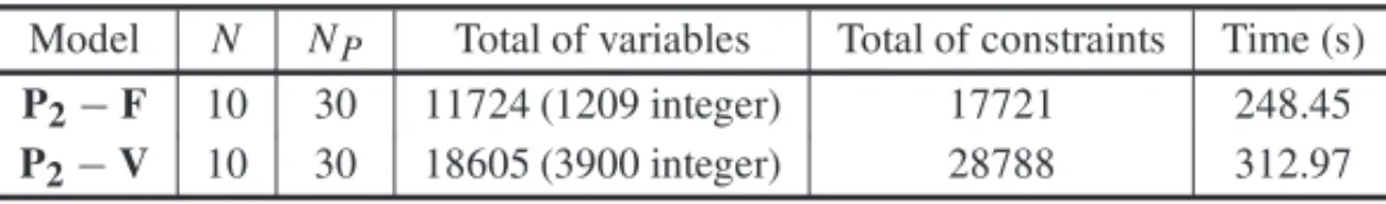
Table 3 describes the experiment withP2−Fand P2−V models in terms of the instance size
of their equivalent deterministic MILP model, and the computational time in terms of CPU time.
Table 3–P2−FandP2−V equivalent deterministic data model.
Model N NP Total of variables Total of constraints Time (s)
P2−F 10 30 11724 (1209 integer) 17721 248.45
P2−V 10 30 18605 (3900 integer) 28788 312.97
Tables 4, 5, 6 and 7 show the comparative results of the modelsP2−FandP2−V with respect
toS0,Si, fi,L B,U B, with precision of 0.1(y=1)for the binary expansion, and to the expect value of the fractions of the unmet demand (shortage fractions) for instances I1, I2 I3 and I4. The first column (column 1− ¯fi) indicates the maximum limit for the expect value of the fraction of unmet demand. The last 3 columns, 1− ¯f1,1− ¯f2and 1− ¯f3, show the service level achieved
for each instance with the experiment, considering a candidate solution with mean values ofS0
andSi, and the mean fraction of unmet demand given by
fim = p,ξ
f(ξ )ip
(NpN)
forP2−V, andS0,Siand fi forP2−F, after 100 runs(M =100), with 30 scenarios(N =30) and 30 periods(NP =30).
Table 4– Comparative numerical results for I1 instance.
P2−Fwith precision 0.1
1-fi S0 S1 S2 S3 f1 f2 f3 LB σLB UB σU B gap lbe lbe 1-f1 1-f2 1-f3
15% 754 56 162 108 0.17 0.51 0.32 153 2.2 151 1.7 1.4 1.4% 1.1% 15.6 15.3 15.5
10% 778 57 163 109 0.17 0.52 0.31 174 1.5 173 2.3 1.5 0.8% 1.3% 10.0 10.1 10.3
5% 805 59 166 112 0.18 0.49 0.33 208 3.0 208 3.0 0. 1.4% 1.4% 5.2 5.0 4.9
1% 839 64 173 119 0.24 0.43 0.33 283 8.6 283 4.3 0.5 3.0% 1.5% 1.2 1.1 1.0
P2−Vwith precision 0.1
1-fi S0 S1 S2 S3 f1m f2m f3m LB σLB UB σU B gap lbe lbe 1-f1 1-f2 1-f3
15% 754 55 162 108 0.14 0.53 0.33 152 1.9 151 1.6 1.09 1.3% 1.1% 15.8 15.3 15.4
10% 778 56 163 109 0.14 0.53 0.33 174 2.9 172 2.1 2.38 1.6% 1.2% 10.9 10.2 10.2
5% 806 58 167 112 0.14 0.53 0.33 209 3.0 210 2.7 0.70 1.4% 1.3% 5.3 4.6 4.8
1% 840 64 173 118 0.15 0.53 0.33 286 7.6 285 2.9 1.0 2.7% 1.0% 1.0 1.1 1.1
Table 5– Comparative numerical results for I2 instance.
P2−Fwith precision 0.1
1-fi S0 S1 S2 S3 f1 f2 f3 LB σLB UB σU B gap lbe ube 1-f1 1-f2 1-f3
15% 738 65 181 120 0.2 0.49 0.31 415 3.0 414 3.8 1.3 0.7% 0.9% 15.2 15.1 15.1
10% 762 65 181 120 0.2 0.49 0.31 474 2.3 472 3.9 2.1 0.5% 0.8% 10.1 10.3 10.3
5% 793 65 179 124 0.2 0.45 0.35 549 4.8 550 3.5 1.7 0.9% 0.6% 4.9 4.8 4.9
1% 829 71 181 126 0.26 0.4 0.34 666 10.8 660 6.4 5.2 1.6% 1.0% 1.1 1.1 1.1
P2−Vwith precision 0.1
1-fi S0 S1 S2 S3 f1m f2m f3m LB σLB UB σU B gap lbe ube 1-f1 1-f2 1-f3
15% 739 60 183 120 0.14 0.53 0.33 418 3.1 417 3.8 0.91 0.7% 0.9% 15.1 15.2 15.1
10% 763 61 182 120 0.14 0.53 0.33 477 2.5 475 3.8 2.44 0.5% 0.8% 9.8 10.3 10.3
5% 794 62 184 122 0.14 0.53 0.33 552 4.9 553 4.4 1.17 0.9% 0.8% 5.0 4.8 4.9
1% 830 67 186 125 0.14 0.53 0.33 671 11.7 666 5.7 5.8 1.7% 0.9% 1.0 1.1 1.1
Table 6– Comparative numerical results for I3 instance.
P2−Fwith precision 0.1
S0 S1 S2 S3 f1 f2 f3 LB σLB UB σU B gap lbe ube 1-f1 1-f2 1-f3
785.7 55.2 164.3 112.0 0.22 0.58 0.19 179.9 2.8 183.2 2.2 3.3 1.6% 1.2% 13.7 9.1 4.7
P2−Vwith precision 0.1
S0 S1 S2 S3 f1m f2m f3m LB σLB UB σU B gap lbe ube 1-f1 1-f2 1-f3
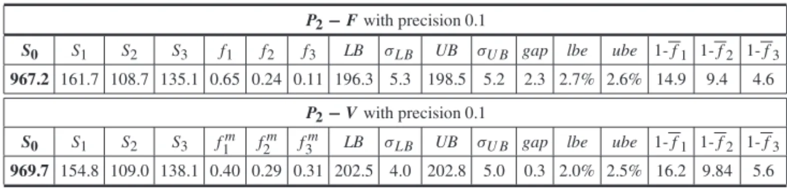
Table 7– Comparative numerical results for I4 instance.
P2−Fwith precision 0.1
S0 S1 S2 S3 f1 f2 f3 LB σLB UB σU B gap lbe ube 1-f1 1-f2 1-f3
967.2 161.7 108.7 135.1 0.65 0.24 0.11 196.3 5.3 198.5 5.2 2.3 2.7% 2.6% 14.9 9.4 4.6
P2−Vwith precision 0.1
S0 S1 S2 S3 f1m f2m f3m LB σLB UB σU B gap lbe ube 1-f1 1-f2 1-f3
969.7 154.8 109.0 138.1 0.40 0.29 0.31 202.5 4.0 202.8 5.0 0.3 2.0% 2.5% 16.2 9.84 5.6
rule. Also, from Tables 4 and 5, we verify thatS0values decrease and Si values increase ash0p increases forP2−F, as well as forP2−V. Table 6 shows that the results forP2−V model are
associated with a smaller gap. From Table 7 we verify that both rationing rules are similar even considering a non-stationary stochastic process to generate the demands.
The results suggest in general that the configuration of the experiment, taking 10 runs for the estimation of the lower bound, is reasonable, since the gap and the standard deviation are small. We observe that the percentage errorslbeandubeare close to 1% for the instances I1 (except, when 1− ¯fi =1%) I2 and I3, and between 2% and 3% in the other cases.
6 CONCLUSION
Based on stochastic programming, this research proposed a new comprehensive approach re-garding the representation of demand uncertainty in the problem of determining the optimal parameters of an inventory control system of a single item with periodic review and assessment of shortage in an arborescent two-echelon logistics network over a finite time horizon. Indeed, this approach allows the relaxation of assumptions on the behavior of uncertain parameters, and in particular on the stochasticity behavior of the demand for the item. In relation to shortages of the item that may occur, we introduce a variable rationing rule at the DC that deals with imbal-ances and indirectly improves the service levels. Specifically, we proposed mixed-integer linear programming models that are deterministic equivalent formulations of the proposed two-stage stochastic programming models to obtain optimal review interval and target level of the control system(R,S)of a logistics network with a DC and many retailers. To obtain approximate solu-tions for the deterministic models, we used a sampling technique to generate finite scenarios with discrete values for demand levels. Both stationary and non-stationary processes were considered to represent the uncertain demand.