*e-mail: [email protected]
Numerical Modeling of Welded Joints by the
“Friction Stir Welding” Process
Diego H. Santiagoa, Guillermo Lomberaa*, Santiago Urquizaa, Anibal Cassanellia, Luis A. de Vediab
aFacultad de Ingeniería, Univ. Nac. de Mar del Plata,
J.B. Justo 4302, 7600, Mar del Plata, Bs. As., Argentine
bITPJS, Univ. Nac. De San Martín - CNEA, CIC, San Martín , Bs. As.,Argentine
Received: March 17, 2004; Revised: September 28, 2004
The present work is aimed to simulate the Friction Stir Welding process as a three-dimen-sional thermally coupled viscoplastic flow. A Finite Element technique is employed, within the context of a general purpose FEM framework, to provide the temperature distributions and the patterns of plastic flow for the material involved in the welded joints. The computational tool presented here may be of great relevance for technologist seeking to set the process control vari-ables, as they are intended to obtain suitable material properties that yield the adequate on service response of the structural components.
Keywords:Friction stir welding (FSW), viscoplastic modeling, three-dimensional modeling, finite elements model, aluminum butt welding
1. Introduction
Welding by means of the friction stir welding (FSW) process is a technique for joining two sheets or thick plates with only mechanic energy as input. In Fig. 1 we observe a schematic representation of the FSW process, the tool con-sists essentially in a rotating solid cylinder with a protrud-ing screwed insert of smaller diameter (Fig. 2). The main cylinder prevents the material from being expulsed from the pieces to be welded thus preventing the formation of voids or other defects in the welded zone.
Once the pieces to be welded are presented and firmly restrained on the welding fixture, the protruding insert of the tool is forced within the pieces to be welded until the cylindrical part is in contact with the work surface. As the tool rotates and progresses along the seam, the friction heated and softened material flows around the insert towards its trailing part where it consolidates to create a solid phase high quality weld. Notice that the tool axis has typically a tilt of some degrees (2° or 3°) with respect to the vertical, in order to facilitate the weld nugget formation.
Several papers have been written on the FSW process, Flores et al.1, Murr et al.2, Liu et al.3 and Midling about the microstructural aspects of the welded aluminum alloys and also the works of Dawes and Thomas4,5 who described the FSW process summarizing its advantages and
disadvan-tages. However, although considerable experimental pub-lished works have been reported, there are relatively few papers about modeling the FSW process. Gould et al.6 de-veloped an analytical heat flow model for FSW. The model is based on the well known Rosenthal equation7, which de-scribes a stationary temperature field in a semi-infinite plate due to a mobile heat source. A lot of simplifications had to be introduced in order to obtain a closed solution in the tem-peratures field. Stewart et al.8 used an approximate energy balance to predict the weld shape and the temperatures in-side the welded zone. The temperatures field was also pre-dicted using the method developed in the reference 7. It should be stressed that because of the problem characteristics, where the plastic deformations are dominant, good results can be expected using thermomechanically coupled viscoplastic flow models9,10. In addition, due the cinematic and geometric char-acteristics of the process, the problem turns out to be three-dimensional, which together with the existence of strong gra-dients in the deformation velocities around the insert, im-poses a high computational demand. Recently9, scientists have entered upon this type of modeling but with some kind of limitations considering the localized densification possi-bilities, among other questions.
lead-ing element when predictlead-ing the microstructural properties in the affected zone and when optimum design or improve-ment of the welding tools geometry are needed.
In virtue of the complex physics involved during the FSW process, the aim of the present research is to improve the process comprehension by means of numerical
Figure 2. Tetrahedral finite element and tool sketch.
modeling, inquiring into the basic aspects of the process so as to determine the computational exigency level that this type of modeling requires for the adequate representation of the principal phenomena involved, towards a further sen-sibility analysis.
2. Fundamental Equations
2.1. Mechanical model
Leaving aside the inertial and volume forces, the equi-librium equations in a volume Ω of material with a ∂Ω boundary, can be written in the following way10:
(1)
where σ is the Cauchy stress tensor.
The deformation rate vector is related to the symmetric part of the velocities field gradient according to:
(2)
Assuming the material as incompressible, the continu-ity equation must be satisfied for the whole dominion Ω:
(3)
If we adopt a flow formulation for modeling the large plastic deformations involved in the stir-welding process, the stress deviator tensor S can be related to deformation rate tensor D – which is actually a deviator in virtue of the incompressibility – by the following relation:
(4)
where µ is the effective viscosity of the material and p the hydro-static pressure. Besides, σe is the effective stress or the second stress invariant and εe is the effective deformation rate or the second in-variant of the deformation rate.
In this work it was assumed a rigid and viscoplastic material where the flow stress depends on deformation rate and temperature. This is represented by the following rela-tion11:
, (5)
where α, Q, A and n are material constants, R is the ideal gas con-stant and T is the absolute temperature.
The material constants can be determined using stand-ard compression tests. The mechanical model is completed after describing the appropriate boundary conditions.
2.2. Thermal model
The temperatures distribution is obtained by solving the heat balance equation10:
(6)
where ρ is density, Cp the heat capacity, k the thermal conductiv-ity, θ the temperature and γthe inner rate of heat generation by dissipation of viscoplastic power.
It is assumed that about 90% of the plastic power is trans-formed into heat. The term corresponding to the heat gen-eration rate by mechanical work can be expressed as the contracted product of stress with deformation rate, as fol-lows:
γ = η S:D (7)
where η is the power fraction which is not absorbed by micro-structural defects.
Properties of pure aluminum where adopted for the me-chanical parameters as well as for the temperature depend-ent conductivity and specific heat.
2.3. Geometric model
In the present study it is assumed a reference frame-work fixed to the welding tool, in such a way that the plate moves towards it with a fixed velocity (1.05 mm/sec) and with an initial temperature (25 °C) both imposed in the lead-ing surface of the zone to be studied.
Since the tool insert surface is mechanized with a heli-cal shape, the effect of running down flow produced for such geometry is simulated imposing a running down ve-locity component at the insert surface. This veve-locity is a function of the advancing speed of the insert (1.067 mm/ revolution) and of the rotation rate of the tool (11.7 revolu-tions/sec)
Material data and other parameters from the model are included in the Tables 1 to 3.
2.4. Numerical modeling
The base plate was modeled with a finite tetrahedral el-ement netting of the Taylor-Hood type10, that is tetrahedrons P2-P1, with quadratic interpolations for velocities and lin-eal interpolations for stresses, so as to get stability from stresses interpolations for the null divergence condition to-gether with an appropriate capture of the stress gradients in boundary layers. The netting used had approximately 10200 elements with 15500 velocity nodes (Fig. 2).
The resolution algorithm consists of two steps: in the first one the velocities field is obtained assuming a fixed temperatures field. There is an iteration made by successive replacements in order to produce a non-linear adaptation of the viscosity values according to deformation rates obtained in the previous iteration. The discrete equations are obtained from the classical formulation of the Stokes problem for totally incompressible viscous flow and according to the interpolations above mentioned, adding the artificial pseudo-compressibility of Chorin12. The linear equations system for each iteration is solved by the conjugated square gradients with a preconditioner of incomplete factorization of type LU according to the scheme proposed by Y Saad and Sparse13. In the second step the temperatures field is solved with quadratic interpolation as a problem of convection-diffusion assuming the velocities field obtained in the first step. The numerical solving method is the same as in the first step.
Although the stationary solution is required, an advance-through-time scheme totally implicit was used fundamen-tally as a preconditioner of the equations system.
4. Results
4.1. Velocities field
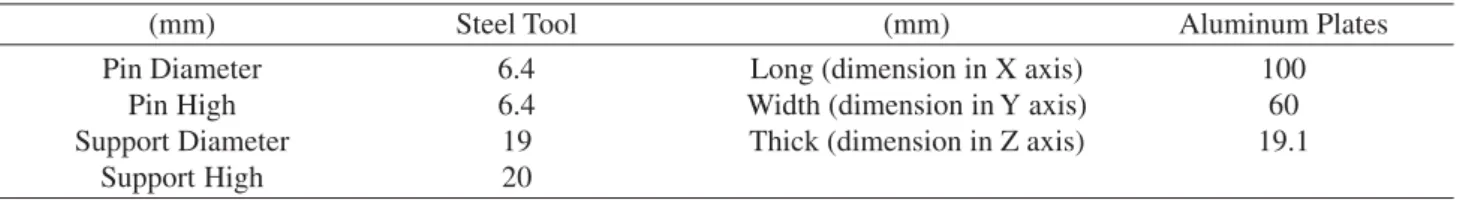
In the results no tool graphic is shown in order to make easier the visualization of data in Figs. 3, 4 and 5.
Figure 3 shows flow lines of the material in the insert region of the tool. It is clearly observed the running-down effect that produces the grooving of the surface. It is also
Table 1. Thermal Property.
Property Steel Tool Aluminum Plates ρ [Kg/m3] 7.8 103 2.7 103 Cp [J/Kg °C] 0.5 103 1.05 103
k [W/m °C] 40.0 207.0
Table 2. Dimensions of the tool and the aluminum plate.
(mm) Steel Tool (mm) Aluminum Plates
Pin Diameter 6.4 Long (dimension in X axis) 100
Pin High 6.4 Width (dimension in Y axis) 60
Support Diameter 19 Thick (dimension in Z axis) 19.1
Support High 20
Table 3. Viscosity Law Parameters.
Material A α (mm2 N-1) n H (J mol-1)
seen how the material stays close to the insert surface dur-ing several rotations of the tool before followdur-ing its course in the welding direction.
Figure 4 shows the velocity module in planes XZ and YZ that go through the center of the tool insert. It can be observed a strong boundary layer in the insert surface.
4.2. Temperatures field
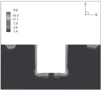
The temperatures field and material velocities are shown in Fig. 5. It is clearly observed that the heat is concentrated at the insert surface, where the largest deformation rates are produced, and as a consequence, the greatest heat genera-tion.
Figure 6 shows sections in planes XZ and YZ
respec-tively, from temperatures field of the above figure. In plane XZ is observed the convective dragging effect on the peratures field produced by the welding speed. In the tem-peratures field showed in plane YZ is observed a higher temperature in the right side of the insert, as in this side the tangent velocity direction in the insert opposes to the weld-ing velocity direction. In Fig. 7 experimental results are com-pared to those obtained in the simulation. The abscises axis are the tool position in the welding direction, were zero position is the tool center. This data is taken 12.7 mm from the interface between plates. The experimental data is ob-tained from the reference 9.
5. Conclusions
Figure 3. Flow lines of the material in the insert region of the tool.
Figure 5. Material velocities and temperatures field respectively.
Figure 6. Temperatures field in planes XZ and YZ respectively.
Figure 7. Experimental results compared to obtained in the simu-lation.
A computational three-dimensional finite element model of the FSW process was presented so as to describe the main aspects of the process and to show and evaluate the compu-tational requirements needed for the appropriate capture of the main phenomena involved. The results obtained are fit-ting with those reviewed in literature. The presence of very strong gradients in the velocities field in the surroundings of the tool insert were found which requires a re-evaluation of the densifications used in such areas and towards further sensibility analysis so as to obtain nets optimally suited with the problem requirements and optimized from the compu-tational cost point of view.
1. Flores, O.V.; Kennedy, C.; Murr, L.E.; Brown, D.; Pappu, S.; Nowak, B.M.; McClure, J. Microstructural issues in a friction-stir welded aluminum alloy, Scr. Mater, v. 38, p. 703, 1998.
2. Murr, L.E.; Liu, G.; McClure, J.C. A TEM study of pre-cipitation and related microstructures in friction-stir-welded 6061 aluminum, J. Mater. Sci., v. 33, p. 1243, 1998.
3. Liu, G.; Murr, L.E.; Niou, C.S.; McClure, J.C.; Vega, F.R. Micro- structural aspects of the friction-stir welding of 6061-T6 aluminum alloy, Scr. Mater, v. 37, p. 335, 1997. 4. Dawes, C.J.; Thomas, W.M. Friction stir process for
aluminum alloys, Welding J. v. 75, p. 41, 1996. 5. Dawes, C.J. An introduction to friction stir welding butt
welding and its developments, Welding and Fabrica-tion Jan, 1995.
6. Gould, J.E.; Feng, Z. Heat flow model for friction stir welding of aluminum alloys, Journal of Material Processing and Manufacturing Science 7, 1998. 7. Rosenthal, D.; Schemerber, R. Thermal study of arc
weld-ing, Welding J., v. 17, 208s, 1938.
8. Stewart, M.B.; Adams, G.P.; Nunes, A.C.; Romine, P. A combined experimental and analytical modeling ap-proach to understanding friction stir-welding, Devel-opments in Theoretical and Applied Mechaninics, SECTAM XIX, p. 472, 1998,
9. P. Ulysse. Three-dimensional modeling of the friction stir-welding process International Journal of Machine Tools and Manufacture, v. 42, p. 1549-1557, 2002. 10. Zienkiewicz, O.C.; Taylor, R.L. (Eds.), The Finite
Ele-ment Method, fourth ed., McGraw-Hill, UK, p. 2, 1991. 11. Sheppard, T.; Wright, D.S. Determination of flow stress: Part 1 constitutive equation for aluminum alloys at el-evated temperatures, Metals Technology, June, p. 215, 1979.
12. Chorin A.J. Math. Comp, v. 22, p. 745-762, 1968. 13. Saad Yuocef, SPARSEKIT: a basic tool kit for sparse