(Recebido em 05/10/2008; Texto Final em 11/07/2009).
(Modelagem 3D do Fluxo de Material e da Temperatura na Soldagem “Friction Stir”)
Diego Santiago1, Santiago Urquiza1, Guillermo Lombera1, Luis de Vedia2
1Dto.de Ing. Mecánica, Univ. Nac. de Mar del Plata (CONICET), 7600 Mar del Plata, Buenos Aires, Argentina.
dsantiago@fi.mdp.edu.ar, glombera@fi.mdp.edu.ar, santiagourquiza@fi.mdp.edu.ar 2 Instituto Sabato (UNSAM-CNEA), CIC, 1650 San Martín, Buenos Aires, Argentina
ldevedia@cnea.gov.ar
Abstract
The process of Friction Stir Welding (FSW) is a welding method developed by the “The Welding Institute” (TWI) of England in 1991. The welding equipment consists of a tool that rotates and progresses along the joint of two restrained sheets. The joint is produced by frictional heating which causes the softening of both components into a viscous-plastic condition and also by the resultant flow between the sheets to be joined. Numerical Modeling of the process can provide realistic prediction of the main variables of the process, reducing the number of experimental tests, thus accelerating the design processes while reducing costs and optimizing the involved technological variables. In this study the friction stir welding process is modeled using a general purpose finite element based program, reproducing the material thermal map and the corresponding mass flow. Numerical thermal results are compared against experimental thermographic maps and numerical material flow results are compared with material flow visualization techniques, with acceptable concordance.
Key-words:Friction stir welding (FSW); Three-dimensional modeling; flow; temperature, finite element.
Resumo: O processo denominado “Friction Stir Welding” (FSW) é um método de soldagem desenvolvido pelo “The Welding Institute” (TWI) na Inglaterra em 1991. O equipamento de soldagem consiste de uma ferramenta que gira e avança ao longo da interface entre duas chapas fixas. A junção é produzida pelo calor gerado por fricção o qual causa o amolecimento de ambos os componentes atingindo uma condição visco-plástica e também pelo escoamento resultante entre as laminas a ser unidas. A modelagem numérica do processo pode fornecer uma predição real das principais variáveis do processo, reduzindo o número de testes experimentais, acelerando, portanto os processos de projeto ao mesmo tempo em que reduz custos e permite a otimização das variáveis tecnológicas envolvidas. Neste trabalho, o processo de soldagem por fricção é modelado empregando um programa de propósito geral baseado no método dos elementos finitos, procurando reproduzir a distribuição térmica e o correspondente escoamento de massa. Os resultados numéricos térmicos são comparados com distribuições termográficas experimentais e os resultados numéricos de escoamento de massa são comparados com aqueles obtidos a partir de técnicas experimentais de visualização, atingindo uma concordância aceitável.
Palavras-chave:Friction stir welding (FSW); Modelagem 3D; escoamento; temperatura, elementos finitos.
1. Introduction
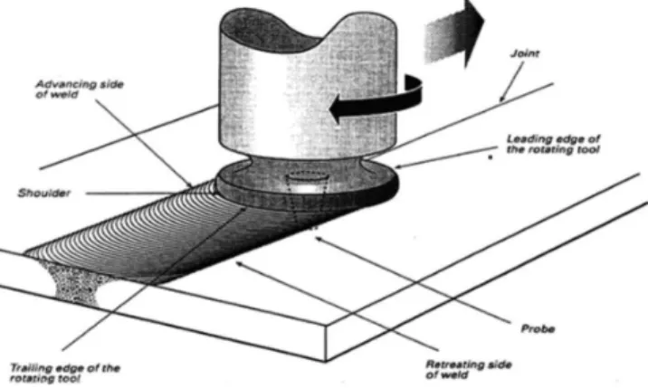
The Stir-Welding or Friction Stir Welding (FSW) [1] is a technique that involves the joining of two thick sheets or plates using mechanical means. Figure 1 shows a schematic representation of the FSW process, the tool consists of a shoulder, normal to the axis of rotation of the tool and a small diameter probe connected to it.The tool shoulder, with larger diameter than that of the probe, prevents the material from being expelled fromtheworkpiecetobewelded.Thisminimizestheformation ofvoidsintheweldedarea.Ontheotherhand,themainpart of process heat input is induced by friction between shoulder
tool and plates. Usually the probe is “threaded” to increase the generation of frictional heating and a greater mixing effect on the materials.
Once the sheets or plates are butted on a common axis, the rotating tool is plunged into the welding workpiece until the shoulder is brought into close contact with the two parts to bejoined.Oncetheprobeisinserted,itmovesinthewelding direction. As the tool moves along the joint line, the heated and plasticizedmaterialissweptaroundtheprobetotherearwhere itconsolidatesandformstheweld.Itresultsinasolid-statehigh qualityweld.Noticethatthetoolaxisistypicallytiltedbyseveral degrees(2ºor3º)fromtheverticaltofacilitateconsolidationof theweld.
alloy welding, and those written by Dawes andThomas [5,6] describing the FSW process, summarizing its advantages and disadvantages.Thereareseveralworksonnumericalsimulation in relation with this process. Gould et al [7] developed an analytical heat transfer model for FSW. The model is based on thewellknownRosenthalequation[8]whichdescribesaquasi stationary temperature ield over a semi-ininite plate due to a moving heat source. Kovacevic et al [9,10] carried out thermal and thermo-mechanical analyses using inite elements. These analyses are based on a heat source model, not considering the thermo-mechanical coupling generated by plastic low. It is worthmentioningthatduetothecharacteristicsofthisproblem, by using fully coupled thermal-mechanical viscoplastic low models [11-13], good results can be expected where plastic deformations commonly occur. Besides, due to its geometric and kinematic characteristics, the problem is mainly three-dimensional, which together with the presence of high strain rate gradients around the probe imposes a high computational demand. In this sense, this kind of modeling was tackled by Colegroveetal[13].usingthe“CFDpackageFLUENT”,where a coupled thermomechanical viscoplastic model for aluminum materialwassolvedobtaininggoodresultsasregardsmaterial lowdistribution.Recently,Nandanetal[14,15]reportedresults of stainless steel FSW simulation by using this kind of models withgoodagreementbetweencomputedtemperatureieldand experimental data, showing the versatility of the viscoplastic lowmodelstorepresentlargedeformationprocessesasinFSW. Nevertheless, none of the previously quoted papers contrast materiallowsimulationwithexperimentaldata.
Figure 1. Friction Stir Welding (FSW) schematic process.
In this work, coupled modeling of material low and temperatureielddistributionwascarriedoutforasteadystate problem. The thermal model boundary conditions considered the convection heat loss and heat transfer through the tool and the base plate. Heat generation through viscous dissipation wasalsotakenintoaccount.Resultsobtainedwerecontrasted with experimental data. Thermal results were compared with experimental data obtained by thermographic imaging. The modeled low structure around the tool was analyzed comparing results with those existing in previously published worksofexperimentalresearchers[2-4]andalsowithourown data coming from photographic imaging corresponding to the
contact surfaces of the joint, more speciically, in the vicinity of theleadingzonewerethejointwasnotyetfullachieved.This technique allows to qualitatively asses the experimental low patterns around the tool, avoiding the implementation of more sophisticated (e.g., particle tracing) techniques and facilitating the validation of these aspects of the numerical results.
2. Governing equations 2.1. Mechanical model
Neglecting inertial and volume forces, the equilibrium equation in a volume of material Ωwithboundary∂Ω can be writtenas[16]:
Ω
=
⋅
∇
σ
0
in
(1) whereσ
is the Cauchy stress tensor . Tractions Tºi can beprescribed in a part of the boundary ∂Ωt(Neumann conditions), whilethevelocitycomponentsuºi can be speciied in the rest of the surface ∂Ωu (Dirichlet conditions).This can be expressed as follows:
( )
NDim
i
º
u
e
NDim
i
º
T
e
u i i i ti i i,..,
1
,
in
,..,
1
,
in
=
Ω
∂
=
⋅
=
Ω
∂
=
⋅
u
n
σ
(2)where∂Ω = ∂Ωt ∂Ωuy ∂Ωt∩ ∂Ωu = ∅, n istheunitoutward normal to the contour ∂Ω, ei is the unit basis vector for a three-dimensional Cartesian coordinate system and u is the velocity vector. The deformation rate vector is related to the symmetric part of the gradient of the velocity ield according to
(
)
2
Tu
u
D
=
∇
+
∇
(3)Assumingthematerialisincompressible,thenthefollowing continuum equation must be fully observed on Ω
(4)
If a low formulation for modeling the large plastic deformations involved in the stir-welding process is adopted, the stress tensor deviator S can be related to the deformation rate tensor D –which actually is a deviator by virtue of the incompressibilityhypothesis–asgivenby:
e
e
2
-3
p
µ
σ
σ
µ
ε
=
=
=
S
D, S
I
(5)
D
D
S
S
:
3
2
:
2
3
2 e 2 e
=
=
ε
σ
(6)Thisworkassumesaviscoplasticconstitutivemodelwhere stresses depend on deformation rate and temperature. This is represented by [17]:
(7)
whereα, Q, A and n are material constants, R is the gas constant and T is the absolute temperature. Material constants can be determined using standard compression tests. The mechanical model is completed after describing the appropriate boundary conditions.
2.2. Thermal Model
Temperature distribution is determined by solving the heat balance equation [16]:
(8)
whereρ is the density, Cp is the heat capacity, k the thermal conductivity, θ the temperature and γ the internal heat generation rate due to viscoplastic power dissipation. It is assumed that 90%oftheplasticpowerconvertstoheat[18].Thetermthat corresponds to the rate of heat generation through mechanical work can be expressed as the product between stress and deformationrate,asfollows:
D
S
:
η
γ =
(9)withηthefractionofpowernotabsorbedinmicrostructural defects.
Properties of pure aluminum were adopted, both for the mechanicalparametersaswellasforthetemperature-dependent conductivity and speciic heat. A thermal low qº can be prescribed on a part of the boundary ∂Ωq,whilethetemperature
θ º can be speciied in the rest of the surface∂Ωθ. This can be writtenas:
(10)
Where ∂Ω = ∂Ωq∪ ∂Ωθ and n istheunitoutwardnormal to the boundary ∂Ω. The contribution qº is due to the cooling of the surfaces by convection and also by the heat transmission through the contact interfaces, e.g., the “tool-plates” and the “base-plates” interfaces.
2.3. Geometric Model
In this work, it is assumed a reference frame ixed to the weldingtool,sothattheplatemovestowardsthetoolataspeed (V = 2.0 mm/s) and temperatures ( a = in=25ºC)imposedon
the entrance surface of the region under study. All boundary conditions are detailed in Appendix A
The surface of the tool probe is spirally threaded. The effect of the ascending low produced by such spiral is simulated imposinganupwardvelocitycomponentontheprobesurface. This velocity is a function of the spiral step (Pitch=1,2 mm/rev) and the tool rotation velocity ( = 22,5 rev/s)
Data for the materials properties [19] and the constitutive law constants [17] of the model are shown in tables 1 and 2, respectively.
Table 1. Thermal properties for the tool (steel), the base (steel) and the aluminum plates.
Properties
iedades ρ [Kg/m
3] Cp[J/KgºC] k[W/mºC]
Aluminum 2.7 103 1.05 103 207.0
Steel 7.0 103 0.5 103 40.0
Table2.ViscosityLawparameters.
Material A α [mm2 N-1] N H [J mol-1]
Alloys 1S 0.224 1013 0.052 4.54 177876.4
Alsoitisadoptedthatthematerialincontactwiththetool has a 50 % relative slipping(C=0.5) as suggested by Ulysse [11], which produce realistic results and simpliies the model implementation.Figure2showsaperspectiveofthegeometry of the problem and the dimensions used. The dimensions are basedonaworkofCabotetal[19].
Figure3showsthedifferentareasoftheproblem.Area1 representsthesteelbasewheretheplatestobeweldedareplaced and Area 4 corresponds to the tool. Areas 2 and 3 represent the plates to be welded, which have been meshed with low and high concentration of elements, respectively. Figures 4a and 4b showtheassembledgeometry.Figures4cand4dshowthemesh details of densiied regions corresponding to Areas 2 and 3.
3. Numerical model
ThebaseplatewasmodeledusingaTaylor-Hoodtetrahedron [16]initeelementmesh,i.e,P2-P1tetrahedronelementswith quadratic interpolation for velocity ield and linear for pressure, whicharediv-stable[20]andalsoallowsanadequatecapture of the high tension gradients present in the neighborhood of the tool. The implemented mesh had approximately 85000 elements with 107000 velocity nodes (Figure 4). This case was solved using the general proposed solver code (Solver GP) developed by Urquiza et al [21,22].
Thesolutionalgorithmconsistsoftwosubsteps:theirstone
Figure 3. Geometry decomposition.
Figure 4. Perspective of model mesh (a) and details of densiied zones (b, c and d).
with quadratic interpolation derived from the corresponding advection-diffusion problem and assuming ixed the velocity ield as provided by the irst sub-step. The solution of the algebraic system is the same as in the irst substep.
Even though a stationary solution is required, an implicit time advancement scheme was implemented, mainly used as preconditioner for the equation systems.
4. Results
4.1. Temperature fields
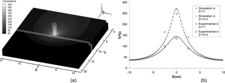
The temperature values obtained in the modeling were contrasted against experimental data measured by thermograph.
The infrared thermal camera used is a Fluke Ti30, the images generated are 120x160 pixel size and contain a temperature measure for each pixel. The precision of the temperature measurement of this camera is ±2% at full scale. Thermograph datacorrespondtoaweldmadewiththesameprocessparameters usedinthiswork.ThosedatawereobtainedatCAC-CNEA.
Comparisons between model prediction and experimental dataareshowninFigure5b.Thisgraphictakesthetemperature valuesofthetopsurfaceoftheplatesintwocrosswelddirection lines placed at 10mm and 14.4mm ahead of the tool rotation axis (seethewhitelinesinFigure5a).Itcanbeobservedareasonably well agreement between temperature values obtained with the modelandwiththosecomingfromexperimentaldata.
Figure5.Comparisonbetweenthedatacorrespondingtothethermographicimageandthoseobtainedbysimulation.
Figure 6. Section of the temperature ields in the planes XY (a) and YZ (b) in the centre of the tool.
Figures 6a and 6b show the temperature distributions at the tool’s rotation center (see igure 2) on XY and YZ planes respectively.Also, igure 6a depicts the contact zone between the tool and the plates. As can be observed, the temperature is
6b illustrates the convective drag effect over the temperature ieldproducedbytheweldvelocity.
As it is depicted in igures 5 and 6, the resulting temperature distribution in the tool is practically linear in a direction coincident withtherotationaxis.Therefore,thetoolmeshmaybereplaced by a Neumann condition on the Tool-Plates interface, reducing the computational cost of the problem.
4.2. Velocity fields and material flow
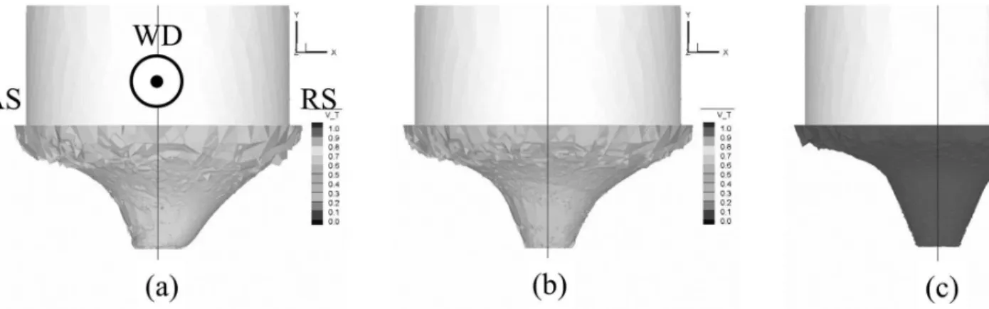
Figure 7 shows the Iso-surfaces of the velocity module corresponding to 3 mm/s (igure 7a), to 5 mm/s (igure 7b) and to20mm/s(igure7c).Thoseiguresillustratesthatzoneswith velocitiesclosertotheweldvelocity(Vw=2mm/s)aregreater in size for the retreating side than for the advancing side. This isinagreementwiththeexperimentalworkcarriedoutbyMurr [3], where it is reported a thermo-mechanically affected zone aroundtheprobewhichisatleasttwiceaslargeontheretreating sidecomparedwiththatfortheadvancingside.
In igure 7c the velocity iso-surface corresponds to values ten timesgreaterthantheweldvelocity.Inthiscasethedelimited
zone is almost symmetrical. Therefore, it can be said that it represents approximately the boundary between the Thermo-Mechanically Affected Zone (TMAZ) and the Stir Zone (SZ) subjected to plasticization and agitation. This is in accordance withthatreportedbyGuerraetal[25].Inthisway,itwillbe possible to predict different microstrucutral regions (TMAZ, SZ) whoseinturndeterminestheinalpropertiesoftheweldedjoint. Consequently, this computational model has the potentiality to optimize the properties of the joints as a function of the different size of the microstructural regions occurring around the tool. This isanimportantaspectwheremodelingtoolscancontributeto improvetheweldedjointsviaabettercontrolofthedistribution of inal material properties.
Figure8showsthepathofthestreamlinesaroundthetool. The low lines of this igure represent the paths of material particles that go through the affected zones in the neighborhood ofthetooltip.BeingtheadvancingdirectionWDcoincidentwith the positive Z axis (+Z), the pathlines advance in the negative directionofthataxis(-Z).Theinitialpositionofthelowline showninigure8acorrespondtothejointposition(x=0)at3mm ofthebottomplates(y=3mm).Thisflowlineclearlyshowsthe
Figure 7. Iso-surfaces of 3 mm/s (a), 5 mm/s (b) and 20 mm/s (c) velocities.
ascending effect produced by the threaded surface of the pin. Fromthesameigureitcanbeobservedthatoncethelowline reaches the top surface, contacting the tool shoulder, it takes a descending path rotating several times before continuing its course. As a consequence, the material stays close to the surface of the tool pin remaining inside to the SZ (velocity module>20mm/ seg)duringseveralrevolutions.Thistypeoflowpatternswas observedbyGuerraetal[25].There,wasrecognizeda“rotational zone”equivalenttoSZ,wherethematerial“ismovedbyentering onto the rotational zone, undergoing several revolutions, and inallydroppingoffinthewakeofthenib”.
Figure8bshowsanarrangementoflowlinescomingfrom thejointposition(x=0)alongthewholethicknessoftheplates (0mm<y<6.25mm). It can be seen how the low lines coming fromthelowerhalfoftheplatesentertotheSZ,whiletheothers circumvent the SZ, going through the TMAZ before escaping from that zone on straight path along the welding direction. Also, it can be observed how the low lines coming from the upperhalfoftheplatearedrivenbytheinteractionwiththetool pinwhilethosecomingfromthelowerhalfaredrivenbythe interactionwiththetoolshoulder.
To compare the material low obtained in the modeling with experimental results [19], the deformations produced in the material located in front of the tool were observed. In this zone the material of the surfaces to be joined has become greatly deformed but still remains unwelded. In this way it is possible to visualize the low patterns without using particle tracers. Figure 9 illustrates these facts comparing pictures of the material located on the leading side (LS) of the tool with the corresponding surfaces generated by the modeled material lowlines.Itisobservedthatthemodeledplasticallydeformed zone (igure 9d) is larger than the one obtained experimentally (igure 9c), mainly around the tool shoulder. This difference can be attributed to the fact of applying a uniform relative slipping conditiontothewholesurfaceofthetool.Thus,itcanbeinferred that the velocities applied to the tool shoulder in the model are higher than the ones observed experimentally, generating a greater deformation zone. Also, from the results observed in igure 9d, can be estimated the thickness of the deformed zone in a direction perpendicular to the shoulder surface. As was stated by Kumar et al [26] the relative size of the deformed zones drivenbytheshouldermovementwithrespecttothosedrivenby thepinaredeterminantforwellbehavedjoints.
5. Conclusions
A three-dimensional computational model was presented through Finite Element modeling of the FSW process. The results are congruent with those observed experimentally, reproducing realistically the main characteristics of the low patterns prevailing in the neighborhood of the tool.
With the low line analysis were recognized two speciic zoneswherethematerialundergoesdifferentpatternsoflow. Itisnoticeablethepresenceofaregionadjacenttothewelding probe with very strong gradients in the velocity ield, and anotherzone,surroundingtheformer,wherethelowvelocities are considerably lower. Consequently, the material passing throughoneofthesezoneswillbesubjectedtoaverydifferent thermomechanical history than the material going through the other. This in turn will inluence in a distinctive manner the microstructural characteristics of the welded material in each region. As a result, the developed model has the potentiality to identifydifferentprocesszoneswhichcanbehelpfultopredict and optimize the main process parameters of FSW. In this sense, this kind of computational models can contribute to reduce labors on designing and setting experimental trials.
Futureeffortsmustbeorientedtowardimprovingthecontact conditions on the interfaces where the material become in contactwiththetooltipandtheshoulder,inordertoattainbetter adjustment of the volumes of material driven by the tool.
6. Acknowledgments
We are grateful to Pedro Cabot and Alberto Moglioni of CAC-CNEA for their advice and technical support on setting the experimentalmeasurementemployedinthiswork.
7. References
[1]THOMAS,M.W.etal.,FrictionStirButtwelding.GBPatent Application No.9125978.8 Dec 1991. US Patent No.5460317, Oct. 1995.
[2] FLORES, O.V. et al., Microstructural issues in a friction-stir weldedaluminumalloy,Scr.Mater.,v.38,p.703,1998.
[3] MURR, L.E.; LIU, G.; McCLURE, J.C.A TEM study of precipitationandrelatedmicrostructuresinfriction-stir-welded 6061 aluminum, J. Mater. Sci., v.33, p.1243, 1998.
[4] LIU, G. Et al, Micro- structural aspects of the friction-stir welding of 6061-T6 aluminum alloy, Scr. Mater., v.37, p.335, 1997.
[5] DAWES, C. J.; THOMAS, W.M. Friction stir process for aluminum alloys, Welding Journal, v.75, p.41, 1996.
[6]DAWES,C.J.Anintroductiontofrictionstirweldingbutt welding and its developments, Welding and Fabrication, Jan. 1995.
[7]GOULD,J.E.;FENG,Z.Heatlowmodelforfrictionstir welding of aluminum alloys, J. Mater. Process. Manu., v.7, 1998.
[8] ROSENTHAL, D.; SCHRMERBER, R. Thermal study of arcwelding,WeldingJournal,v.17,p.208,1938.
[9]CHEN,C.M.;KOVACEVIC,R.Finiteelementmodelingof
frictionstirwelding–thermalandthermomechanicalanalysis, Int. J. Mach. Tool. Manu., v.43, p.1319-1326, 2003.
[10]SONG,M.;KOVACEVIC,R.Thermalmodelingoffriction stirweldinginamovingcoordinatesystemanditsvalidation, Int. J. Mach. Tool. Manu., v.43, p.605-615, 2003.
[11] ULYSSE, P. Three-dimensional modeling of the friction stir-welding process, Int. J. Mach.Tool. Manu., v.42, p.1549-1557, 2002.
[12]SANTIAGO,D.etal.,Numericalmodelingofjointswelded by“frictionstirwelding”process,Materials Research, v.7, n.4, p.569-574, 2004.
[13] COLEGROVE, P.A.; SHERCLIF, H. R. 3-Dimensional CDF modelling of low round a threated friction stir welding tool proile, J. Mater. Process. Tech., v.169, p.320-327, 2005. [14] NANDAN,R.etal,Numericalmodellingof3Dplasticlow andheattransferduringfrictionstirweldingofstainlesssteel, Science and Technology of Welding and Joining, v.11, p.526-537, 2006.
[15] NANDAN, R. et al, Three-dimensional heat and material lowduringfrictionstirweldingofmildsteel,ActaMaterialia, v.55,p.883–895,2007.
[16]ZIENKIEWITZ,O.C.;TAYLOR,R.L.Theiniteelement method.McGrawHill,v.1-2,1989.
[17] SHEPPARD, T.; WRIGHT, D. S. Determination of low stress: Part 1 constitutive equation for aluminum alloys at elevated temperatures, Metals Technology, p.215, June 1979. [18]JOHNSON,W.;KUDOH.K.ThemechanicsofExtrusion. Manchester University, 1962.
[19]CABOT,P.;MOGLIONI,A.;CARELLA,E.Soldadurapor fricción-agitación (FSW) de AA 6061 T6, Materia, v.8, p.187-195, 2003.
[20] GUNSBURGER, M. Finite element methods for viscous incompressible lows. A guide to the theory, practice and algorithms. Academic Press, London, 1989.
[21]URQUIZA,S.A.;VENERE,M.J.Anapplicationframework architecture for FEM and others related solvers, Mecánica Computacional, Argentina, v.21, pp 3099-3109, Oct. 2002. [22] URQUIZA, S.A. Hemodinámica computacional de sistema arterial humano: 2009. 236 pp. PhD thesis dissertation - Instituto Balseiro, Universidad Nacional de Cuyo, Bariloche, Argentina. [23] CHORIN, A.J. Math. Comp., v.22, n.7, p.45-762, 1968. [24] SAAD, Y. SPARSEKIT: a basic tool kit for sparse matrix computation (version 2), University of Illinois, 1994, available at: <http://www.users.cs.umn.edu/~saad/software/SPARSKIT/ sparskit.html>
Appendix A
Zone Boundary Velocity and pressure Temperature
Plates
Incoming Uοx=0;Uοy=0;Uοz=-V θ ο=θin
Outcoming P=0
Bottom Uοx=0;Uοy=0;Uοz=-V qº=hc(θ - θ s )
Top Uοy=0 qº=h(θ - θ a )
Both sides Uοx=0;Uοy=0;Uοz=-V qº=h(θ - θ a )
Shoulder Vt=Cωrwith0≤r≤ Rtool qº=hc(θ - θs )
Pin Vt= Cωrwith0≤r≤ Rpin qº=hc(θ - θs )
Base-plate
Whole zone Uοx=0;Uοy=0;Uοz=-V
Incoming θ ο=θ in
Top qº=hc(θ - θ s )
Both sides qº=h(θ - θ a )
Tool
Whole zone Vt=ωr with 0≤r≤ R
tool
Side qº=h(θ - θ a )
Pin qº=hc(θ - θs )
Shoulder qº=hc(θ - θ s )
Note: the remaining boundaries takes the values Tοi=0(velocityield)andqº=0(temperatureield).
Nomenclature
α, Q, A, n Constantsinmateriallowstressconstitutivelaw Tοi Applied tractions
Cp Speciic heat u Velocity vector ield
C Relative slip coeficient ut Tangential component of velocity vector
D Deviatoric strain-rate tensor Uοi Speciied velocity components on boundary
H Convective heat transfer coeficient V Welding speed
hc Contact heat transfer coeficient vpin Pinupwardvelocitytosimulatethreadeffect
I Identity tensor Vt Tool tangential speed
K Thermal conductivity εe Equivalent strain-rate
N Normal unit vector η Fractionofmechanicalworkbecomeinheat
NDim Dimension of the problem θ Temperature
P Hydrostatic pressure θ ο Speciied temperature on boundary
Pitch Thread pitch θa Ambient temperature
γ Internal heat generation rate θin Incoming temperature of the plates
Qº Speciied heat lux on boundary θs Contact surface temperature
R Gas constant σ Cauchy stress tensor
Rtool Shoulder radius σe Effective stress
Rpin Pin radius ρ Density
S Deviatoric stress tensor µ Viscosity
T Absolute temperature ω Tool angular speed