ESTABLISHING MANAGEMENT ZONES USING SOIL
ELECTRICAL CONDUCTIVITY AND OTHER SOIL
PROPERTIES BY THE FUZZY CLUSTERING TECHNIQUE
José Paulo Molin1*; Cesar Nunes de Castro2
1
USP/ESALQ - Depto. de Engenharia Rural, C.P. 09 - 13418-900 - Piracicaba, SP - Brasil.
2
USP/ESALQ - Programa de Pós-Graduação em Máquinas Agrícolas. *Corresponding author <jpmolin@esalq.usp.br>
ABSTRACT: The design of site-specific management zones that can successfully define uniform regions of soil fertility attributes that are of importance to crop growth is one of the most challenging steps in precision agriculture. One important method of so proceeding is based solely on crop yield stability using information from yield maps; however, it is possible to accomplish this using soil information. In this study the soil was sampled for electrical conductivity and eleven other soil properties, aiming to define uniform site-specific management zones in relation to these variables. Principal component analysis was used to group variables and fuzzy logic classification was used for clustering the transformed variables. The importance of electrical conductivity in this process was evaluated based on its correlation with soil fertility and physical attributes. The results confirmed the utility of electrical conductivity in the definition of management zones and the feasibility of the proposed method.
Key words:precision agriculture, soil physical properties, fuzziness
DELINEAMENTO DE UNIDADES DE GERENCIAMENTO
DIFERENCIADO COM O USO DE CONDUTIVIDADE ELÉTRICA E
ATRIBUTOS DO SOLO POR MEIO DE TÉCNICAS DE LÓGICA FUZZY
RESUMO: O delineamento de unidades de gerenciamento diferenciado, que pode determinar com sucesso regiões uniformes em termos de atributos da fertilidade dos solos que são de importância para o desenvolvimento das culturas, é uma das mais desafiadoras etapas da agricultura de precisão. Um método destacado consiste na utilização da informação associada à estabilidade da produtividade das culturas, contida nos mapas de produtividade; no entanto é possível se executar esse delineamento a partir de informações do solo. Nesse estudo o solo foi amostrado para condutividade elétrica e onze outras propriedades, buscando definir unidades de gerenciamento com uniformidade nessas propriedades. Análise de componentes principais foi utilizada para agrupar variáveis e lógica fuzzy foi utilizada para classificar as variáveis transformadas. A importância da condutividade elétrica nesse processo foi avaliada assim como as suas correlações com as propriedades físicas e químicas do solo. Confirmou-se a utilidade da condutividade elétrica na delimitação de unidades de gerenciamento diferenciado e a exeqüibilidade do método de delimitação proposto.
Palavras-chave: agricultura de precisão, propriedades físicas do solo, descontinuidade
INTRODUCTION
Precision agriculture presents promising per-spectives in the development of new technologies and crop management propositions, optimizing inputs and allowing production cost reductions or increases in yield in addition to possible environmental benefits. Dif-ferent strategies can be used in order to maximize the effectiveness of agricultural inputs applied on variable rates. One approach is based on management zones that represent a homogeneous combination of poten-tial productivity-limiting factors, which are therefore
permanent (Fridgen et al., 2001) and refer to geo-graphic regions that present topography and soil at-tributes with minimal heterogeneity (Luchiari Jr. et al., 2000). The determination of homogeneous areas within a field is difficult to achieve due to the complex com-bination among factors which may influence yield.
and the interaction between non-exchangeable and ex-changeable ions (Nadler & Frenkel, 1980). EC has been used to monitor the spatial variability of several soil properties, such as soil water content (Sheets & Hendrickx, 1995), CEC and exchangeable Ca and Mg (McBride et al., 1990), and soil clay content (Machado et al., 2006). Minasny & McBratney (2000) presented a fuzzy clustering technique, known as fuzzy k-means, used by Fridgen et al. (2001) to identify natural clus-ters that occur among data.
The objectives of this study were to monitor soil EC in a field under no-till, compare it in relation to the spatial variability of soil physicochemical char-acteristics, analyze the correlation among variables, run a multivariate analysis (principal components analysis) among all variables and delineate soil management zones using EC and other physicochemical variables via the fuzzy k-means clustering technique.
MATERIAL AND METHODS
The study was conducted in a 35.8 ha area, located in Ponta Grossa, state of Paraná, Brazil (50º12’ W, 25º9’ S), cultivated under no-tillage system since the 1980s during the summer cropping seasons on a soybean-corn rotation system and during the winter season with wheat (Triticum spp.) or black oat (Avena strigosa Schreb) as a cover crop. The soil type in the area was classified on two major orders: Oxisol and Inceptsol. Soil EC was measured in October 2002 us-ing a Veris 3100® Soil EC Mapping System (Veris Tech-nologies, Inc., Salina, KS, USA). It collected EC in-formation simultaneously at two depths, providing both shallow (0–0.3 m) and deep readings (0–0.9 m). The equipment was run at 6 m wide passes and it uses six electrodes as sensors, connected to smooth disk coulters which penetrate the soil. As the assembly moves across the field, a pair of these electrodes trans-mits an electric current to the soil, while the other two pairs measure the potential difference verified in the electromagnetic field generated in the soil due to the electric current applied.
The data logger software makes the conver-sion of the voltage drop verified in the soil into EC, recorded as mS m–1
. The EC data acquisition system is connected to a GPS receiver with differential cor-rection provided by geostationary satellite (DGPS). Readings emitted by the sensor are recorded once per second, totalizing 12,709 points for the experimental field, and linked to geographic position.
Georeferenced soil samples were collected in the winter of 2001, at a 0–0.1 m depth, totaling 71 samples for a sample density of 1.9 samples ha–1
. De-terminations were made for: soil pH, determined in a
0.01 M CaCl2 solution; organic matter (OM) (g dm–3
), determined by the Walkley-Black method; phosphorus (P) (mg dm–3), extracted by resin; K (mmolc dm–3), Ca (mmolc dm–3) and Mg (mmolc dm–3), extracted by resin, and clay (g kg–1
) and sand (g kg–1
), determined by the total dispersion method. In addition to these attributes, calculations were made for the sum of bases (SB) (mmolc dm–3), cation exchange capacity (CEC) (mmolc dm–3
), and base saturation (V) (%).
In order to analyze the data, experimental semivariograms were initially built for the distribu-tions of EC and of the other soil variables and the semivariogram classic estimator, or moments method (Isaaks & Srivastava, 1989) was used. After analyz-ing the spatial dependence of these variables, esti-mates were obtained for unsampled locations, in or-der to generate surface maps. Ordinary kriging was used to digitize and visualize the information.
To verify possible relations between variables, the Pearson’s coefficient of linear correlation was cal-culated between the soil physicochemical variables and soil EC at both reading depths, using the values of cells interpolated by the ordinary kriging technique as data for each of them.
A principal components analysis (PC) was conducted, which is a multivariate statistical tech-nique that linearly transforms a set of data of sev-eral variables. In practice, this technique transforms interdependent variables into independent and signifi-cant ones. This linear transformation allowed the original data set to be compressed into a substantially smaller set of non-correlated variables, the PCs, which represent most of the information contained in the original data set (Afifi & Clark, 1996). This technique was used to determine which soil variables (including EC) were the most important for soil ability characterization and, by using the new vari-ables (PCs) obtained from it, to implement the clas-sification process, in order to define soil management zones. PCs were selected after an evaluation of the various criteria presented by Afifi & Clark (1996); PCs whose correlation matrix cumulative values ex-plained 80% of the total variance of data were re-tained. This analysis was made using a commercial statistical software.
measure the degree of overlapping between groups. Information on this technique can be found in Burrough et al. (1997) and Minasny & McBratney (2000).
Last, an analysis of variance (ANOVA) was run for the EC variables and other soil attributes be-tween the different management zones, to verify whether there were significant differences between variable means in each zone. The zone to which each individual (cell) belonged was used as a dependent vari-able in the ANOVA. The Tukey HSD test (“Honest Sig-nificant Difference”) was used to make comparisons between management zones for samples of different sizes; this analysis was performed using a commer-cial statistical software.
RESULTS AND DISCUSSION
The chemical and physical properties from soil samples are presented on Table 1, and the pH the co-efficient of variation shows exceptionly a large vari-ability within samples. Semivariograms were calculated for the soil EC variables at both depths, as well as for the other soil properties. The following parameters are presented in Table 2: nugget effect, sill, range, and model for the calculated semivariograms, in addition to the error sum of squares values, which was the cri-terion adopted to select the best fit for each model and structural component (C1/C0+C1), representing the amount of data variance which can be explained by spatial dependence (Isaaks & Srivastava, 1989).
Variable Mean S.D. Skewness CV
P (mg dm–3) 50.20 30.56 1.31 60.88
OM (g dm–3) 38.17 11.00 -0.57 28.81
pH 4.89 0.15 0.73 3.11
K (mmolc dm–3) 2.55 1.02 0.28 40.11
Ca(mmolc dm–3) 29.47 8.99 0.42 30.51
Mg(mmolc dm–3) 15.36 6.04 0.92 39.32
SB(mmolc dm– 3) 47.38 15.57 0.59 32.87
CEC(mmolc dm–3) 99.49 19.99 -0.34 20.09
V% 46.80 8.68 0.14 18.55
Clay (g kg–1) 284.60 10.63 -0.40 37.35
Sand (g kg–1) 596.10 15.39 0.36 25.82
Table 1 - Statistics of chemical and physical properties from soil samples (OM = organic matter; SB = sum of bases; CEC = cation exchange capacity; V = base saturation).
Variable Nugget effect (C0) Sill (C0+C1) Range (a) SSE1 C1/C0+C12 Model3
EC (0-0.3 m) 0.30 1.09 15.85 0.05 0.72 Exp.
EC (0-0.9 m) 0.08 0.31 11.65 3*10–3 0.74 Exp.
P 223.2 542.7 253.5 9,045.6 0.59 Sph.
OM 4.9 63.0 375.8 123.3 0.92 L/w sill
pH 0.01 0.03 579.6 1*10–5 0.67 Gaus.
K 0.41 0.68 352.2 8*10–3 0.40 Sph.
Ca 16.13 83.32 340.6 57.40 0.81 Exp.
Mg 3.51 30.51 198.2 8.00 0.88 Exp.
SB 35.42 173.52 393.8 363.8 0.80 Sph.
CEC 1.73 149.83 253.6 849.5 0.99 Sph.
V% 40.59 67.53 375.8 87.42 0.40 Sph.
Clay 15.46 - - 7*10–3 -5 Power
Sand 18.55 - - 774.9 - Power
1Error sum of squares; 2Structural component; 3Exp.= Exponential; Sph.= Spherical; L/w sill = Linear with sill; Gaus.= Gaussian; Power
= Power function.
In general, the spatial dependence of these vari-ables explained a large part of their variation, as can be observed from the structural component values (Table 2). In addition, a difference can be noted be-tween the low sum of square errors (SSE) for the EC variable at both depths, as opposed to the higher val-ues of this index, on average, for the other soil vari-ables analyzed in the laboratory. This fact is explained by the sample density difference between the first vari-ables (355 samples ha–1
) in relation to the latter (1.9 samples ha–1), causing a more erratic behavior of the semivariance function for the variables in the second group, consequently with poorer model fitting. One of the advantages of soil EC monitoring relies on this fact: it allows many samples to be collected quickly and at low cost, and generates maps that model soil spatial variability in a more precise manner.
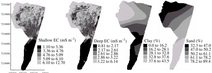
With the semivariograms, surface maps could be generated for each variable using kriging interpola-tion. Figure 1 presents some of these maps, specifically for the shallow (0–0.3 m) and deep EC values (0–0.9 m), and for clay and sand contents. To the observer, the similarity between these maps should be clear. The “softer” appearance of the distribution of soil texture in relation to soil EC is caused by the sample density dif-ference. A visual inspection of these maps indicates a good agreement between both. This relationship between EC and soil texture was previously reported by Williams & Hoey (1987) and, recently, in a field near by this one, by Machado et al. (2006).
The correlation between soil EC for the shal-low and deep readings and soil physicochemical at-tributes was evaluated based on the generated surface maps (Table 3). Regarding the relation between EC in the shallow reading and the soil attributes analyzed in the laboratory, a number of medium and strong cor-relations could be identified between EC and P, OM, pH, K, Ca, Mg, SB, CEC, V%, clay, and sand. Sev-eral medium and high-intensity correlations were also verified between deep-reading EC and the following soil attributes: P, OM, pH, K, Ca, Mg, SB, CEC, V%, clay, and sand. Specifically, the strong relation between EC and soil texture is a promising indication toward its use to define soil management zones in the study area.
From the correlations between soil variables and soil EC at both depths, a number of correlations with intensities from moderate to strong can be iden-tified between them. These interactions are limiting fac-tors for the use of simple correlation analysis in the interpretation of these data. Principal component analy-sis was then used to reduce the number of variables, which are to be used later to generate management zones, without loss of relevant information. Trials were also done to evaluate whether EC, at both depths, could somehow help to define soil management zones (Table 4).
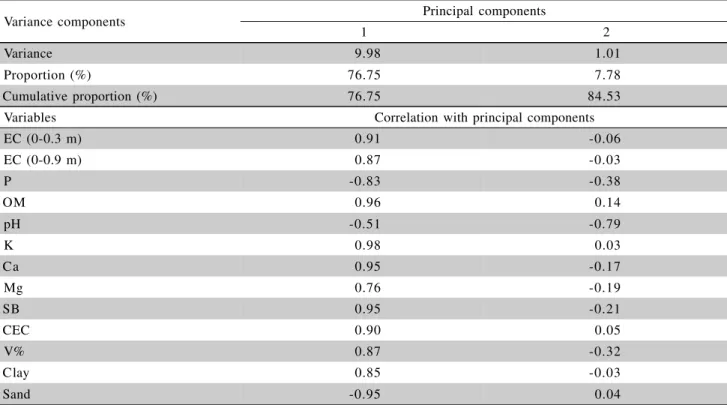
Two PCs were selected among the total set of 13 original variables, which together explained 84.5% of the total variance of those data. The first PC (re-sponsible for 76.7% of variability) is strongly
influ-Table 3 - Coefficients of correlation between shallow (0 - 0.3 m) and deep-reading (0 - 0.9 m) soil EC and other soil physicochemical attributes (OM = organic matter; SB = sum of bases; CEC = cation exchange capacity; V = base saturation).
Variables P OM pH K Ca Mg SB CEC V% Clay Sand
EC (0-0.3 m) -0.68 0.86 -0.41 0.87 0.84 0.63 0.84 0.77 0.76 0.75 -0.86
EC (0-0.9 m) -0.64 0.82 -0.42 0.81 0.81 0.60 0.81 0.74 0.73 0.66 -0.79
Figure 1 - Shallow (0 – 0.3 m) and deep-reading (0 – 0.9 m) soil EC maps, and soil clay and sand content maps.
7219200
7219000
7218800
7218600
7218400
7218200
7218000
579200 579400 579600 57980
Shallow EC (mS m–2) 1.10 to 3.36 3.36 to 4.76 4.76 to 5.09
5.09 to 6.10 6.10 to 12.70
Deep EC (mS m–2 0.81 to 2.17 2.17 to 2.61 2.61 to 2.86 2.86 to 3.22 3.22 to 6.14
) Clay (%) 0.0 to 16.2 16.2 to 28.1 28.1 to 32.8 32.8 to 37.6 37.6 to 43.5
Sand (%) 32.3 to 47.0 47.0 to 50.2 50.2 to 61.1
enced by all original variables, with the exception of pH. This can be viewed as the inherent fertility poten-tial of the soil. Due to the direct relation between the original variables and this PC, regions with higher val-ues for this PC are the most fertile. Furthermore, it is important to highlight the great intensity of the influ-ence of both shallow and deep soil EC readings on this PC (having correlations with the first principal com-ponent equal to 0.91 and 0.87, respectively), indicat-ing the importance of this information in helpindicat-ing to ex-plain the soil general physicochemical spatial variabil-ity of the area. The second PC showed a more intense relation with pH only, approximately the contrary of the first PC, for which the relative influence of pH was low.
In the following step, the fuzzy k-mean con-tinuous classification technique was used to define soil management zones based on the two PCs pre-sented in Table 4. The Euclidean distance criterion and a fuzzy exponent of 1.2 were used. The Fuzzy Performance Index (FPI) and the Modified Partition Entropy (MPE) were used to determine the optimal number of management zones in each area. These two indices are provided by the FuzMe program it-self (Minasny & McBratney, 2000). The optimal num-ber of cluster classes (management zones) is then defined as the number at which these two indices reach their minimum value (Fridgen et al., 2001). FPI and MPE indices reached a minimum value for a
di-vision of the area into three classes (three manage-ment zones), indicating that this is the optimal num-ber of soil management zones based on the sampled variables (Figure 2).
The two previously selected PCs were then submitted to fuzzy classification, where an individual could have total, partial, or null participation in each of the different classes. The maps for the three clus-ters with their respective management zones resulting from this classification are presented in Figure 3.
The final fuzzy classification result provides participation function values for each individual (da-tum) in the original set of data for each of the gener-ated classes. This function may assume values between 0.0 (no possibility of participation in the class) and 1.0 (total participation in the class). In this study, the clus-ter of individuals whose participation function in the
Variance components Principal components
1 2
Variance 9.98 1.01
Proportion (%) 76.75 7.78
Cumulative proportion (%) 76.75 84.53
Variables Correlation with principal components
EC (0-0.3 m) 0.91 -0.06
EC (0-0.9 m) 0.87 -0.03
P -0.83 -0.38
OM 0.96 0.14
pH -0.51 -0.79
K 0.98 0.03
Ca 0.95 -0.17
Mg 0.76 -0.19
SB 0.95 -0.21
CEC 0.90 0.05
V% 0.87 -0.32
Clay 0.85 -0.03
Sand -0.95 0.04
Table 4 - Principal components analysis for the soil physicochemical variables collected (OM = organic matter; SB = sum of bases; CEC = cation exchange capacity; V = base saturation).
Figure 2 - Cluster performance graph as a function of number of classes.
0 0.05 0.1 0.15 0.2
2 3 4 5 6 7 8
Number of classes
Index
Table 5 - Mean soil physicochemical variables per management zone (OM = organic matter; SB = sum of bases; CEC = cation exchange capacity; V = base saturation).
*ECs = shallow-reading electrical conductivity (0 - 0.3 m); ECd = deep-reading electrical conductivity (0 - 0.9 m); Clay = clay content; Sand = Sand content. †Variable means in the same column followed by different letters are different between management zones by Tukey HSD test for unequal samples (P = 0.05).
Zone Variables*†
ECs ECd P OM pH K Ca Mg SB CEC V% Clay Sand
1 5.2b 2.8b 40.2b 40.5a 4.8a 2.0c 2.7b 29.6b 15.0b 47.0b 46.4b 29.7b 57.9b
2 2.4a 1.7a 93.1c 20.1b 5.0c 1.0a 1.3a 19.4a 9.6a 29.5a 41.5a 13.1a 83.9c
3 6.6c 3.4c 38.9a 46.7c 4.9b 1.6b 3.2c 37.0c 20.2c 61.7c 51.7c 37.5c 43.7a
same given class was higher than 0.50 were consid-ered belonging to a distinct management zone, as can be seen in maps from A through C in Figure 3.
The spatial continuity of the management zones presented in Figure 3 is quite large, and may be considered an indication that the classification was suc-cessful, since it will later facilitate management opera-tions in the area. It is interesting to compare the man-agement zone maps for this area against the spatial dis-tribution maps for clay and sand (Figure 1). Based on the comparison between these information layers it becomes easy to notice the influence of soil texture on the soil’s behavior. Due to the relation between EC measurements at both depths with texture (r = 0.75 and 0.66 for the ratios between shallow and deep EC readings with soil clay content, respectively), the le-gitimacy of this information in defining management zones for this area can be observed.
The last step of the study consisted in run-ning an analysis of variance (ANOVA) in order to verify whether there were differences between the EC variables at both depths and soil physico-chemical characteristics among the different
manage-ment zones created by the fuzzy k-means algorithm. The greater the differences the more the validity of the performed division is confirmed; the differ-ences also confirm whether the process of reduction of the number of variables (principal components analysis) was able to suitably express their spatial variability model. The ANOVA results for soil vari-ables among management zones are presented in Table 5.
There is a considerable relation between shal-low and deep soil EC and soil clay content, with the means for these variables among zones arranged in as-cending order. In addition, most soil attributes fol-lowed this tendency, with zone 3 showing the highest soil fertility indices. The differences found between zones for all these variables were significant, demon-strating the viability of the proposed classification, and indicating that a differentiated management is possible between zones for the sampled soil attributes. How-ever, more researches showing the utility of EC with the same objective for other locations with soil char-acteristics diverse from those found in this study are needed.
Figure 3 - Maps showing the spatial distribution of participation function values for each individual in the three classes generated after classification by the fuzzy-k-means algorithm of two principal components selected and corresponding map showing the resulting management zones.
0.25 Class 2 0.00 to 0.25 0.25 to 0.50 0.50 to 1.00
7219200
7219000
7218800
7218600
7218400
7218200
7218000
579200 579400 579600 579800
Class 1 0.00 to 0.25 0.25 to 0.50
0.50 to 1.00
Class 3 0.00 to 0.25 0.25 to 0.50
Received December 11, 2006 Accepted August 29, 2008
CONCLUSIONS
A manner to define differentiated soil manage-ment zones was achieved in this work using EC and other soil properties, in addition to geostatistics, prin-cipal component analysis, and fuzzy logic to handle the data. It was proved to be a viable procedure for the area, allowing the delimitation of homogeneous and dis-tinct regions among them with reference to the soil attributes and the resulting three management zones represent a reasonable number for practical use. The relations between shallow and deep soil EC and clay content indicated the viability of using this informa-tion to delineate soil management zones, since it is the main factor controlling the spatial variability of other soil fertility indicators.
ACKNOWLEDGMENTS
This project was conducted with financial sup-port from FAPESP and CNPq, and with significant par-ticipation of ABC Foundation.
REFERENCES
AFIFI, A.A.; CLARK, V. Computer-aided multivariate
analysis. New York: Chapman & Hall, 1996. 455 p. BURROUGH, P.A.; GAANS, P.F.M. van; HOOTSMANS, R.
Continuous classification in soil survey: spatial correlation, confusion and boundaries. Geoderma, v.77, p.115-135, 1997. FRIDGEN, J.J.; KITCHEN, N.R.; SUDDUTH, K.A. Variability of soil and landscape attributes within sub-field management zones. In: INTERNATIONAL CONFERENCE ON PRECISION AGRICULTURE, 5., Bloomington, 2000. Proceedings. Madison: ASA-CSSA-SSSA, 2001. CD-ROM.
ISAAKS, E.H; SRIVASTAVA, R.M. Applied geostatistics. New York: Oxford University Press, 1989. 561p.
LUCHIARI JR., A.; SHANAHAN, J.; FRANCIS, D.; SCHLEMMER, M.; SCHEPERS, J; LIEBIG, M.; SCHEPERS A.; PAYTON, S. Strategies for establishing management zones for site specific nutrient management. In: INTERNATIONAL CONFERENCE ON PRECISION AGRICULTURE, 5., Bloomington, 2000.
Proceedings., Madison: ASA-CSSA-SSSA, 2001. CD-ROM. MACHADO, P.L.O.A.; BERNARDI, A.C.C.; VALENCIA, L.I.O.;
MOLIN, J.P.; GIMENEZ, L.M.; SILVA, C.A.; ANDRADE, A.G.A.; MADARI, B.E.; MEIRELLES, M.S.P.M. Mapeamento da condutividade elétrica e relação com a argila de Latossolo sob plantio direto. Pesquisa Agropecuária Brasileira, v.41, p.1023-1031, 2006.
McBRIDE, R.A; GORDON, A.M; SHRIVE, S.C. Estimating forest soil quality from terrain measurements of apparent electrical conductivity. Soil Science Society of American Journal, v.54, p.255-260, 1990.
MINASNY, B.; McBRATNEY, A.B. FuzME version 2.1. 2000. Available at: http://www.usyd.edu.au/su/agri/acpa. Accessed 23 Feb. 2002.
NADLER, A; FRENKEL, H. Determination of soil solution electrical conductivity from bulk soil electrical conductivity measurements by the four electrode method. Soil Science Society of
American Journal, v.44, p.1216-1221, 1980.
SHEETS, K.R; HENDRICKX, J.M.H. Noninvasive soil water content measurement using electromagnetic induction. Water Resources Research, v.31, p.2401-2409, 1995.