www.the-cryosphere.net/8/1297/2014/ doi:10.5194/tc-8-1297-2014
© Author(s) 2014. CC Attribution 3.0 License.
Tracing glacier changes since the 1960s on the south slope of
Mt. Everest (central Southern Himalaya) using optical satellite
imagery
S. Thakuri1,3, F. Salerno1,2, C. Smiraglia3, T. Bolch4,5, C. D’Agata3, G. Viviano1, and G. Tartari1
1National Research Council, Water Research Institute (IRSA-CNR), Brugherio, Italy 2Ev-K2-CNR Committee, Via San Bernardino, 145, Bergamo 24126, Italy
3Department of Earth Sciences "Ardito Desio", University of Milan, Milan, Italy 4Department of Geography, University of Zurich, Zurich, Switzerland
5Institute for Cartography, Technische Universität Dresden, Dresden, Germany
Correspondence to:S. Thakuri ([email protected])
Received: 1 September 2013 – Published in The Cryosphere Discuss.: 8 November 2013 Revised: 11 March 2014 – Accepted: 12 June 2014 – Published: 22 July 2014
Abstract. This contribution examines glacier changes on the south side of Mt. Everest from 1962 to 2011 consid-ering five intermediate periods using optical satellite im-agery. The investigated glaciers cover∼400 km2and present
among the largest debris coverage (32 %) and the highest elevations (5720 m) of the world. We found an overall sur-face area loss of 13.0±3.1 % (median 0.42±0.06 % a−1),
an upward shift of 182±22 m (3.7±0.5 m a−1) in
snow-line altitude (SLA), a terminus retreat of 403±9 m (median 6.1±0.2 m a−1), and an increase of 17.6±3.1 % (median
0.20±0.06 % a−1) in debris coverage between 1962 and
2011. The recession process of glaciers has been relentlessly continuous over the past 50 years. Moreover, we observed that (i) glaciers that have increased the debris coverage have experienced a reduced termini retreat (r=0.87,p <0.001). Furthermore, more negative mass balances (i.e., upward shift of SLA) induce increases of debris coverage (r=0.79,
p <0.001); (ii) since early 1990s, we observed a slight but statistically insignificant acceleration of the surface area loss (0.35±0.13 % a−1 in 1962–1992 vs 0.43±0.25 % a−1 in
1992–2011), but an significant upward shift of SLA which increased almost three times (2.2±0.8 m a−1in 1962–1992
vs 6.1±1.4 m a−1in 1992–2011). However, the accelerated
shrinkage in recent decades (both in terms of surface area loss and SLA shift) has only significantly affected glaciers with the largest sizes (>10 km2), presenting accumulation zones at higher elevations (r=0.61, p <0.001) and along
the preferable south–north direction of the monsoons. More-over, the largest glaciers present median upward shifts of the SLA (220 m) that are nearly double than that of the smallest (119 m); this finding leads to a hypothesis that Mt. Everest glaciers are shrinking, not only due to warming temperatures, but also as a result of weakening Asian monsoons registered over the last few decades. We conclude that the shrinkage of the glaciers in south of Mt. Everest is less than that of others in the western and eastern Himalaya and southern and east-ern Tibetan Plateau. Their position in higher elevations have likely reduced the impact of warming on these glaciers, but have not been excluded from a relentlessly continuous and slow recession process over the past 50 years.
1 Introduction
Figure 1. (a)Location of the study area: the Sagarmatha National Park (SNP), where the abbreviations CH, WH, EH, and TP represent the central Himalaya, the western Himalaya, the eastern Himalaya, and the Tibetan Plateau, respectively (suffixes -N and -S indicate the northern and southern slopes).(b)Focused map of the SNP in 2011 showing the distribution of 29 glaciers considered in this study with a surface area
>1 km2.(c)The hypsometric curve of the glaciers in 2011.
(Scherler et al., 2011; Salerno et al., 2012), an effect that has often been neglected in predictions of future water availabil-ity.
Some previous studies have discussed that debris-covered glaciers behave unlike clean glaciers (Nakawo et al., 1999; Benn et al., 2012). Scherler et al. (2011) studied debris-covered glaciers around the Himalayan range for a period of 2000–2008 and showed that heavy debris coverage influ-ences terminus behaviors by stabilizing the terminus posi-tion change. However, Kääb et al. (2012), in a comprehen-sive study on the glacier mass change from 2003–2008 in the Himalaya, suggested that debris-covered ice thins at a rate similar to that of exposed ice. Significant mass loss despite thick debris cover was also reported by Bolch et al. (2011), Nuimura et al. (2012), and Pieczonka et al. (2013). Hence, the relation of length changes to mass balance is even weaker for debris-covered than for debris-free glaciers and there is a need for further assessment of the role of debris mantles.
This contribution examines the glacier changes on the south side of Mt. Everest as part of an effort to better define the glaciers status in the Himalaya. We extend the analysis of Salerno et al. (2008) carried out on the glacier surface area change (1Surf) on two historical maps (the period ranging from the 1950s to 1992). First of all, we cover a longer period (ranging from the 1960s to 2011) increasing furthermore the temporal resolution with six medium-high resolution satellite imagery, with the assistance of all available historical maps. Secondly, we make a complete analysis of terminus position change (1Term), shift of snow-line altitude (1SLA), and changes in debris coverage (1DebrisCov). The results are compared with those obtained in previous studies in this area and along the Himalaya and the Tibetan Plateau range. We
conclude by attempting to link the observed impacts with the climate change drivers.
2 Study area
The current study is focused on the Mt. Everest region, and in particular in the Sagarmatha (Mt. Everest) National Park (SNP) (27.75◦to 28.11◦N; 85.98◦to 86.51◦E) that lies in eastern Nepal in the southern part of the central Himalaya (CH-S) (Fig. 1a). The park area (1148 km2), extending from an elevation of 2845 m at Jorsale to 8848 m a.s.l., covers the upper catchment of the Dudh Koshi river (Manfredi et al., 2010; Amatya et al., 2010). Land cover classification shows that less than 10 % of the park area is forested (Salerno et al., 2010a; Bajracharya et al., 2010). The SNP is the world’s highest protected area with over 30 000 tourists in 2008 (Salerno et al., 2010b, 2013). This region is one of the heav-ily glacierized parts of the Himalaya with almost one-third of the park territory characterized by ice cover. Bajracharya and Mool (2009) indicate that there are 278 glaciers in the Dudh Koshi Basin, with 40 glaciers accounting for most of the glacierized area (70 %) and all of these being valley-type. Most of the large glaciers are debris-covered type, with their ablation zone almost entirely covered by surface debris (Fig. 1b).
park including 17 proglacial lakes, 437 supraglacial lakes, and 170 unconnected lakes. In general, they observed that supraglacial lakes occupy from approximately 0.3 to 2 % of downstream glacier surfaces.
The glacier hypsometric curve plotted, using the glacier outlines of 2011 and the Advanced Spaceborne Thermal Emission and Reflection Radiometer Global Digital Eleva-tion Model (ASTER GDEM, a product of METI and NASA), Version 2 indicates that the glacier surfaces are distributed from around 4300 m to above 8000 m a.s.l. with more than 75 % glacier surfaces lying between 5000 m and 6500 m a.s.l. (Fig. 1c); the area-weighted mean elevation of the glacier is 5720 m a.s.l in 2011. These glaciers are identified as summer-accumulation type fed mainly by summer precipi-tation from the South Asian monsoon system, whereas the winter precipitation caused by mid-latitude westerly wind is minimal (Ageta and Fujita, 1996; Tartari et al., 2002). The prevailing direction of the monsoons is S–N and SW– NE (Rao, 1976; Ichiyanagi et al., 2007). Based on the me-teorological observations at the Pyramid Laboratory Ob-servatory (5050 m a.s.l.), the mean annual air temperature is −2.5±0.5◦C. In summer (June–September), air
tem-perature is typically above 0◦C, the maximum occurs in July, and shows a typical variation associated with cloudi-ness. In contrast, thermal range is very high during win-ter owing to less cloudy conditions. In winwin-ter, the maxi-mum daily temperature is usually below 0◦C, especially in February, the coldest month. Mean total annual precipitation is 516±75 mm a−1, with about 88 % of the annual amount
recorded during the summer months (June–September). The vertical gradients of temperature, precipitation and solar radi-ation has been calculated using meteorological stradi-ations from 90 to 5600 m a.s.l. (data from Nepal Department of Hydrol-ogy and MeteorolHydrol-ogy – DHM – and Ev-K2-CNR Commit-tee). We found a temperature lapse rate of−0.0059◦m−1, a
solar radiation gradient of+0.024 W m−2m−1, valid for the
2800–5000 m a.s.l. elevation range, and for pre- and post-monsoon months, while the post-monsoon period is affected by high cloud cover. The precipitation increases with altitude by+0.067 mm [month] m−1until around 2800 m a.s.l.
after-wards it starts decreasing (−0.017 mm [month] m−1).
3 Data and methods 3.1 Data sources
The analyses of 1Term, 1Surf, 1SLA and 1DebrisCov of Mt. Everest glaciers were performed from 1962 to 2011 using satellite imagery, with the assistance of all available historical maps (Table 1). We analyzed the glacier changes within five periods: 1962–1975, 1975–1992, 1992–2000, 2000–2008, and 2008–2011.
All satellite data were acquired after the monsoon season during the period from October-December. These images are
characterized by low cloud cover and correspond to time just after the end of the snow accumulation and ablation period for that year; this allows for homogeneous comparisons (Paul et al., 2009). These months also coincides with the minimum ablation period on glaciers. The declassified Corona KH-4 (hereafter Corona-62) was used as a main data source for the base year of the analysis (1962). The Khumbu Himal map of late 1950s (Schneider, 1967; Salerno et al., 2008; hereafter KHmap-50s) and the topographic map of the Indian survey of 1963 (hereafter TISmap-63) were used to complement the results achieved using Corona-62 since the Corona-62 had the complex image geometry and absence of satellite camera specification for its rectification. The KHmap-50s has clear glacier boundaries, but the TISmap-63 has less discernible glacier outlines; thus, the first map was used for analysis re-lated to1Surf,1Term, and1SLA, while use of the TISmap-63 was limited to1Term. The Corona KH-4B (Corona-70) image covers only a small portion of the northeast part of the study area. Therefore, the Landsat MultiSpectral Scan-ner (MSS) (1975) (Landsat-75) was used as the main data source, although its pixel resolution is significantly lower. Moreover, we compared the 1992 Landsat Thematic Map-per (TM) scene (Landsat-92) with the official topographic map of Nepal from same year (OTNmap-92). Concerning the more recent years, we used Landsat ETM+scenes from 2000
(Landsat-00), 2011 (Landsat-11), and an ALOS AVNIR-2 scene (ALOS-08).
The ASTER GDEM, vers. 2 tiles for the Mt. Ever-est region were downloaded from http://gdem.ersdac. jspacesystems.or.jp. The vertical and horizontal accuracy of the GDEM are∼20 m and∼30 m, respectively (http://www. jspacesystems.or.jp/ersdac/GDEM/E/4.html). We decided to use the ASTER GDEM instead of the Shuttle Radar Topog-raphy Mission (SRTM) Digital Elevation Model (DEM) con-sidering the higher resolution (30 m and 90 m, respectively) and the large data gaps of the SRTM DEM in this study area (Bolch et al., 2011). Furthermore, the ASTER GDEM shows better performance in mountain terrains (Frey et al., 2012).
3.2 Gap fill and pan-sharpening of Landsat SLC-off data
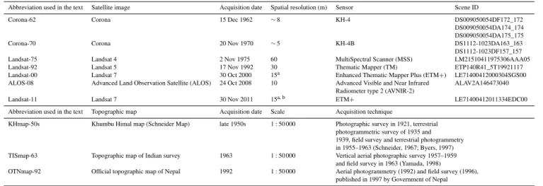
Table 1.Data sources used in this study.
Abbreviation used in the text Satellite image Acquisition date Spatial resolution (m) Sensor Scene ID
Corona-62 Corona 15 Dec 1962 ∼8 KH-4 DS009050054DF172_172
DS009050054DA174_174 DS009050054DA175_175
Corona-70 Corona 20 Nov 1970 ∼5 KH-4B DS1112-1023DA163_163
DS1112-1023DF157_157 Landsat-75 Landsat 4 2 Nov 1975 60 MultiSpectral Scanner (MSS) LM21510411975306AAA05 Landsat-92 Landsat 5 17 Nov 1992 30 Thematic Mapper (TM) ETP140R41_5T19921117 Landsat-00 Landsat 7 30 Oct 2000 15a Enhanced Thematic Mapper Plus (ETM+) LE71400412000304SGS00 ALOS-08 Advanced Land Observation Satellite (ALOS) 24 Oct 2008 10 Advanced Visible and Near Infrared ALAV2A146473040
Radiometer type 2 (AVNIR-2)
Landsat-11 Landsat 7 30 Nov 2011 15a, b ETM+ LE71400412011334EDC00 Abbreviation used in the text Topographic map Acquisition date Scale Acquisition technique
KHmap-50s Khumbu Himal map (Schneider Map) late 1950s 1:50 000 Photographic survey in 1921, terrestrial photogrammetric survey of 1935 and 1939, field survey and terrestrial photogrammetry in 1955–1963 (Schneider, 1967; Byers, 1997) TISmap-63 Topographic map of Indian survey 1963 1:50 000 Vertical aerial photographic survey 1957–1959
and field survey in 1963 (Yamada, 1998)
OTNmap-92 Official topographic map of Nepal 1992 1:50 000 Aerial photogrammetry (1992) and field survey (1996), published in 1997 by Government of Nepal aPan-sharpened images;
bSLC-off image.
Figure 2.Glacier delineation in(a)panchromatic Corona-62;(b)SLC-off gap filled Landsat-11. The stripes in the images are meant for mean length change calculation.
panchromatic band (15 m) acquired by same satellite and on the same date.
3.3 Data registration
All of the imagery and maps were co-registered in the same coordinate system of WGS 1984 UTM Zone 45. The Land-sat scenes were provided in standard terrain-corrected level (Level 1T) with the use of ground control points (GCPs) and necessary elevation data (https://earthexplorer.usgs.gov). The ALOS-08 image used here was orthorectified and cor-rected for atmospheric effects in Salerno et al. (2012). The Corona images were co-registered and rectified through the polynomial transformation and spline adjustment using more than 120 known GCPs obtained from the reference ALOS-08 image, including mountain peaks, river crossings, and identi-fiable rocks (Grosse et al., 2005; Lorenz, 2004). The polyno-mial transformation uses a least squares fitting algorithm and
ensures the global accuracy of images (Rosenholm and Ak-erman, 1998), but does not guarantee local accuracy, whereas the spline adjustment improves for local accuracy, which is based on a piecewise polynomial that maintains continuity and smoothness between adjacent polynomials (Kresse and Danko, 2011). The overall root mean square error (RMSE) of GCPs in Corona registration was around 8 m. The ERDAS IMAGINE® software was used for processing the Corona image. The images were resampled to new pixel size (8 m) using the nearest neighbor method, most commonly applied resampling technique (Thompson et al., 2011; Brahmbhatt et al., 2012).
3.4 Interpretation and mapping of glacier features
Paul et al., 2013). Though few automated approaches to map the debris-covered parts exist, the results are less accurate and need intensive manual post-correction (Paul et al., 2004; Bhambri et al., 2011; Rastner et al., 2013). In this study, the glacier outlines were manually delineated using an on-screen digitizing method based on visual interpretation and false-color composite (FCC) developed from multispectral bands and assisted by the GDEM (Fig. 2a and b). The well es-tablished the band ratio (TM4/TM5) technique (Paul et al., 2004) was used to obtain a clear vision of snow and ice por-tion that assisted in the manual digitizapor-tion. In the ablapor-tion part of the glacier where debris mantles are present, the delin-eation of the outline was performed by identifying lateral and frontal moraine and using the thermal band for the Landsat TM and ETM images. Streams issuing from beneath glacier were used as additional indication of its boundary.
For the 1Term calculation, a band of stripes with a dis-tance of 50 m between each stripe in the band was drawn parallel to the main flow direction of the glacier (Fig. 2), and the1Term was calculated as the average length of the inter-section of the stripes with the glacier outlines (cf. Koblet et al., 2010; Bhambri et al., 2012).
The snow lines were retrieved manually from each satel-lite image and map. The snow lines on glaciers were dis-tinguished from the images as the boundary between the bright white snow and the darker ice by visual interpreta-tion and using FCC (Karpilo, 2009). The kinematic “Hess method” (Hess, 1904) was used to identify the snow line in the KHmap-50s, which involves the delineation of the boundary between the accumulation and ablation zone in a glacier using the inflection of elevation contour lines on the topographic map (Leonard and Fountain, 2003). Then, the SLA, as a measure of equilibrium-line altitude (ELA; Mc-Fadden et al., 2011; Rabatel et al., 2012), was calculated as the average altitude of the identified snow line using the ASTER GDEM. The SLA derived from the “Hess method” for the map represents the long-term ELA and, thus, does not indicate the position of the snow line in a particular year. However, the snow line position obtained from satellite im-agery represents the transient snow line of the year that varies along the year, but remains stable after the end of summer, corresponding to the end of the ablation season (Rabatel et al., 2005; Pelto, 2011). The map-based SLA was useful for understanding the representativeness of the snow line posi-tion derived from the Corona image, which has some limita-tions for accurately identifying the snow line because of its panchromatic nature.
The ASTER GDEM along with glacier outlines were used to derive morphological features (slope, aspect, elevation). The mean elevation, aspect, and slope of each glacier were computed as arithmetic mean of each pixel of the GDEM in-tersected by the glacier outline. Concerning the glacier iden-tification and cataloging, we followed the classification of Salerno et al. (2008), which in turn is based on the inventory of the International Centre for Integrated Mountain
Develop-ment (ICIMOD) (Mool et al., 2001). In agreeDevelop-ment with this study, we named only those glaciers whose area exceeded a threshold of 1 km2. In this way, we identified 29 glaciers, while the smaller glaciers (<1 km2) were categorized into “other glaciers” group.
3.5 Uncertainty of measurement
The measurement accuracy of the position of a single point in the space using GIS (geographical information system) is limited by resolution of source data used (i.e., the scale factor for cartography and the pixel resolution for satellite image), defined as LRE (linear resolution error), and by the error of referencing (RE, registration error). This approach is usually adopted in studies of glacial front (1Term) (Hall et al., 2003; Ye et al., 2006). Concerning the glacier surface and debris coverage, the uncertainty of measurement was calculated as a product of the LRE and the perimeter (l) (Salerno et al., 2012). Then, the uncertainty with 1Surf and 1DebrisCov was derived according to standard error propagation rule, root of sum of squares (RSS) of the mapping error for the single scene. The co-registration errors were approximated and adjusted during the measurement. For further details on methodology adopted here for uncertainty analysis, we refer to Tartari et al. (2008) and Salerno et al. (2012). The eleva-tion error associated with1SLA was estimated as the RSS between of the pixel resolution combined with the mean sur-face slope (Pelto, 2011) and the vertical error associated to the GDEM (20 m). Concerning the uncertainty in the SLA estimation due to temporal variation of surface elevation, we consider them negligible as there was no significant eleva-tion change around SLA (Bolch et al., 2011) compared to the GDEM vertical accuracy, and thus have no impact on the results (Rabatel et al., 2013).
In this study, the uncertainty of measurement ranges from 6 to 30 m for1Term and from 21 to 35 m for1SLA. In both cases, as discussed below and shown in Fig. 3 and Table 2, the magnitude of the uncertainty is relatively low if com-pared with the observed changes, indicating good accuracy of the results. However, the errors associated with1Surf and
1DebrisCov range from approximately 2 to 10 % for both of variables. In particular, Fig. 3 and Table 2 indicate that until early 1990s, this uncertainty, due to low sensor resolution, is high and needs to be carefully considered in the change evaluations.
3.6 The ELA-climate model
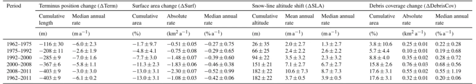
Table 2.Glacier changes from 1962 to 2011 in the Mt. Everest region.
Period Terminus position change (1Term) Surface area change (1Surf) Snow-line altitude shift (1SLA) Debris coverage change (1DebrisCov) Cumulative Median annual Cumulative Absolute Median annual Cumulative Mean annual Median annual Cumulative Absolute Median annual length rate area rate rate altitude rate rate area rate rate (m) (m a−1) (%) (km2a−1) (% a−1) (m) (m a−1) (m a−1) (%) (km2a−1) (% a−1) 1962–1975 −116±30 −6.0±2.3 −1.7±9.7 −0.51±0.05 −0.27±0.75 26±35 2.0±2.7 1.3±2.7 3.8±10.6 0.25±0.01 0.22±0.28 1975–1992 −208±11 −2.6±1.9 −4.8±4.1 −0.75±0.08 −0.29±0.65 66±25 2.4±2.2 2.6±2.2 5.7±4.4 0.10±0.01 0.19±0.68 1992–2000 −285±9 −7.0±1.6 −7.7±3.0 −1.48±0.07 −0.39±0.60 94±22 3.5±3.2 2.3±3.2 8.8±4.0 0.35±0.02 0.28±0.72 2000–2008 −367±6 −5.8±1.1 −11.3±2.3 −1.83±0.06 −0.46±0.38 151±21 7.1±2.7 6.7±2.7 15.8±2.6 0.76±0.03 0.68±0.56 2008–2011 −403±9 −3.0±3.0 −13.0±3.1 −2.30±0.07 −0.52±0.99 182±22 10.6±7.3 8.7±7.3 17.6±3.1 0.55±0.02 0.55±1.19 1962–2011 −403±9 −6.1±0.2 −13.0±3.1 −1.08±0.03 −0.42±0.06 182±22 3.7±0.5 3.9±0.5 17.6±3.1 0.32±0.01 0.20±0.06
rate, mass balance and radiation gradients, latent heat of fu-sion and length of melting season.
The model is expressed as,
∂bw
∂z 1h+δbw= T L
∂R
∂z1h+δR+γ
∂Ta
∂z 1h+δTa
, (1)
where 1h= an observed change in ELA (m), T = length of melting season (d), L= latent heat of fusion (kJ kg−1),
γ= constant (MJ m−2d−1K−1), ∂bw∂z= mass balance
gradient (kg m−2 m−1), ∂Ta∂z= temperature lapse rate
(K m−1),∂R/∂z= net radiation gradient (MJ m−2m−1d−1),
δTa= bias in air temperature (K),δbw= bias in mass balance
(kg m−2), andδR= bias in net radiation (MJ m−2d−1). We
applied the model using the temperature lapse rate and the net radiation gradient calculated for this case study as described above, the mass balance gradient of 5±1 mm w.e. a−1m−1
provided by Fujita et al. (2006),T= 100 d;L= 334 kJ kg−1,
γ= 1.7 MJ m−2d−1K−1as described in Kuhn (1981). Concerning the limitations of this model, we need first of all to consider that the SLA as a proxy to ELA; we as-sume that there is little, or no ablation during winter sea-son. Furthermore, this model just considers a single mass balance gradient value, while some authors, e.g., Wagnon et al. (2013) recently found an average mass balance gradi-ent of 4.5 mm w.e. a−1m−1for Mera Glacier (in the Dudh Koshi Basin), similar to the gradient provided by Fujita et al. (2006), but point out its variability in relation to local to-pographic conditions.
3.7 Statistical analysis
The normality of the data is tested using the Shapiro–Wilk test. The null hypothesis for the Shapiro–Wilk test is that samples x1, x2. . . .xn belong to a normally distributed pop-ulation. If thep value (p)>0.05, we consider the series to be normally distributed; otherwise, it is not normal (Shapiro and Wilk, 1965). We used the paired t test for comparing the means of two series. The null hypothesis is that the differ-ence between paired observations is zero (p <0.05) (Wal-ford, 2011). If the series were not normal, we first used a log transformation to apply the paired t test for a normally distributed series. The parallelism between the regressions of SLAs time series is tested by the analysis of covariance
(ANCOVA) (Dette and Neumeyer, 2001). All tests are im-plemented in the R software environment.
4 Results
Table 2 provides a general summary of the changes that oc-curred from 1962 to 2011. Our main findings, however, are visualized in Fig. 3, which has been subdivided into four sections (a–d), corresponding to four selected indicators of change (terminus, surface area, SLA, and debris coverage). The spatial differences are presented on the right side of each section, and the temporal changes are shown on the left side. On the left side, in the upper panel of each section, the box plots show the annual rates of change for the analyzed period, while the cumulative changes and their associated uncertain-ties are presented in the lower panels. All data presented and discussed in this paper are reported in Tables S1 and S2 of the Supplement.
4.1 Glacier terminus position change
Overall, the Mt. Everest glaciers experienced a1Term of
−403±9 m (σ=533 m) (Fig. 3a2 and Table 2) as the mean
(−301±9 m as median), corresponding to an annual mean
rate of −8.2±0.2 m a−1 (σ=10.8 m a−1) and a median value equal to−6.1±0.2 m a−1from 1962 to 2011 (Fig. 3a1
and Table 2). We found that the distribution of the annual retreat rates in all observed periods (Shapiro–Wilk test) was always far from normal because a few glaciers experienced a retreat that was much higher than the retreat of others (see box plots in Fig. 3a1). Therefore, we consider the median values of1Term to be more representative of the change.
(the weakest significance was found in the 1962–1975 pe-riod). However, when evaluating the possible acceleration, we found no significant differences among the annual rates of change (p >0.1). The result of this test can be further ob-served in Fig. 3a1, considering the distribution of the median annual rates. In fact, the retreat rate has decreased since 1992, although not significantly.
In Fig. 3a3, we can observe the spatial distribution for the overall period of analysis of 1962–2011. We observed that two glaciers (Duwo and Cholo) experienced an over-all advance. These glaciers advanced until 1992, and then they began retreating, similarly to the other glaciers. Fur-thermore, we can observe that most of the western glaciers have retreated more than the eastern ones, except for the Imja Glacier.
As mentioned above, for the first years of the analy-sis, we used the Corona-62 with two topographic maps (KHmap-50s and TISmap-63). Comparing these data sources with the Landsat-75, we observed that the KHmap-50s (6.1±1.9 m a−1) shows a closer mean retreat to
the Corona-62 (8.2±0.2 m a−1) than to the TISmap-63
(13.3±2.6 m a−1), which seems to overestimate the1Term, probably due to inaccurate representation of the glacier boundary in TISmap-63 as found for other topographic maps in the Himalaya (Bhambri and Bolch, 2009).
4.2 Glacier surface area change
The Mt. Everest glaciers experienced a 1Surf of
−52.8±11.0 km2(from 404.6 to 351.8 km2), corresponding
to an overall change of−13.0±3.1 % (−0.27±0.06 % a−1),
from 1962 to 2011 (Fig. 3b2 and Table 2). The mean annual shrinkage rate calculated for each glacier in the period from 1962–2011 was 0.51±0.06 % a−1 (σ= 0.38), and the median rate was 0.42±0.06 % a−1(Fig. 3b1). By testing the
annual loss rate (Shapiro–Wilk test) of each glacier in each observed period, we observed (similarly to the terminus retreat) that it was never normally distributed (see box plots in Fig. 3b1). Therefore, in this case as well, we consider it to be more representative of change in the median values.
We can observe a continuous surface area loss since the 1960s that appears to have accelerated in recent years (Fig. 3b2). In fact, the rate of median annual area loss was 0.27±0.75 % a−1in 1962–1975 and has increased to the rate
of loss of 0.48±0.55 % a−1, in 2000–2011 period (Fig. 3b1).
We thus tested these trend properties using same procedure that we had adopted for evaluating the1Term. In this case, we again first provided a log transformation of the series. We observed that the surface area loss of each period was always significantly different from zero. The weakest signif-icance was found in the 1962–1975 period. In fact, Fig. 3b2 and Table 2 show lower observed surface change (1.7 %) for this period, which, although significant, is associated with the highest uncertainty (9.7 %). However, in evaluating the pos-sible acceleration of the surface area losses, we found slight
but statistically insignificant acceleration of the surface area between the rates of area loss in the 1962–1992 period (me-dian 0.35±0.13 % a−1, 0.015 km2a−1) and the 1992–2011
period (median 0.43±0.25 % a−1, 0.039 km2a−1) indicating that for the 1992–2011 period, each glacier is retreating on average at nearly the double rate than the previous period.
The area loss observed in the first period (1962–1975) us-ing Corona-62 and Landsat-75 was robust usus-ing different data sources, as described in the methods section and shown in Table 1. Comparing the KHmap-50s with the Landsat-75, we obtain a glacier area loss of 0.22±0.64 % a−1,
which is very close to the value obtained using Corona-62 (0.27 % a−1). Moreover, for some glaciers, we were able to substitute high resolution Corona-70 with Landsat-75 to pro-vide information about the accuracy of the Landsat data. The comparison of Corona-62 and Corona-70 provided a mean rate of 0.26 % a−1, confirming that between late 1950s and
early 1970s, the glacier surface losses were very small. Figure 3b3 represents a distinct spatial pattern of glacier
1Surf. All of the glaciers experienced surface area losses between 1962 and 2011. However, the southern glaciers lost higher surface area than the northern glaciers.
4.3 Snow Line Altitude change
Overall, from 1962 to 2011, the SLA of Mt. Everest glaciers shifted upward by 182±22 m (σ= 114) from 5289 m to 5471 m a.s.l.; this increase corresponds to a mean annual rate of 3.7±0.5 m a−1(σ= 2.3) (Fig. 3c1, 3c2, and Table 2). The distribution of the annual rate of the SLA shift in all of the observed periods is in this case normal (Shapiro–Wilk test; see box plots in Fig. 3c1). Therefore, the mean values are suitable for describing the1SLA.
In Fig. 3c2, the overall trend in 1SLA shows a contin-uous upward shift in the last 50 years. In fact, in Fig. 3c1, we can observe that the mean annual upward rate of the SLA was 2.0±2.7 m a−1 in 1962–1975 and achieved the
highest shift rate of 10.6±7.3 m a−1 in the 2008–2011
pe-riod. In this case, we tested the possible continuity and acceleration of trend following the same procedure ap-plied above. We observed a statistically significant upward shift of the SLA (p= 0.02), except during the first period of 1962–1975. Moreover, we found significant differences (p <0.001) in the annual upward shift of the SLA between periods 1962–1992 (mean = 2.2±0.8 m a−1) and 1992–2011
(mean = 6.1±1.4 m a−1).
Figure 3c3 represents the spatial distribution of the SLA for the overall 1962–2011 period. In this case, the spatial pattern is not distinct. The glaciers with the minimum and maximum SLA in 2011 are Cholo (5152 m) and Imja (5742 m), respectively.
very different from the SLA at 5289 m a.s.l., as derived from Corona-62.
4.4 Glacier debris-covered area change
Overall, the debris-covered area has increased by 17.6±3.1 % (0.36±0.06 % a−1) (Fig. 3d2 and
Ta-ble 2) from 1962 to 2011. The mean annual increase rate calculated for each glacier in the 1962–2011 period is 0.28±0.06 % a−1(σ= 0.34), and the median rate is 0.20±0.06 % a−1 (Fig. 3d1). The debris-covered area was
approximately 24.5 % of the total glacier area in 1962 and 32.0 % in 2011. In the same area, Nuimura et al (2012) reported 34.8 % of debris-covered area in 2003–2004. In correspondence of the increase of debris coverage we ob-served the consequent decreasing of debris free area (Fig. S2 in the Supplement). Testing the annual rate of1DebrisCov with the Shapiro–Wilk test, we observed that the increase of the debris-covered area is not normally distributed among all glaciers (Fig. 3d1). Therefore, we also consider the median values to be more representative of change in the case of
1DebrisCov.
In Fig. 3d2, we present the overall 1DebrisCov trend, which indicates a general continuous increase of debris cover area over the last 50 years. The debris cover increase be-gan to be statistically significant for each glacier only af-ter 2000 (p <0.01) years. Evaluating the possible acceler-ation, we found no significant differences among the annual rates of changes (p >0.1). The result of this test can be ob-served in Fig. 3d1, which considers the distribution of me-dian annual rates. Since 2000, the rates of debris-covered area change appear to be decreasing, although not signifi-cantly. Furthermore, we observed a significant relationship between1DebrisCov and1SLA during the 1962–2011 pe-riod (r= 0.79,p <0.01). In this regards, Bolch et al. (2008) observed that debris cover increases during periods of high ablation as more englacially stored debris is exposed. In Fig. 3d3, we can observe the spatial distribution of the debris-covered area (%) in the overall period of analysis of 1962– 2011. We observe that the glaciers experienced an overall in-crease in the debris-covered area, except the glaciers Imja, Kdu_gr125, Langdak, and Langmuche for which local ef-fects could have played important role.
5 Discussion
5.1 Comparison among terminus position change, surface area loss and the relevant mass budget observations
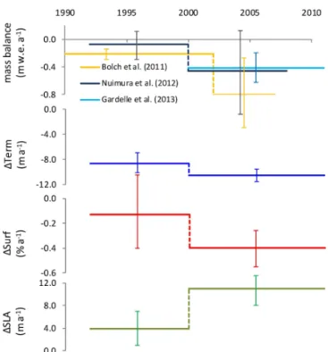
Mass budget measurements are the main index used for climate change impact studies on glaciers, as by Fujita et al. (2006), Bolch et al. (2011), Nuimura et al. (2012), and Gardelle et al. (2013) as this index can be directly linked to climate while length and area change show a delayed signal
Figure 4.Comparison for 10 selected glaciers using the terminus position change (1Term), glacier surface area loss (1Surf), and shift of snow-line altitude (1SLA) calculated in this study and relevant mass downwasting observations of Bolch et al. (2011), Nuimura et al. (2012). Furthermore, the mass balance data of Gardelle et al. (2013) are reported.
(Oerlemans, 2001). However, conducting mass-balance mea-surements is not a trivial task, due to the technical require-ments and practical constraints (Bolch et al., 2012); these measurements are thus not often used in extensive studies. Most of the authors, in fact, analyze glacier terminus position and surface (Bolch et al., 2012; Yao et al., 2012; Kulkarni et al., 2011; Scherler et al., 2011). However, we need to con-sider the limitations of these variables especially for debris-covered glaciers, which experience more downwasting than area loss (Bolch et al., 2008; Tennant et al., 2012). In this re-gard, we decided to compare our findings in terms of1Term,
1Surf, and1SLA with the corresponding mass budget infor-mation provided by other authors to evaluate whether these factors are suitable indices in this context. We present here in Table 3 and Fig. 4 the mass balance data derived from geodetic methods for 10 glaciers located in our study area according to Bolch et al. (2011), Nuimura et al. (2012), and Gardelle et al. (2013). Bolch et al. (2011) and Nuimura et al. (2012) find a higher mass loss rate during the last decade. Furthermore, these estimations are reinforced by the rate pro-vided in Gardelle et al. (2013) for the period (2000-2011).
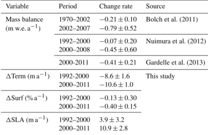
Table 3.Rates of mass balance,1Term,1Surf, and1SLA for 10 common glaciers.
Variable Period Change rate Source
Mass balance 1970–2002 −0.21±0.10 Bolch et al. (2011) (m w.e. a−1) 2002–2007 −0.79±0.52
1992–2000 −0.07±0.20 Nuimura et al. (2012) 2000–2008 −0.45±0.60
2000-2011 −0.41±0.21 Gardelle et al. (2013)
1Term (m a−1) 1992-2000 −8.6±1.6 This study 2000–2011 −10.6±1.0
1Surf (% a−1) 1992–2000 −0.13±0.30 2000–2011 −0.40±0.15
1SLA (m a−1) 1992–2000 3.9±3.2 2000–2011 10.9±2.8
higher in the last decade, as observed using mass budget data. Such behavior is expected given the lag in response time be-cause downwasting leads to more volume loss then retreat (Oerlemans, 2001; Hambrey and Alean, 2004). This com-parison shows that, for this region, the glacier surface area loss and the shift of snow-line altitude (i.e., the shift of late summer snow line) can be considered suitable indicators for a broad description of glacial response to the recent climate change.
5.2 Comparison with other parts of the Himalaya and high-mountain Asia
Bolch et al. (2012) recently noted that length and surface area changes suggest that most Himalayan glaciers have been re-treating since the mid-19th century. Yao et al. (2012) reported the glacier status over the past 30 years in the Himalaya and the Tibetan Plateau. They observed that the shrinkage gener-ally decreases from the Himalaya to the continental interior, and it is most pronounced in the southeastern Himalayan re-gion.
In Nepal, Yao et al. (2012) considered only three bench-mark glaciers for evaluating the Term retreat during the 1974–1999 period and the same set of glaciers analyzed here (Koshi Basin) for evaluating the surface area loss, but for a shorter period (1976–2000) than in the present study. They reported a1Term of 6.9 m a−1based on the three glaciers
lo-cated outside our study area. During a similar period (1975– 2000), we calculated a median retreat of 4.4±0.8 m a−1for
all 29 glaciers and a median retreat of 6.1±0.2 m a−1 for
the 1962–2011 period. Further, in comparing the same set of glaciers and during the same period we found a termini re-treat rate (9 m a−1) lower than the rate (19 m a−1) provided by Bajracharya and Mool (2009), probably due to the higher resolution of data source used in this study (furthermore in Fig. S1 of the Supplement). Concerning the Surf area loss,
Yao et al. (2012) reported a decrease of 0.15 % a−1, while during a similar period (1975–2000), we calculate an area loss of 0.25±0.40 % a−1. We can observe that although the
retreat rates are comparable between the studies, with re-gards to1Surf, we observed a greater area loss; this differ-ence could be because both satellites used in 1975 and 1976 (Landsat MSS) had a broad resolution (60 m) leading to a large uncertainty in the estimates and, hence the studies take the uncertainty into account. Moreover, we sustain that the recent area loss estimation (0.63 % a−1) provided by
Shang-guan et al. (2014) for the same set of glaciers analyzed here during the 1976–2009 period is overestimated probably for the misleading glacier boundary interpretation especially in the upper glacier area in 1976 due to the low resolution Land-sat MSS image and adverse snow conditions, while our inter-pretation is reinforced by the higher resolution of Corona-70 image. Moreover, we point out that the present study cor-responds to zone III of the analysis in Yao et al. (2012), defined by the authors as the central Himalaya and includ-ing both the north (Tibet) and south (Nepal) slopes of the Himalayan range, represented by the Mt. Qomolangma Na-tional Nature Preserve and the Koshi Basin, respectively. The average termini retreat and area loss rates for zone III have been established by the authors at 6.3 m a−1and 0.41 % a−1,
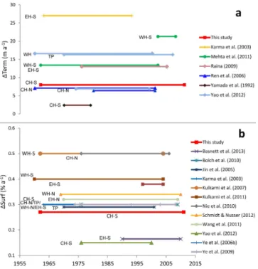
Figure 5.Recent studies on the variations of Himalayan glaciers concerning both the terminus retreat(a)and the surface area loss
(b). Data and references of this figure are presented Table S4 of the Supplement.
during 1962–1992) (Salerno et al., 2008) and 0.12 % a−1 for selected glaciers for the 1962–2005 period (Bolch et al., 2008a), both located in the southern side. Therefore, to ex-plore possible differences in the surroundings of the south slopes of Mt. Everest, we decided to separately consider the northern and southern parts of the central, western and east-ern Himalaya (CH, WH, and EH, respectively, with the suf-fixes -N and -S). Following this scheme, the present case study and all of Nepal are located in CH-S. Evidence from the Tibetan Plateau (TP) is presented separately (Fig. 1a).
Figure 5 reports the most recent studies on the changes of Himalayan glaciers concerning both the terminus re-treat (Fig. 5a) and the area loss (Fig. 5b). In general, we can observe that the CH-S, in terms of both 1Term and
1Surf,registered among the lowest changes of the entire Hi-malaya and the TP. The northern and the southern central Himalaya (CH-N and CH-S) share the lower termini retreat, while the record is held by the CH-S glaciers regarding the lowest area loss, if we consider that the recent study of Bas-nett et al. (2013) on Sikkim Himalaya, although this area is geographically part of EH-S, is adjacent to the eastern CH-S border. The lower 1Term and1Surf observed in CH-S region, compared with the other parts of the Himalaya and the TP, can be ascribed both to the abundance of debris cover (Scherler et al., 2011; Bolch et al., 2012) and to the altitude of these glaciers. Scherler et al. (2011) defined the southern cen-tral Himalaya as the region with the glaciers that contain the highest debris coverage (∼36 %) and considered the
abun-Figure 6.Validation of the SLA trend of 1962-2011 period (green line) for three selected glaciers (Lobuje, Khangri, and Imja) using the satellite imagery reported in Table 1 with additional 20 Landsat ETM+imagery (red points) of 2000–2011 period (shaded region).
dance of debris coverage to be a significant factor in reducing the melt rate of these glaciers, preserving their surfaces from further recession. In this regards, we observed a strong di-rect relationship between1DebrisCov and1Term (divided by the length of the ablation area) (r= 0.87, p <0.01 for 1962–2011 period) which means that the glaciers who have increased the debris coverage have experienced a reduced termini retreat. We remember here that, Bolch et al. (2008a, 2011) noted the highest rate of mass downwasting is located in the transition zone between the active and the stagnant glacier parts of the debris covered glaciers.
However, of no less importance is the altitude of these glaciers. In fact, as reported by Bolch et al. (2012), with a mean elevation of 5600 m a.s.l., the highest glaciers of the Himalayan range are located in CH. In this regards, Wagnon et al. (2013), in the same zone analyzed here (Dudh Koshi Basin) show that a low elevation glacier (Phokalde, 5430 to 5690 m a.s.l.) presents a more negative mass balance (0.72±0.28 m w.e. a−1) than a higher elevation one (Mera,
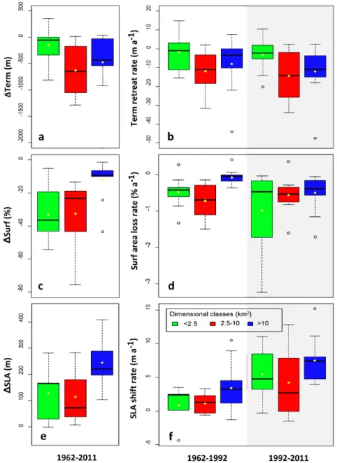
Figure 7.Differences among three-dimensional classes of glaciers (<2.5 km2; 2.5–10 km2;>10 km2) in terms of cumulative changes in the overall 1962–2011 period:(a)terminus retreat (m);(c)surface area loss (%);(e)shift of SLA (m). Differences in terms of annual rate of change between 1962–1992 and 1992–2011 periods;(b)annual terminus retreat rate (m a−1);(d)annual surface area loss rate (% a−1);(f)
shift rate of SLA (m a−1). All percentages refer to the initial year of the analysis (1962).
south slope of Mt. Everest, the area-weighted mean eleva-tion of the glaciers is 5720 m a.s.l in 2011. Therefore, it is highly likely that the summit of the world has preserved these glaciers from excessive melting better than in the other parts of the Himalaya and the TP.
5.3 Snow-line altitude change and climate relation
The snow-line is characterized by seasonal fluctuations (Mernild et al., 2013; Pelto et al., 2013). To avoid the possible risk of introducing this variability into the inter-annual anal-ysis, we enforced our 1962–2011 trend exploiting the
avail-ability of 20 Landsat ETM+imagery for 2000–2011 period.
Bolch et al. (2012), considering the mean elevation as a rough proxy for the ELA, reported an ELA of about 5600 m a.s.l. in CH. For the south slope of the Mt. Ever-est region, Owen and Benn (2005) indicated an elevation of 5200 m a.s.l. for the 1980s, while Asahi (2010) noted an altitude of 5400 m a.s.l. in the early 1990s. In this study, comparing the same years, we observed a SLA position of 5315 m a.s.l. in 1975 and 5355 m a.s.l. in 1992, correspond-ing to a lower shift. Kayastha and Harrison (2008) observed an upward of ELA by 0.9±1.1 m a−1 (29±35 m) during
the 1959–1992 period using the toe-to-headwall altitude ra-tio (THAR) method with TISmap-63 and the aerial photos of 1992, from which the OTNmap-92 was delineated. In a comparable period (1962–1992), we calculated an upward shift of SLA by 2.2±0.8 m a−1(66±24 m) based on
satel-lite data. The difference between the calculation of Kayastha and Harisson (2008) and our calculation is mainly due to dif-ferent methodologies applied and the data set used. Surely, if a suitable scene is available, the SLA derived directly from the satellite imagery is more representative of a specific year than the map-based estimation.
The SLA trend qualitatively indicates the mass-balance variation of glaciers (Chinn et al., 2005). Variations in SLA derived from satellite imagery can be used as a proxy for providing indications of local climate variability (Fujita and Nuimura, 2011; McFadden et al., 2011, Rabatel et al., 2012). In this case study, the SLA is significantly moving up-wards, with an accelerated rate after 1992, indicating that the glaciers in this region are experiencing an increasingly neg-ative mass balance as it is suggested with the mass down-wasting observations of Bolch et al. (2011) and Nuimura et al. (2012) (Fig. 4). The observed upward shift of the snow line could be interpreted as a direct response to high-temperature events, reduced precipitation, or increased so-lar radiation (Hooke, 2005). To evaluate the role of cli-matic drivers in the1SLA,we used the simple ELA-climate model by Kuhn (1981). Using this model, we estimated that for the observed 182 m upward shift of SLA in the 1962– 2011 period, a temperature increase of 1.1◦C, or a precipi-tation decrease of 543 mm, or a solar imbalance increase of 1.8 MJ m−2d−1is required. By reacting to this climate per-turbation, the SLA shifted by 182 m upward.
Concerning the temperatures, on the south slope of Mt. Everest, Diodato et al. (2012) established the longest tem-perature series (1901–2009) for this high elevation area, tak-ing advantage of both land data obtained from the “Pyramid” meteorological observatory (5050 m) for the 1994–2005 pe-riod and gridded temperature data for extending the time se-ries. They observed an increasing trend of 0.01◦C a−1in the last century (+0.9◦C), which can be attributed mainly to the
1980–2008 period (0.03◦C a−1, +0.8◦C). Likewise, Lami
et al. (2010), using only the land data from the “Pyramid” stations (5050 m) for the 1992–2008 period, reported an in-creasing trend of 0.04◦C a−1(+0.7◦C). However, we need
to consider that the recent global warming trend is more
dom-inant in the winter season (Jones and Moberg, 2003). Cook et al. (2003) re-examined a longer Kathmandu mean temper-ature record and compared it with a gridded data set based on records from neighboring northern India; both showed a cooling trend in the monsoon season (June to September) for the 1901–1995 period. Summer cooling trends during the last few decades of the twentieth century have also been docu-mented for the Tibetan Plateau (Liu and Chen, 2000). Ac-cording to Diodato et al. (2012), the temperature in this zone increased by more than+0.8/+0.9◦C during our study
pe-riod (1962–2011), corresponding to 70–80 % of the temper-ature increase required to justify the upward shift of SLA (+1.1◦C), even if, this rise has probably not occurred in the
summer period when the ablation process is concentrated and thus, less impacting on glaciers shrinkage.
For the precipitation, Sharma et al. (2000) showed an in-creased tendency from 1948–1993 in the Dudh Koshi Basin. Additionally, Salerno et al. (2008) noted an increasing trend for higher elevations until the early 1990s. From these years of analysis, many researchers have highlighted a mainly de-creasing trend in the Himalayan range (Wu, 2005; Thomp-son et al., 2006; Naidu et al., 2009). According to Yao et al. (2012), using the Global Precipitation Climatology Project (GPCP) data, the Asian monsoon lost 173 mm in this region for the 1979–2010 period, with a real decreasing trend starting from the early 1990s (mean value between grid 9 and 11 in Fig. S18 of their paper). We have already noted that we would have recorded a decrease of 543 mm if the only factor responsible for the higher SLA were the precipitation. Current knowledge shows that precipitation can be held re-sponsible for approximately 30 % of the negative balance of glaciers in the study region (e.g., Yao et al., 2012; Palazzi et al., 2013).
transition from dimming to brightening (Ramanathan et al., 2005). Furthermore, the weakness of the monsoon could cor-respond to minor cloud coverage; both factors are favorable for hypotheses of an increase in solar radiation in this region. Furthermore, the aerosol–cloud interactions cause an ampli-fication of dimming and brightening trends in pristine envi-ronments (Kaufman et al., 2005; Wild, 2009). The average solar radiation at the 5050 m elevation is 12.4 MJ m−2d−1 (143.5 W m−2) (Tartari et al., 2002). The increase of nearly 15 % (1.8 MJ m−2d−1or 19.7 W m−2) of solar radiation, ac-cording to the ELA-climate model, is large if compared with the 2 % of global rise reported for recent years, but it cannot be excluded, according to Kaufman et al. (2005) and Wild (2009), that the aerosol-cloud interactions cause an amplifi-cation of dimming and brightening trends in pristine environ-ments.
5.4 Acceleration of the recession process
We observed clear signs of glacier changes since the 1960s on the south slope of the Mt. Everest region. All of the vari-ables analyzed showed a continuing deglaciation trend. The phenomenon appears to be accelerated in recent decades, particularly with regards to the loss of surface area and the upward shift of the SLA. Based on this evidence, we de-cided to deepen the analysis to shed light on what may be the boundary conditions favoring the process and the possi-ble drivers of change. Many authors (Salerno et al., 2008; Yao et al., 2012) have already shown that the glacier area loss rate is related to size of the glacier. Therefore, we di-vided the glaciers into three-dimensional classes (<2.5 km2; 2.5–10 km2;>10 km2) that were defined to contain a simi-lar number of glaciers in each class. For each variable, we analyzed the differences in cumulative changes in the overall period (1962–2011) (Fig. 7a, c, e) and the differences in the annual rate of change between two periods (1962–1992 and 1992–2011) (Fig. 7b, d, f).
In Fig. 7a, we observe that the cumulative terminus re-treat, in the overall 1962–2011 period, is 55 m (median) for glaciers <2.5 km2 and 433 m (median) for glaciers
>10 km2. If we compare these values with the length of the ablation area of the glacier we would get a percentage of ter-minus retreat double for the largest glaciers (2.3 %, 4.3 %, respectively for the 1962–2011 period). In order to under-stand this divergent glacier behavior we need to deepen the possible linkage between 1Term and the other variables of change. As discussed earlier, the terminus retreat of each glacier is strongly related to the increase of debris cover-age (r=0.87,p <0.001 for1DebrisCov vs1Term/length of the ablation zone). Although we did not find any signif-icant correlation with the glacier elevation, the termini re-treat is related to the 1SLA (r=0.67,p <0.01 for1SLA vs1Term/length of the ablation zone), that means more neg-ative glacier mass balances induce an increasing of debris coverage (r= 0.79, p <0.01 for 1SLA vs 1DebrisCov)
(e.g., Chiarle et al., 2007; Rickenmann and Zimmermann, 1993) and a lower glacier retreat. As discussed below, we ob-served higher1SLA for larger glaciers (r= 0.60,p <0.01) and thus, we can consider clarified the reason because larger glaciers experienced double terminus retreats.
We have already discussed that these glaciers, regardless of size, did not show a significant increase in the annual re-treat rate. In Fig. 7b, we note that the annual rere-treat rate is increasing for all classes and especially for the glaciers of greater size, but these differences are not significant even considering the glaciers’ size (p= 0.41,p= 0.52,p= 0.13, from small to large, respectively), which means that each class contains a significant number of glaciers that are not currently accelerating the process.
Regarding the glacier surface area losses, we showed a general decrease of 13.0±3.1 % between 1962 and 2011. In Fig. 7c, we can observe that the percentage of area loss is 9.0±3.3 % for the glaciers >10 km2, but that this per-centage rises to 36.0±4.8 % for the glaciers <2.5 km2. For the glaciers<1 km2, this percentage rises to 42.0±5.8 %.
Comparing the annual rate of area loss, we note an inter-esting change (Fig. 7d): the rate is increasing in the 1992– 2011 period from the previous period for all classes, but it is especially increasing for glaciers of larger size. By testing the significance of these differences, only the rate of glaciers
>10 km2were significant between two periods. Thep val-ues were 0.13, 0.80, and 0.03, from small to large, respec-tively, compared to the overall significant area loss, as high-lighted above.
A similar picture emerges if we consider the changes in the SLA (Fig. 7f). Significant differences were found between two periods only for glaciers>10 km2 (p= 0.15,p= 0.25, andp= 0.03, from small to large, respectively) compared to a significant overall shift in SLA, as highlighted above. It is also interesting to note (Fig. 7e) that these glaciers pre-sented median upward shifts equal to more than 220 m, while smaller glaciers showed increases of 119 m (approximately half).
Based on all these evidences, we can say that from the 1960s to today, the glaciers that have undergone the most cli-mate impact are small ones, but it is also true that over the last 2 decades, the condition of larger glaciers has worsened much more. To find the reasons for this differential acceler-ation, first of all, we have to consider that the glaciers size is significantly correlated with the mean and the minimum (i.e., SLA) elevation of the accumulation zone (r=0.61,
p <0.01; r=0.54, p <0.01), while it is not significantly correlated with the mean as well as the minimum eleva-tion of ablaeleva-tion zone. Therefore, larger glaciers present ac-cumulation zones at higher elevations. Moreover, we found the largest glaciers are mainly south oriented (r= 0.62,
increase of precipitation registered in those years that favored the south-oriented glaciers (along the preferential monsoon axis) and those that were located at higher elevations, thus less subjected to the temperature warming effects. This inter-pretation agrees with Fowler and Archer (2006), who exam-ined the upper Indus Basin and found that the temperature change could play a pronounced effect on glaciers located at lower altitudes, while the precipitation change could be the main driver of mass balance and1SLA of glaciers located at higher altitudes, which have surface temperatures lower than the melting point. The veracity of this statement must match the present study because the glaciers of the south slopes of Mt. Everest are among the highest glaciers in the world, as mentioned above, and these altitudes have preserved these glaciers, more than the other parts of the Himalaya, from ex-cessive melting. Therefore, the double upward shift of SLA of the largest glaciers (i.e., south-oriented and with higher altitude accumulation zone) compared to the smallest and the acceleration observed for these glaciers in term of shifts in SLA and surface area loss indicate the weakening of the Asian monsoon, which has led to a loss of 173 mm of precip-itation in this region for the 1979–2010 period (e.g., Yao et al., 2012; Palazzi et al., 2013). Following the same reasoning for the acceleration observed from the 1990s, this loss could be mainly due to a minor accumulation that involved more large glaciers than an increase in melting at these elevations. Wagnon et al. (2013) recently arrived at the same conclu-sion. In fact, analyzing two glaciers in the Dudh Koshi Basin, they justify the observed negative mass balances mainly as the consequence of weakening of the Asian monsoon.
6 Conclusions
We have provided a comprehensive picture of the glacier changes to the south of Mt. Everest since the early 1960s. We considered five intermediate periods and analyzed avail-able optical satellite imagery. An overall reduction in glacier area of 13.0±3.1 % was observed, which was
accompa-nied by an upward shift of the snow-line altitude (SLA) of 182±22 m, a terminus retreat of 403±9 m, and an
in-crease of the debris coverage of 17.6±3.1 %. Over the last
20 years, we noted an acceleration of the surface area loss and SLA. However, the increased recession velocity has only significantly affected the glaciers of the largest sizes. These glaciers present median upward shifts equal to more than 220 m, while the smaller ones have increases of about half of that. Temperature variations, despite being the primary cause eliciting glacier response, cannot alone account for why these glaciers, located at higher altitudes, reordered such a high upward shift of SLA and why their annual rate of area loss increased much more than that of the other glaciers. We pro-pose that in the case of larger glaciers that have accelerated area loss processes, the effects of the current weakening of the Asian monsoon were added to the effects of increasing
temperatures because the glaciers’ orientation is aligned with the prevailing precipitation, which makes these glaciers more sensitive to variations in precipitation than to variations in temperatures.
Moreover, we noted that the shrinkage of these glaciers is lower than in the entire Himalayan range. Their location at higher elevations have reduced the warming impact, but have not been able to exclude these glaciers from a relentlessly continuous and slow recession process over the past 50 years.
The Supplement related to this article is available online at doi:10.5194/tc-8-1297-2014-supplement.
Acknowledgements. This work was supported by the Ministry of Education, Universities and Research (MIUR) through Ev-K2-CNR/SHARE and CNR-DTA/NEXTDATA projects within the framework of the Ev-K2-CNR and Nepal Academy of Science and Technology (NAST) collaboration in Nepal. S. Thakuri is recipient of the Intergovernmental Panel on Climate Change (IPCC) Scholarship Award under the collaboration between the IPCC Scholarship Programme and the Prince Albert II of Monaco Foundation’s Young Researcher Scholarships Initiative. T. Bolch acknowledges funding through Deutsche Forschungsgemeinschaft (DFG).
Edited by: E. Larour
References
Ageta, Y. and Fujita, K.: Characteristics of mass balance of summer-accumulation type glaciers in the Himalayas and Tibetan Plateau, Z. Gletscherkd, Glazialgeol., 32, 61–65, 1996.
Amatya, L. K., Cuccillato, E., Haack, B., Shadie, P., Sattar, N., Ba-jracharya, B., Shrestha, B., Caroli, P., Panzeri, D., Basani, M., Schommer, B., Flury, B., Salerno, F., and Manfredi, E. C.: Im-proving Communication for Management of Social-ecological Systems in High Mountain Areas: Development of Methodolo-gies and Tools – The HKKH Partnership Project, Mt. Res. Dev., 30, 69–79, 2010.
Asahi, K.: Equilibrium-line altitudes of the present and Last Glacial Maximum in the eastern Nepal Himalayas and their implications for SW monsoon climate, Quatern. Int., 212, 26–34, 2010. Bagla, P.: No sign yet of Himalayan meltdown, Indian report finds,
Science, 326, 924–925, 2009.
Bajracharya, B., Pradhan S., Shrestha B., and Salerno F.: An Inte-grated Decision Support Toolbox (DST) for the Management of Mountain Protected Areas. Mt. Res. Dev., 30, 94–102, 2010. Bajracharya, S. R. and Mool, P.: Glaciers, glacial lakes and glacial
lake outburst floods in the Mount Everest region, Nepal, Ann. Glaciol., 50, 81–86, 2009.
Basnett, S. Kulkarni, A., and Bolch, T.: The influence of debris cover and glacial lakes on the recession of glaciers in Sikkim Himalaya, India, J. Glaciol., 59, 1035–1046, 2013.
S.: Response of debris-covered glaciers in the Mount Everest re-gion to recent warming, and implications for outburst flood haz-ards, Earth-Sci. Rev., 114, 156–174, 2012.
Bhambri, R. and Bolch, T.: Glacier mapping: a review with special reference to the Indian Himalayas. Prog. Phys. Geog., 33, 672– 704, 2009.
Bhambri, R., Bolch, T., Chaujar, R. K., and Kulshreshtha, S. C.: Glacier changes in the Garhwal Himalaya, India, from 1968 to 2006 based on remote sensing, J. Glaciol., 57, 543–556, 2011. Bhambri, R., Bolch, T., and Chaujar, R. K.: Frontal recession of
Gangotri glacier, Garhwal Himalayas, from 1965 to 2006, mea-sured through high-resolution remote sensing data, Curr. Sci., 102, 489–494, 2012.
Bolch, T., Buchroithner, M., Pieczonka, T., and Kunert, A.: Plani-metric and voluPlani-metric glacier changes in the Khumbu Himalaya since 1962 using Corona, Landsat TM and ASTER data, J. Glaciol., 54, 592–600, 2008a.
Bolch, T., Buchroithner, M. F., Peters, J., Baessler, M., and Ba-jracharya, S.: Identification of glacier motion and potentially dangerous glacial lakes in the Mt. Everest region/Nepal using spaceborne imagery, Nat. Hazards Earth Syst. Sci., 8, 1329– 1340, 2008b,
http://www.nat-hazards-earth-syst-sci.net/8/1329/2008/. Bolch, T., Pieczonka, T., and Benn, D. I.: Multi-decadal mass loss
of glaciers in the Everest area (Nepal Himalaya) derived from stereo imagery, The Cryosphere, 5, 349-358, doi:10.5194/tc-5-349-2011, 2011.
Bolch, T., Kulkarni, A., Kääb, A., Huggel, C., Paul, F., Cogley, J. G., Frey, H., Kargel, J. S., Fujita, K., Scheel, M., Bajracharya, S., and Stoffel, M.: The state and fate of Himalayan glaciers, Science, 336, 310–314, 2012
Brahmbhatt, R. M., Bahuguna, I. M., Rathore, B. P., Kulkarni, A. V., Nainwal, H. C., Shah, R. D., and Ajai: A comparative study of deglaciation in two neighbouring basins (Warwan and Bhut) of Western Himalaya, Curr. Sci., 103, 298–304, 2012.
Byers, A. C.: Landscape change in Sagarmatha (Mt. Everest) Na-tional Park, Khumbu, Nepal, Himalayan Res. Bull., XVII, 31–41, 1997.
Chen, J., Zhu, X., Vogelmann, J. E., Gao, F., and Jin, S.: A simple and effective method for filling gaps in Landsat ETM+SLC-off images, Remote Sens. Environ., 115, 1053–1064, 2011. Chiarle, M., Lannotti, S., Mortara, G., and Deline, P.: Recent
de-bris flow occurrences associated with glaciers in the Alps, Glob. Planet Change, 56, 123–136, 2007.
Chinn, T. J., Heydenrych, C., and Salinger, M. J.: Use of the ELA as a practical method of monitoring glacier response to climate in New Zealand’s Southern Alps, J. Glaciol., 51, 85–95, 2005. Cogley, J. G., Kargel, J. S., Kaser, G., and Van der Veen, C. J.:
Tracking the source of glacier misinformation, Science, 327, p. 522, 2010.
Cook, E. R., Krusic, P. J., and Jones, P. D.: Dendroclimatic signals in long tree-ring chronologies from the Himalayas of Nepal, Int. J. Climatol., 23, 707–732, 2003.
Dette, H. and Neumeyer, N.: Nonparametric Analysis of Covari-ance, Ann. Stat., 29, 1361–1400. 2001,
Diodato, N., Bellocchi, G., and Tartari, G.: How do Himalayan areas respond to global warming?, Int. J. Climatol., 32, 975–982, 2012. Fowler, H. J. and Archer, D. R.: Conflicting Signals of Climatic Change in the Upper Indus Basin, J. Clim., 19, 4276–4293, 2006.
Frey, H., Paul, F., and Strozzi, T.: Compilation of a glacier inven-tory for the western Himalayas from satellite data: methods, chal-lenges and results, Remote Sens. Environ., 124, 832–843, 2012. Fujita, K. and Nuimura, T.: Spatially heterogeneous wastage of Himalayan glaciers, Proc. Natl. Acad. Sci. USA, 108, 14011– 14014, 2011.
Fujita, K., Thompson, L. G., Ageta, Y., Yasunari, T., Kajikawa, Y., Sakai, A., and Takeuchi, N.: Thirty-year history of glacier melting in the Nepal Himalayas, J. Geophys. Res., 111, D03109, doi:10.1029/2005JD005894, 2006.
Gardelle, J., Arnaud, Y., and Berthier, E.: Contrasted evolution of glacial lakes along the Hindu Kush Himalaya mountain range be-tween 1990 and 2009, Global Planet. Change, 75, 47–55, 2011. Gardelle, J., Berthier, E., Arnaud, Y., and Kääb, A.: Region-wide
glacier mass balances over the Pamir-Karakoram-Himalaya dur-ing 1999-2011, The Cryosphere, 7, 1263–1286, doi:10.5194/tc-7-1263-2013, 2013.
Grosse, G., Schirrmeister, L., Kunitsky, V. V., and Hubberten, H. W.: The use of CORONA images in remote sensing of periglacial geomorphology: an illustration from the NE Siberian coast, Per-mafrost Periglac., 16, 163–172, 2005.
Hall, D. K., Bayr, K. J., Schoner, W., Bindschadler, R. A., and Chien, J. Y. L.: Consideration of the errors inherent in mapping historical glacier positions in Austria from the ground and space (1893–2001), Remote Sens. Environ., 86, 566–577, 2003. Hambrey, M. and Alean, J.: Glaciers. 2nd ed., Cambridge
Univer-sity Press, 376 pp., 2004.
Hess, H.: Die Gletscher, Braunschweig, 406 pp., 1904.
Hewitt, K.: Tributary glacier surges: an exceptional concentration at Panmah Glacier, Karakoram Himalaya, J. Glaciol., 53, 181–188, 2007.
Hoelzle, M., Chinn, T., Stumm, D., Paul, F., Zemp, M., and Hae-berli, W.: The application of inventory data for estimating past climate change effects on mountain glaciers: a comparison be-tween the European Alps and the Southern Alps of New Zealand, Global Planet. Change, 56, 69–82, 2007.
Hooke, R. L.: Principles of Glacier Mechanics, Cambridge Univer-sity Press, 429 pp., 2005.
Ichiyanagi, K., Yamanaka, M. D., Muraji, Y., and Vaidya, B. K.: Precipitation in Nepal between 1987 and 1996, Int. J. Climatol., 27, 1753–1762, 2007.
Jones, P. D. and Moberg, A.: Hemispheric and large-scale surface air temperature variations: an extensive revision and an update to 2001, J. Climate, 16, 206–223, 2003.
Kääb, A., Berthier, E., Nuth, C., Gardelle, J., and Arnaud, Y.: Contrasting patterns of early twenty-first-century glacier mass change in the Himalayas, Nature, 488, 495-498, 2012.
Karpilo, R. D. J.: Glacier monitoring techniques, in: Geological Monitoring, edited by: Young, R. and Norby, L., The Geologi-cal Society of America, Boulder, Colorado, 141–162, 2009. Kattel, D. B. and Yao, T.: Recent temperature trends at mountain
stations on the southern slope of the Central Himalayas, J. Earth Syst. Sci., 122, 215–227, 2013.