Quantifying the Jakobshavn Effect: Jakobshavn Isbrae, Greenland, compared to Byrd Glacier, Antarctica

(1)

TCD

8, 2043–2118, 2014

Quantifying the Jakobshavn Effect

T. Hughes et al.

Title Page

Abstract Introduction

Conclusions References

Tables Figures

◭ ◮

Back Close

Full Screen / Esc

Printer-friendly Version

Interactive Discussion

Discussion

P

a

per

|

D

iscussion

P

a

per

|

Discussion

P

a

per

|

Discuss

ion

P

a

per

|

The Cryosphere Discuss., 8, 2043–2118, 2014 www.the-cryosphere-discuss.net/8/2043/2014/ doi:10.5194/tcd-8-2043-2014

Open Access

The Cryosphere

Discussions

This discussion paper is/has been under review for the journal The Cryosphere (TC). Please refer to the corresponding final paper in TC if available.

Quantifying the Jakobshavn E

_ff

ect:

Jakobshavn Isbrae, Greenland, compared

to Byrd Glacier, Antarctica

T. Hughes1, A. Sargent2, J. Fastook3, K. Purdon4, J. Li5, J.-B. Yan5, and S. Gogineni6

1

School of Earth and Climate Sciences, Climate Change Institute, University of Maine, Orono, USA

2

Department of Mathematics and Statistics, University of Maine, Orono, USA 3

Computer Sciences Department, Climate Change Institute, University of Maine, Orono, USA 4

Center for Remote Sensing of Ice Sheets, Geography Department, University of Kansas, Lawrence, USA

5

Center for Remote Sensing of Ice Sheets, University of Kansas, Lawrence, USA 6

Center for Remote Sensing of Ice Sheets, Department of Electrical Engineering and Computer Science, University of Kansas, Lawrence, USA

Received: 13 February 2014 – Accepted: 3 April 2014 – Published: 25 April 2014

Correspondence to: T. Hughes (terry.hughes@maine.edu)

Published by Copernicus Publications on behalf of the European Geosciences Union.

(2)

TCD

8, 2043–2118, 2014

T. Hughes et al.

Title Page

Tables Figures

◭ ◮

Back Close

Full Screen / Esc

P

a

per

|

D

iscussion

P

a

per

|

Discussion

P

a

per

|

Discuss

ion

P

a

per

|

Abstract

The Jakobshavn Effect is a series of positive feedback mechanisms that was first ob-served on Jakobshavn Isbrae, which drains the west-central part of the Greenland Ice Sheet and enters Jakobshavn Isfjord at 69◦10′. These mechanisms fall into two cate-gories, reductions of ice-bed coupling beneath an ice stream due to surface meltwater 5

reaching the bed, and reductions in ice-shelf buttressing beyond an ice stream due to disintegration of a laterally confined and locally pinned ice shelf. These uncoupling and unbuttressing mechanisms have recently taken place for Byrd Glacier in Antarctica and Jakobshavn Isbrae in Greenland, respectively. For Byrd Glacier, no surface melt-water reaches the bed. That melt-water is supplied by drainage of two large subglacial lakes 10

where East Antarctic ice converges strongly on Byrd Glacier. Results from modeling both mechanisms are presented here. We find that the Jakobshavn Effect is not active for Byrd Glacier, but is active for Jakobshavn Isbrae, at least for now. Our treatment is holistic in the sense it provides continuity from sheet flow to stream flow to shelf flow. It relies primarily on a force balance, so our results cannot be used to predict 15

long-term behavior of these ice streams. The treatment uses geometrical representa-tions of gravitational and resisting forces that provide a visual understanding of these forces, without involving partial differential equations and continuum mechanics. The Jakobshavn Effect was proposed to facilitate terminations of glaciation cycles during the Quaternary Ice Age by collapsing marine parts of ice sheets. This is unlikely for the 20

Antarctic and Greenland ice sheets, based on our results for Byrd Glacier and Jakob-shavn Isbrae, without drastic climate warming in high polar latitudes. Warming would affect other Antarctic ice streams already weakly buttressed or unbuttressed by an ice shelf. Ross Ice Shelf would still protect Byrd Glacier.

(3)

TCD

8, 2043–2118, 2014

T. Hughes et al.

Title Page

Tables Figures

◭ ◮

Back Close

Full Screen / Esc

Discussion

P

a

per

|

D

iscussion

P

a

per

|

Discussion

P

a

per

|

Discuss

ion

P

a

per

|

1 Introduction

The Jakobshavn Effect was fist observed on Jakobshavn Isbrae, an outlet glacier of the Greenland Ice Sheet (Hughes, 1986). It was described as follows: “The Jakobshavn Ef-fect may have been a significant factor in hastening the collapse of paleo ice sheets with the advent of climatic warming after 18 000 years ago and may precipitate partial 5

collapse of the present-day Greenland and Antarctic Ice Sheets following CO2-induced

climate warming in the decades ahead. The Jakobshavn Effect is observed today on Jakobshavn Glacier, which is located at 69◦10′ on the west coast of Greenland. The Jakobshavn Effect is a group of positive feedback mechanisms which allow Jakob-shavn Glacier to literally pull ice out of the Greenland Ice Sheet at a rate exceeding 10

7 km a−1 across a floating terminus 800 m thick and 6 km wide. The pulling power re-sults from an imbalance of horizontal hydrostatic forces in ice and water columns at the grounding line of the floating terminus. Positive feedback mechanisms that sustain the rapid ice discharge rate are ubiquitous surface crevassing, high summer rates of sur-face melting, extending creep flow, progressive basal uncoupling, progressive lateral 15

uncoupling, and rapid iceberg calving.”

Surface crevasses multiply the area exposed to solar radiation, with multiple reflec-tions between crevasse walls causing more melting compared to a smooth ice surface. This aspect of the Jakobshavn Effect was studied by Pfeffer and Bretherton (1987). Meltwater refreezing onto cold crevasse walls releases latent heat that warms ice to the 20

depth of crevasses and thereby accelerates creep rates in ice. As water fills crevasses, it pushes apart crevasse walls and can eventually reach the bed, where it enhances ice motion by drowning bedrock bumps that penetrate basal ice and mobilizes basal till by super-saturation. Zwally et al. (2002) observed this aspect of the Jakobshavn Effect in the ablation zone of the Greenland Ice Sheet a short distance from Jakob-25

shavn Isbrae. However, Schoof (2010) showed theoretically the speedup was short lived and led to a reorganization of the subglacial water drainage system in which ice flow velocity decreases and additional basal meltwater does not increase the

(4)

TCD

8, 2043–2118, 2014

T. Hughes et al.

Title Page

Tables Figures

◭ ◮

Back Close

Full Screen / Esc

P

a

per

|

D

iscussion

P

a

per

|

Discussion

P

a

per

|

Discuss

ion

P

a

per

|

ity. These processes occur preferentially in ice streams, which then move faster than flanking ice, producing lateral shear zones where ice is weakened by frictional heat and easy glide ice fabrics. This aspect of the Jakobshavn Effect was examined by Raymond et al. (2001) for Whillans Ice Stream in West Antarctica. Once ice becomes afloat in fjords, estuarine circulation brings oceanic heat that causes high basal melting rates. 5

Holland et al. (2008) observed this aspect of the Jakobshavn Effect in Jakobshavn Isfjord. High surface and basal melting rates, combined with creep thinning, can free floating ice from basal pinning points. Prescott and others (2003) measured high melt-ing rates on the floatmelt-ing part of Jakobshavn Isbrae. Here we examine how reduced ice-bed coupling under an ice stream and reduced ice-shelf buttressing beyond the 10

ice stream contribute to the Jakobshavn E_ffect, using recent data from Byrd Glacier in Antarctica (Stearns et al., 2008) and Jakobshavn Isbrae in Greenland (Thomas, 2004), and new maps of surface and bed topography along these ice streams provided by the Center for Remote Sensing of Ice Sheets (CReSIS) at the University of Kansas, using radar sounding.

15

Since the end of the Little Ice Age in Greenland, about 1850, the ice-sheet margin has ended mostly on land in the south, occupies the inner parts of fjords in the center, and occupies the outer part of fjords in the north. As climate continues to warm, the Jakobshavn Effect is likely to migrate northward, eventually exposing the whole Green-land Ice Sheet to these positive feedback mechanisms. Many ice streams on the east, 20

west, and northwest coasts of Greenland show signs of the Jakobshavn Effect (Rignot and Kanagaratnam, 2006).

Modeling approaches range from the simple Shallow-Ice and Shelfy-Stream Approx-imations such as IcEIS, UMISM, SICOPOLIS, PISM, and PenState3D (Saito and Abe-Ouchi, 2005; Fastook and Prentice, 1994; Greve, 1997; Bueler and Brown, 2009; Pol-25

lard and DeConto, 2012) to higher-order Blatter-Pattyn treatments such as ISSM and CISM 2.0 (Blatter, 1995; Pattyn, 2003; Larour et al., 2012; Bougamont et al., 2011), and on to the computationally-intensive Full–Stokes solutions where no stresses are neglected in the equilibrium equations, see Sargent and Fastook (2010) and results

(5)

TCD

8, 2043–2118, 2014

T. Hughes et al.

Title Page

Tables Figures

◭ ◮

Back Close

Full Screen / Esc

Discussion

P

a

per

|

D

iscussion

P

a

per

|

Discussion

P

a

per

|

Discuss

ion

P

a

per

|

for Elmer/ICE (Seddik et al., 2012). Our alternative treatment provided here is holistic in the sense it provides continuity from sheet flow to stream flow to shelf flow. It relies primarily on a force balance, so our results cannot be used to predict long-term behav-ior of these ice streams. Our approach uses ice-bed coupling as the major contributor to ice thickness, which we measure directly by radar sounding. This avoids using par-5

tial differential equations and continuum mechanics that combine the force, mass, and energy balance. Our mass balance is simple, and our measured ice thicknesses de-termine the strength of ice-bed coupling directly, which is the main goal of using the energy balance to calculate ice temperatures and basal freezing or melting rates.

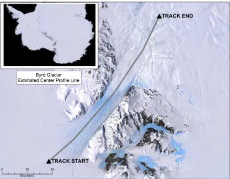
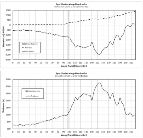
The primary research contribution presented here is ice surface, ice thickness, and 10

bed profiles along the centerlines of Byrd Glacier and Jakobshavn Isbrae, profiles ex-tracted from gridded radar-sounding flights in the map plane for these ice streams and for ice converging on these ice streams. We then use measured ice thicknesses to determine the strength of ice-bed coupling for slow sheet flow, fast stream flow, and buttressing shelf flow, thereby obtaining holistic transitions between these flow regimes. 15

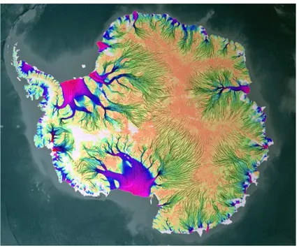
Figure 1 illustrates the challenge we faced. It is a dynamic map of ice-stream tribu-taries draining the Antarctic ice sheet and converging on major ice streams to supply large buttressing ice shelves (Rignot et al., 2011). What has been called “slow sheet flow” in the interior is better described as tributaries of faster flow imbedded in an overall regime of slower flow. This pattern invites the assumption that a thawed bed 20

predominates along tributaries and a frozen bed predominates between tributaries. “Fast stream flow” is seen as spanning a broad spectrum of ice streams having vari-ous sizes and shapes that discharge at least 90 % of Antarctic ice. “Buttressing shelf flow” occurs along margins of the largely marine West Antarctic Ice Sheet, and marine portions of the East Antarctic Ice Sheet. We treat these three flow regimes separately, 25

and then combine them holistically to quantify the Jakobshavn Effect applied to Byrd Glacier in Antarctica and to Jakobshavn Isbrae in Greenland. Summer melting on Byrd Glacier is insufficient to reach the bed to uncouple it from basal ice, and the Ross Ice Shelf buttressing Byrd Glacier is unlikely to disintegrate rapidly. Neither of these

(6)

TCD

8, 2043–2118, 2014

T. Hughes et al.

Title Page

Tables Figures

◭ ◮

Back Close

Full Screen / Esc

P

a

per

|

D

iscussion

P

a

per

|

Discussion

P

a

per

|

Discuss

ion

P

a

per

|

straints exists for Jakobshavn Isbrae. These considerations guided the conclusions we reached.

2 Ice-bed uncoupling for sheet flow

Ice-bed uncoupling begins with slow sheet flow from interior ice divides that converges on fast stream flow that supplies buttressing ice shelves. The strength of ice-bed cou-5

pling determines the first-order ice elevation above the bed. Uncoupling for slow sheet flow begins when a frozen bed thaws. A frozen bed is expected for thin ice along in-terior ice divides above subglacial highlands. Tributaries should then begin as thawed patches that gradually become linked as ice flows over a largely frozen bed. A thawed bed is expected for thick ice when the ice divide is above a subglacial basin. In this 10

case, tributaries develop over a largely thawed bed. Rignot et al. (2011) take velocities over 50 m a−1 as distinguishing faster tributaries imbedded in slower sheet flow. We use thawed fractionf of the bed to quantify ice-bed uncoupling for sheet flow along ice flowlines, withf ≥0.6 for tributaries andf ≤0.4 between tributaries, assuming thawed parts of the bed are connected along flow whenf >0.5 and disconnected forf <0.5 to 15

account for the 50 m a−1difference. An earlier approach assumed a mosaic of thawed and frozen patches, withf =1 in thawed patches and f =0 in frozen patches to map thawed, freezing, melting, and frozen zones on the bed (Denton and Hughes, 1981, Chapter 5; Hughes, 1998, Chapters 3, 5, and 9; Wilch and Hughes, 2000; Hughes, 2012, Chapter 24). Ice flow toward Byrd Glacier begins at an ice divide connecting 20

Dome Argus, where thin ice overlies Gamburtsev Subglacial Mountains and probably has a frozen bed, to Dome Circe, where thick ice overlies Wilkes Subglacial Basin and a thawed bed is possible (Drewry, 1983). We selected a flowline beginning at Dome Argus. Since tributaries converge on ice streams, flow from Dome Argus would then cross a melting bed characterized byf in the map plane gradually increasing fromf =0 25

under Dome Argus tof =1 at the head of Byrd Glacier, see Fig. 1. Sheet flow of ice to

(7)

TCD

8, 2043–2118, 2014

T. Hughes et al.

Title Page

Tables Figures

◭ ◮

Back Close

Full Screen / Esc

Discussion

P

a

per

|

D

iscussion

P

a

per

|

Discussion

P

a

per

|

Discuss

ion

P

a

per

|

Jakobshavn Isbrae also probably crosses a melting bed, since it begins at an interior ice dome where ice is frozen to the bed (Gow et al., 1997).

We treated sheet flow along ice flowlines in the downslope direction normal to ice elevation contour lines. In the simplest treatment, the force balance along a flowline balances gravitational force 1/2P_Ih_Iagainst basal drag forceτ_Oxat horizontal distance 5

x from the ice-sheet margin for basal shear stressτO, where 1/2PI=1/2ρIghI is the

average ice pressure in ice of heighthIabove the bed for gravity accelerationgand ice

densityρI. Balancing forces gives a parabolic surface profile above a horizontal bed for

constantτOas a first-order approximation (Nye, 1952a):

x=1/2(ρIg/τO)h2_I (1)

10

Actually,τO and bed topography vary alongx. These variations are included by diff

er-entiating Eq. (1) and solving for surface slopeα=dh/dx=τO/ρIghIwhen ice elevation ha.s.l. differs from ice elevation h_I above the bed, and replacing dh/dx with change ∆hin constant incremental length∆xbetween stepsi andi+l:

15

hi+l=hi+[(τO/hI)i/ρIg]∆x=[τO/(h−hB)]i∆x/ρIg (2)

whereτO andhI are specified at each∆x step for integersi. Equation (2) allows

vari-ableτO and bed topography hB=h−hI above (+) and below (−) sea level along the

flowline, which we measured by radar sounding for Byrd Glacier and Jakobshavn Is-20

brae. The bed is approximated by an up-down staircase, with α=(hi+1−hi)/∆x=

∆h/∆x= ∆hI/∆x on steps and changes±hB put between steps. When terrestrial ice

margins are on broad rather flat plains, Eq. (1) can be used to obtain height h_O at distancex from the ice margin wherei =0 in Eq. (2).

Equation (2) is an initial-value, finite-difference recursive formula. Initial ice elevation 25

h_Oabove the bed must be specified ati =0 in order to start the boot-strapping process of calculatinghI=h−hBalong the flowline at eachi step. Present-day values ofhBcan

be adjusted to account for isostatic depression and rebound of the bed during a glacia-tion cycle (Hughes, 1998, Chapter 5; Hughes, 2012, Chapter 22). This adjustment is not necessary in our study using only present-day conditions.

30

(8)

TCD

8, 2043–2118, 2014

T. Hughes et al.

Title Page

Tables Figures

◭ ◮

Back Close

Full Screen / Esc

P

a

per

|

D

iscussion

P

a

per

|

Discussion

P

a

per

|

Discuss

ion

P

a

per

|

Ice shearing over a frozen bed has basal shear stress τF that is higher than basal

shear stressτSfor ice sliding over a thawed bed or for shearing water-saturated till

be-tween basal ice and bedrock, owing to reduced ice-bed coupling when the bed thaws. Thawing lowers the ice surface. Thawed fractionf then gives:

τO=f τS+(1−f)τF=ρIghIα (3)

5

Expressions for τF and τS can be provided by respective flow laws and sliding laws

for ice (Denton and Hughes, 1981, Chapter 5; Hughes, 1998, Chapters 3 and 5; Hughes, 2012, Chapter 17). For sheet flow in the Antarctic Ice Sheet, 0.25≤f ≤0.75 is widespread, withf =0 common under ice domes over subglacial highlands andf =1 10

common under ice domes over subglacial basins and at the heads of ice streams en-tering deep fjords (Hughes, 1998, Chapter 3; Hughes, 2012, Chapter 24; Wilch and Hughes, 2000).

Flow and sliding laws give vertically averaged ice velocities and basal sliding veloc-ities, respectively, with the basal sliding velocity only slightly less than the ice surface 15

velocity owing to reduced basal drag on a thawed bed. These velocities are used in a mass-balance equation to calculate ice elevations above the bed along flowlines us-ing Eq. (3) for thawed fractionf to evaluateτO in Eq. (2). In original theories of basal

sliding, sliding velocity depends on melting and freezing rates of ice on the stoss and lee sides of bedrock bumps, and on high-stress creep rates around bumps (Weertman, 20

1957a), and also on an “effective” basal water pressure (Lliboutry, 1968). Till deforma-tion of West Antarctic ice streams appears to be nearly viscous, based on field mea-surements (Anandakrishnan and Alley, 1997), or nearly plastic, based on laboratory experiments (Kamb, 2001), conducted on the same till, let alone on different tills. Given ambiguities in deformation studies for glacial sliding over bedrock and till shearing be-25

tween basal ice and bedrock, we propose a different approach in this study based on using separate yield stresses for creep in ice and for basal sliding with till deformation. These ambiguities arise from the extreme variability of ice and till near the bed of West

(9)

TCD

8, 2043–2118, 2014

T. Hughes et al.

Title Page

Tables Figures

◭ ◮

Back Close

Full Screen / Esc

Discussion

P

a

per

|

D

iscussion

P

a

per

|

Discussion

P

a

per

|

Discuss

ion

P

a

per

|

Antarctic ice streams, as documented in detail for Kamb Ice Stream (formerly ice steam C) by Engelhardt and Kamb (2013).

Since till can deform near both the viscous and plastic ends of the viscoplastic creep spectrum, and presumably anywhere in between, depending on variable mineral com-positions, lithological textures, and water content, quantifying creep in till must allow 5

this range. We measured hI and α directly using radar sounding, so values of f in

Eq. (3) can be calculated using specified values ofτ_S and τ_F for given values of n in Fig. 2.

Figure 2 shows the viscoplastic creep spectrum for crystalline and composite mate-rials (Hughes, 1998, Chapter 9). The creep equation is:

10 ˙

ε=ε˙O(σ/σO)n (4)

where ˙εis the strain rate caused by applied stressσ, the plastic yield stress isσO, the

viscoplastic creep exponent isn, and ˙εO is the strain rate when σ=σO for all values

ofnover the range 1≤n≤ ∞. For viscous flow when n=1, the viscosity is η=σ/ε˙ 15

and yield stress σO=0. For plastic flow when n=∞, viscosity η=∞ when σ < σO

and η=0 when σ=σO. In between, a viscoplastic yield stress σV and a viscoplastic

viscosityηV=dσ/d ˙εmust be specified. For glacier ice,n=3 is typical. Two values of σV and ηV can be imagined, and are shown in Fig. 2. In the critical strain-rate yield

criterion, values at ˙εOareηVas the slope of the line tangent to the curve andσVis the

20

stress-intercept of the tangent line. In the critical shear-stress yield criterion,σV is the

point on the curve where stress curvature is a maximum andηVis the slope of the line

tangent to this point on the curve. These two yielding criteria were originally proposed for nucleation and propagation, respectively, of cracks leading to crevasse formation and calving of icebergs (Hughes, 1998, Chapter 8). We assume these two values for 25

till as well, before and after the ice fraction in till melts.

For ice to slide over bedrock or for till to be mobilized, sensible and latent heat must be provided to warm and melt ice that contacts bedrock or ice that cements basal till. Basal heat is provided by geothermal heat and frictional heat produced by deforming

(10)

TCD

8, 2043–2118, 2014

T. Hughes et al.

Title Page

Tables Figures

◭ ◮

Back Close

Full Screen / Esc

P

a

per

|

D

iscussion

P

a

per

|

Discussion

P

a

per

|

Discuss

ion

P

a

per

|

ice. Per unit volume of ice, frictional heat is the product of the shear stress and the shear strain rate (Paterson, 1994), so viscoplastic yield stressσVis defined by ˙εOat all

values ofnjust before melting takes place, withσV=0.667σOforn=3. After basal ice

in contact with bedrock or in ice-cemented till melts, basal sliding and till deformation become possible and are concentrated at the ice–bed interface whereuO is the ice

ve-5

locity. Then the creep rate does not depend on ˙εOand prevails because heat generated

by deforming unit area of basal ice is the product ofu_O andσ_V, withσ_V=0.386σ_O for

n=3. The energy needed to provide latent heat of melting is not required, so a lower stress and strain rate are allowed, compared to frozen-bed conditions. This, of course, is an assumption of convenience to avoid dealing with poorly known basal deformation 10

processes. It should be abandoned when these processes are fully quantified.

As an approximation for ice, σO=100 kPa is commonly taken (Paterson, 1994).

Then in Eq. (3),τF=σV=66.7 kPa for ice creeping above a frozen bed andτS=σV=

38.6 kPa for ice sliding above a thawed bed or for mobilized till. The gravitational driv-ing stress for sheet flow in the Antarctic Ice Sheet, where Eq. (3) applies if a mosaic 15

of frozen and thawed areas exists on the bed, is commonly 45 to 55 kPa (e.g., Budd et al., 1971; Drewry, 1983). These values lie between the 38.6 and 66.7 kPa limits for viscoplastic yield stress σV in Fig. 2 postulated here for temperate ice moving over

a thawed bed or till and for generally colder ice moving over a frozen bed or till, re-spectively applied to ice in tributaries and to ice between tributaries in our treatment 20

here.

Following Hughes (1998, Chapter 9), if thawing of a frozen bed begins in hollows between hills, so the bed becomes a mosaic of frozen and thawed patches, thawed patches will move up hills until the whole bed is thawed. Conversely, if a thawed bed becomes frozen first on hills, frozen patches will move into hollows until the whole 25

bed is frozen. This rolling bed topography typically developed before glaciation when fluvial processes produced a dendritic pattern of small streams supplying large rivers. Therefore, the thawed patches should lengthen in the direction of ice flow and become tributaries that supply major ice streams, as shown dramatically by Rignot et al. (2011)

(11)

TCD

8, 2043–2118, 2014

T. Hughes et al.

Title Page

Tables Figures

◭ ◮

Back Close

Full Screen / Esc

Discussion

P

a

per

|

D

iscussion

P

a

per

|

Discussion

P

a

per

|

Discuss

ion

P

a

per

|

for the Antarctic Ice Sheet, see Fig. 1. Their results are consistent with this way of linking thawed areas to bed topography and even subglacial lakes in applying Eq. (3), see Wilch and Hughes (2000), Siegert (2001), and Smith et al. (2009). This linkage provides the means for converting slow sheet flow into fast stream flow.

Gravitational spreading during sheet flow is resisted primarily by basal drag, so the 5

dominant resisting stress σ_xz produces strain rate ˙ε_xz=∂u_x/∂z for ice velocity u_x

when x is horizontal distance in the downslope direction of ice flow and z is vertical distance above the bed. The flow law of ice for this case is (Glen, 1958):

˙

εxz=ε˙O(σxz/σO)n=(σxz/A)n (5)

10

whereA=σO/ε˙ 1/n

O is an ice hardness parameter that depends on the fabric of

poly-crystalline ice and ice temperature. Basal drag produces an easy-glide ice fabric in ice near the bed in which the optic axes of ice crystals tend to be normal to the bed, and produces frictional heat that makes ice warmer toward the bed.

Following Hughes (2012; Appendix O), for constantAthe vertical profile of horizontal 15

ice velocity is obtained by integrating Eq. (5):

ux=2(ρIgα/A)n

h

hn_I+1−(hI−z)n+1

i

/(n+1) (6)

for which the vertically averaged horizontal ice velocity is:

ux=[2hI/(n+2)](ρIghIα/A)n=[2hI/(n+2)](τO/A)n (7)

20

Then the ratio ofuxtouxatz=hIis (n+1)/(n+2), which is 2/3 forn=1, 4/5 forn=3,

and 51/52 forn=50. Since A is kept constant, the reduction ofA near the bed due to development of an easy-glide ice fabric and the increase of ice temperature must be represented by an increase in ngreater than n=3 commonly obtained for creep 25

experiments on ice samples using stresses of about one bar (100 kPa) typical for ice

(12)

TCD

8, 2043–2118, 2014

T. Hughes et al.

Title Page

Tables Figures

◭ ◮

Back Close

Full Screen / Esc

P

a

per

|

D

iscussion

P

a

per

|

Discussion

P

a

per

|

Discuss

ion

P

a

per

|

sheets (Paterson, 1994). For ice accumulation rateaand ice thinning rater averaged alongx:

A=h4τn+1

O /(n+2)ρIg(a−r)

i1/n

(8)

The dependence of A on (a−r) quickly becomes insignificant as n increases and 5

A→τ_O. For typical flowlines 1500 km long on the East Antarctic Ice Sheet, take

ρI=917 kg m

−3

, g=9.8 m s−2, hI=3 km, α=0.002, and (a−r)=0.1 m a

−1

. Then

τO=ρIghIα=54×10 3

kg m−1s−2=54 kPa, which lies betweenτF=66.7 kPa andτS=

38.6 kPa in Eq. (3). This indicates that sheet flow occurs over a bed that is partly frozen and partly thawed to allow sliding of ice.

10

Since Rignot et al. (2011) took a surface velocity change of 50 m a−1in and between tributaries, we takeux=75 m a

−1

in tributaries andux=25 m a

−1

between tributaries for sheet flow as typical. Referring to Fig. 2, we then calculateA from Eq. (6) using

u_x at z=hI for the surface velocity when n=1 for viscous flow, n=3 for ice flow,

and n=50 for plastic flow. For u_x=75 m a−1 in tributaries, A=6.8×1013kg m−1s−1 15

whenn=1,A=4.6×107kg m−1s−2+1/3whenn₌3, andA₌7.7×104kg m−1s−2+1/50 when n=50. For u_x=25 m a−1 between tributaries, A=2.0×1014kg m−1s−1 when

n=1,A=6.7×107kg m−1s−2+1/3whenn=3, andA=7.9×104kg m−1s−2+1/50when

n=50. For both values of ux, A≈1.4×10 14

kg m−1s−1=1.4×1015 poise for n=1,

A≈5.6×107kg m−1s−5/3 for n=3, and A≈7.8×104kg m−1s−2+1/n=40 kPa when 20

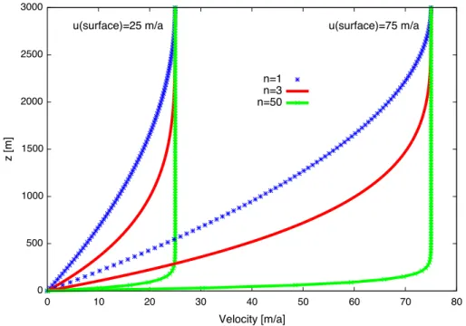
n≥50. Velocity profiles of u_x vs. z for these three values of A are plotted in Fig. 3 from Eq. (6). As n increases, A is increasingly independent of n, with u_x becoming almost constant throughhIexcept very near the bed, anduxgets closer to the surface

velocity, all signifying increasing ice-bed uncoupling. Forn >50, ice velocity becomes virtually constant throughhIasnincreases, with velocity increases confined to ice

slid-25

ing over wet deforming till at the bed. This is the condition for a thawed bed, and occurs in ice tributaries.

(13)

TCD

8, 2043–2118, 2014

T. Hughes et al.

Title Page

Tables Figures

◭ ◮

Back Close

Full Screen / Esc

Discussion

P

a

per

|

D

iscussion

P

a

per

|

Discussion

P

a

per

|

Discuss

ion

P

a

per

|

In Fig. 3, the velocity profile for n=50 is nearly linear close to the bed where a till layer may exist. A linear profile for till is obtained by setting ˙εxz=dux/dz andσxz=τV

in Eq. (5). Thenu_x=(τV/A) n

z for constantτVandAin the till layer for allnvalues.

We could use any value of n in Fig. 2 and the corresponding values of τS and τF to calculate f in Eq. (3). However, values of τO obtained from our measured

val-5

ues of hI and α using radar sounding are most compatible with τS=38.6 kPa and τ_F=66.7 kPa forn=3. This means our value ofAcalculated from Eq. (8) is vertically averaged throughhI. We could use separate values ofnfor thawed (n >50) and frozen

(3< n <50) beds forf =1 in tributaries andf =0 between tributaries, and use the cor-responding values ofA, but the choice would be arbitrary, and makes Eq. (3) useless. 10

Figure 1 then becomes a map of places wheref =1 (tributaries) and f =0 (between tributaries), which may be approximately the case, but isolated thawed patches can exist between tributaries.

It should be mentioned thatn >50 might apply if ice flows over a rugged bed consist-ing of riegels on a scale of 100 m or so. Rowden-Rich and Wilson (1996) maintained 15

that the an ice sheet would then produce its own smooth bed by developing a zone of intense shear over the tops of riegels, and applied that concept to flow from Law Ice Dome in East Antarctica. The complex pattern of tributaries in Fig. 1 would seem to preclude that possibility. However, it emphasizes the need to measure velocity pro-files in the field. Our study would benefit greatly if we had such data for Byrd Glacier 20

and Jakobshavn Isbrae in our treatment of stream flow, where that mechanism is more probable.

3 Ice-bed uncoupling for stream flow

Ice streams develop from their tributaries when basal meltwater progressively drowns bedrock bumps that penetrate basal ice and supersaturates till in directions of ice flow. 25

This occurs whenf =1, so additional melting must thicken the basal water layer, rather than increase its areal extent, and must supersaturate subglacial till. Then floating

(14)

TCD

8, 2043–2118, 2014

T. Hughes et al.

Title Page

Tables Figures

◭ ◮

Back Close

Full Screen / Esc

P

a

per

|

D

iscussion

P

a

per

|

Discussion

P

a

per

|

Discuss

ion

P

a

per

|

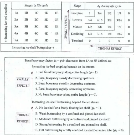
tion ϕ replaces thawed fraction f along flowlines. A geometrical force balance com-bines with a simple mass balance to calculatehI based on the formula (Hughes et al.,

2011; Hughes, 2012, Chapter 10):

ϕ=hF/hI (9)

5

wherehF is the height (thickness) of ice that floats in water. It is related to basal ice

areaAF that floats in given basal area AO so that ϕ=AF/AO becausehF is adjusted

untilhFAO=hIAF are volumes of ice that exert the same vertical gravitational force on

the bed. At a point having zero basal area, heighthF is still determined by AF/AO in

the immediately surrounding basal area, see Fig. 4. This condition exists under West 10

Antarctic ice streams (Fricker and Scambos, 2009; Engelhardt and Kamb, 2013). A holistic ice-sheet model must provide smooth transitions from sheet flow to stream flow to shelf flow for the longitudinal force balance in the direction of gravitational flow of ice, a task now accomplished by continuum models (e.g., Pattyn, 2003; Sargent, 2009; Sargent and Fastook, 2010; Blatter et al., 2011). If this force balance is done for 15

flowbands having the width of an ice stream, assumed to be constant, the six resist-ing stresses in the equilibrium equations reduce to four, a longitudinal tension stress

σT that pulls upslope ice, a longitudinal compression stressσCthat pushes downslope

ice, a basal shear stressτO due to basal drag, and a side shear stressτSdue to side

drag. Transverse stresses caused by converging and diverging flow that changes the 20

flowband width can then be ignored in the essentially one-dimensional solutions pre-sented here. This allows a force balance based on simple geometry in the longitudinal direction of ice flow, along which all of these stresses vary with changing floating frac-tion ϕ of ice in the flowband. This is a visual approach, with forces represented by geometrical areas. Partial differential equations such as the equilibrium equations are 25

avoided. For sheet flow,ϕ=0 when the bed is dry (frozen) andϕ→0 when the bed is wet (thawed). For stream flow, 0< ϕ <1 withϕ often increasing downstream. For shelf flow,ϕ=1 for a freely-floating ice shelf andϕ→1 when a confined and locally pinned ice shelf buttresses the ice stream.

(15)

TCD

8, 2043–2118, 2014

T. Hughes et al.

Title Page

Tables Figures

◭ ◮

Back Close

Full Screen / Esc

Discussion

P

a

per

|

D

iscussion

P

a

per

|

Discussion

P

a

per

|

Discuss

ion

P

a

per

|

Figure 4 is a cartoon showing places whereϕ=0 for ice grounded on a wet bed un-der an ice stream, andϕ=1 for places where ice floats in water under the ice stream. Hughes (2012, Chapter 10) assumed these places generally correspond to hills and hollows in bedrock topography, or to soft sediments or till that are unsaturated and supersaturated with water, respectively. Bedrock hills and unsaturated till resist gravi-5

tational motion. Taking Cartesian coordinates withx horizontal and positive against ice flow, y horizontal and transverse to ice flow, and z vertical and positive a.s.l., at dis-tancexfrom the ice-shelf grounding line, a flowband of widthwI has floating segments

that add up to widthwF< wI in the ice stream. Floating fractionϕdefined by Eq. (9) is

linked to the horizontal longitudinal force-and-mass balance atxusing this elaboration: 10

ϕ=w_wF

I = hF

hI

=(ρW/ρI)hW

hI

=ρWghW

ρIghI

=P

∗

W PI

(10)

whereh_F=h_I (w_F/w_I)=h_Iϕis the part of ice thicknessh_I supported by basal water,

ρW is water density, ρI is ice density, hW is an effective water depth that would float

thicknesshF of ice,P

∗

W is an effective basal water pressure that is caused by hW and

15

increases as basal drag resisting ice flow decreases, PI is the ice overburden

pres-sure, andgis gravity acceleration. In a vertical force balance, apply Newton’s second and third laws of motion to the base of columns having basal areaAO=wI∆x.

Grav-ity forces ρIghIAO and ρWghWAO are balanced by pressure forces PIAO and PWAO,

respectively, givingPW=ρWghW as the actual basal water pressure andPI=ρIghI as

20

the basal ice pressure. For ice shelves,PW=PI everywhere. For ice streams PW≈PI

because basal water flowing from sources to sinks causes variations inPW that do not

coincide everywhere withPI. TakingσWhI=P

∗

WhW in a longitudinal force balance

intro-duces back-stressσWin ice due toP

∗

W=1/2P

∗

W that resists ice motion, whereP

∗

W< PW

atx >0 under an ice stream andP∗

W=PW atx=0 under an ice shelf, see Fig. 5. At the

25

calving front water is in direct contact with a vertical ice cliffandσW=1/2PW(hW/hI) in

the longitudinal force balance.

(16)

TCD

8, 2043–2118, 2014

T. Hughes et al.

Title Page

Tables Figures

◭ ◮

Back Close

Full Screen / Esc

P

a

per

|

D

iscussion

P

a

per

|

Discussion

P

a

per

|

Discuss

ion

P

a

per

|

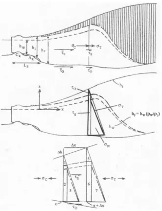
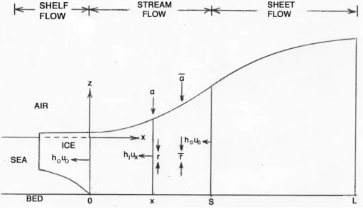
Figure 5 shows an exaggerated vertical longitudinal cross-section of a flowband from the ice divide to an ice stream and ending at the calving front of a confined and pinned ice shelf. Flow is from right to left. The top panel shows in shading the part of the flowband that rests on the bed. Solid, broken, and dashed lines show respective heights

hI,hF, andhW above basal ice. The ice shelf lies in a confining embayment grounded

5

along side lengthsLS, at an ice rise of circumference CR, and at ice rumples of area A_R, so it buttresses the ice stream. Stresses resisting gravitational flow areσ_T,σ_C,τ_O, andτS shown at distancex from the ice-shelf grounding line, andτO andτSaveraged

over the distance from 0 tox.

The middle panel shows a large triangular area equal to gravitational driving force 10

1/2PIhI. Within that triangle are areas linked to resisting forces, with the area inside the

bold border linked to compressive forceσChI and the remaining small triangular area

linked to tensile forceσThI. This force balance gives:

1/2PI=PI=σC+σT (11)

15

Note thatσC≫σTbecause area 1+2+3 enclosed by the bold border greatly exceeds

triangle area 4, so a minor downslope decrease in resistance to ice flow causes a small decrease inσCbut a large increase inσT becausePIis initially unchanged. This shows

how σT can pull more ice out of ice sheets for only a small decrease in downslope

resistance to ice flow (Hughes, 1992). 20

The bottom panel equates areas 1, 2, and 3 with compressive forceσChI, triangular

area 4 to tensile forceσThI, triangular area 3 to water-buttressing forceσWhI, area 3+4

to flotation forceσFhI, the difference between triangular areas 5 and 4 to basal drag

forceτO∆x, and the difference between rectangular areas 6 and 2 to side drag force

2τS∆x for two sides. Balancing these longitudinal forces as ∆x→0 gives (Hughes,

25

2009; Hughes, 2012, Appendix G):

σT=1/2ρIghI(1−ρI/ρW)ϕ2=PI(1−ρI/ρW)ϕ2 (12)

σC=1/2ρIghI

h

1−(1−ρ_I/ρ_W)ϕ2i=PI

h

1−(1−ρ_I/ρ_W)ϕ2i (13)

(17)

TCD

8, 2043–2118, 2014

T. Hughes et al.

Title Page

Tables Figures

◭ ◮

Back Close

Full Screen / Esc

Discussion

P

a

per

|

D

iscussion

P

a

per

|

Discussion

P

a

per

|

Discuss

ion

P

a

per

|

σW=1/2ρIghI(ρI/ρW)ϕ2=PI(ρI/ρW)ϕ2 (14)

σF=σT+σW=PIϕ2 (15)

τO=1/2ρIghI(1−ϕ)

αI−∂(hIϕ)/∂x

=PI(1−ϕ)2α (16)

τS=2ρIghI(wI/hI)

ϕαI−(1−2ϕ)∂(hIϕ)/∂x

→P_I(wI/hI)ϕ(1−ϕ)α (17)

∂(σFhI)/∂x=∂(σThI)/∂x+∂(σWhI)/∂x=PI(ρI/ρW)ϕαW (18)

5

Here_∆h/∆x→αis the ice surface slope,_∆h_I/_∆x→α_Iis the ice thickness gradient, and ∆hW/∆x→αW is the gradient of basal water height giving effective basal water

pressure P∗

W resisting gravitational ice flow as ∆x→0. Water buttressing produces

back-stressσ_W=(h_W/h_I)P∗

W in ice due toP

∗

W in a longitudinal force balance. Flotation

10

stressσF in ice is due toσW+σT in the longitudinal force balanceσFhI=σWhI+σThI.

These are real stresses. They are obscured using holistic continuum mechanics in con-ventional ice-sheet models, but they visibly emerge from the geometrical force balance in the holistic ice-sheet model based on Fig. 5.

Demonstrating that hF in Eq. (9) and P

∗

W in Eq. (10) are real, and therefore σW is

15

real, has been a challenge (Hughes, 1992, 2003, 2011, 2012, Chapter 10; Hughes et al., 2011). Relating hF to hI and hW at the calving front of an ice shelf uses the

horizontal longitudinal force balanceρIhI=ρWhWbecause heavier water of height hW

buttresses lighter ice of height hI, so hF=hI=(ρW/ρI)hW. That this is also true at

an ice-shelf grounding line is not so obvious, the objection being that ice of reduced 20

thickness buttresses ice on the forward side of an ice column to produce a concave ice-thickness profile first calculated by Sanderson (1979), then by van der Veen (1983). A rigorous force balance includes buttressing from the wedge of water under the ice column anywhere between the calving front and the grounding line (Hughes, 2012, Chapter 9). Apart from this rigorous force balance, an obvious demonstration is to melt 25

the ice shelf so water buttresses ice at the grounding line just as it did at the calving front.

(18)

TCD

8, 2043–2118, 2014

T. Hughes et al.

Title Page

Tables Figures

◭ ◮

Back Close

Full Screen / Esc

P

a

per

|

D

iscussion

P

a

per

|

Discussion

P

a

per

|

Discuss

ion

P

a

per

|

Having overcome that objection for the grounding line, the objection is still maintained that it cannot apply up an ice stream that also has a concave profile (G. Robin, personal communication, 1988; D. Pollard, personal communication, 2007). How canhWin Fig. 5

“buttress” an ice stream at distancexupstream from the ice-shelf grounding line when there is no water of heighthW atx? This confuses the distinction between a vertical

5

force balance and a longitudinal (horizontal) force balance. HeighthW acts like water

impounded by a “dam” that exists because downstream resistance to water flowing under an ice stream exists. It is similar to resistance from a laterally confined and locally pinned ice shelf that causeshW to be greater and gradient ∂hW/∂x to be less

at the grounding line than they would be for a freely-floating ice shelf. The “obvious” 10

demonstration of this is the height of water in boreholes drilled by Barclay Kamb and Hermann Engelhardt along Whillans Ice Stream: the water height above the bed was well a.s.l. and somewhat below the height needed to float ice thickness hI, so hF< hI as shown in Fig. 5, see Kamb (2001). However it is not “obvious” this validates

Eq. (10). Mean effective water pressure P∗

W “buttresses” ice in the longitudinal force

15

balance that produces a “water” back-stress σW in ice of height hI above the bed.

MacAyeal (1989) modeled Whillans Ice Stream as a linear ice shelf with some basal drag. His analytical force balance is not so different conceptually from the geometrical force balance introduced for ice streams by Hughes (1992) and illustrated in Fig. 5, where the analytical flaws are avoided by using geometry.

20

The distinction betweenP_W∗ in Eq. (10) andPWis thatPW≈PIvertically when the bed

is wet, butP_W∗ < PI horizontally in proportion toAW< AOfor ice floating over basal area AF=AW within basal areaAO. Where Kamb and Engelhardt drilled through Whillans

Ice Stream,A_W wasn’t much less thanA_O.

The longitudinal force balance pits gravitational driving force gradient∆(PIhI)/∆x=

25

P_Iα as ∆x→0, obtained from the difference between area 5+6+7+8 and area 1+ 2+3+4 in incremental length∆x in Fig. 5, against resisting stresses τO and τS and

(19)

TCD

8, 2043–2118, 2014

T. Hughes et al.

Title Page

Tables Figures

◭ ◮

Back Close

Full Screen / Esc

Discussion

P

a

per

|

D

iscussion

P

a

per

|

Discussion

P

a

per

|

Discuss

ion

P

a

per

|

flotation force gradient∂(σFhI)/∂xto obtain (Hughes, 2011, 2012, Appendix G):

PIα=τO+2τS(hI/hW)+∂(σFhI)/∂x (19)

Equation (19) is satisfied using substitutions from Eqs. (16)–(18).

Now approximate bed topography with an up-down staircase in which∆xis the con-5

stant step length and±_∆h_B is the variable gain or loss in step height. A normal stress

σ_Nin the direction of ice flow pushes against−∆h_Band pulls away from+∆h_Bwith force

FN=±σN∆hBcompared to gravitational driving forceFG=PIhI, so thatσN∆hB/∆xand PI∆h/∆x are force gradients with σN close to viscoplastic yield stress σV in Fig. 2.

ThenFN is much less than FG until the bed slope exceeds ±30

◦

(Hughes, 2012, Ap-10

pendix E), soFN can be ignored for lesser bed slopes. Then ∆h= ∆hI can be used

for each ∆x step. Substituting Eqs. (16)–(18) into Eq. (19), putting terms containing

∂ϕ/∂xbetween∆x steps, dividing byPI, solving for surface slopeα, and returning to

the incremental form so∂ϕ/∂x≈_∆ϕ/_∆x andα≈_∆h/_∆x:

∆h

∆x =

∆(σFhI)/∆x PI

+τO

PI

−2τS(hI/hW)

PI

(20) 15

=ϕ2

∆hI

∆x

F

+(1−ϕ)2

∆hI

∆x

G

+2ϕ(1−ϕ)

∆h

∆x

Here∆hI= ∆hon∆x steps, so (∆h/∆x)F is for the floating fraction of the ice column

linked toσ_Fand (∆h/∆x)_G is for the grounded fraction of the ice column linked toτ_Oon these steps. Putting∆hB/∆x and∆ϕ/∆x between∆x steps is a major simplification

20

that avoids integrating partial differential equations. If unwarranted, this assumption invalidates everything that follows, see Hughes (2012, Chapter 20, Appendices E and P).

When only the geometrical force balance is used, Eq. (9) becomes (Hughes, 2012, Chapter 11):

25

ϕ=hO/hI (21)

(20)

TCD

8, 2043–2118, 2014

T. Hughes et al.

Title Page

Tables Figures

◭ ◮

Back Close

Full Screen / Esc

P

a

per

|

D

iscussion

P

a

per

|

Discussion

P

a

per

|

Discuss

ion

P

a

per

|

Equation (21) is obtained both for ice streams with side shear and for the central flow-line of an ice stream without side shear. In Eq. (21), hO is ice height above the bed

atx=0 where the ice stream becomes a floating ice shelf, sohO=hIwhenϕ=1 but ϕ <1 at horizontal distancesx up the ice stream wherehO< hI. For sheet flow,ϕ=0

5

becausehO=0 at the ice margin. For shelf flow,ϕ=1 whenhO=hI everywhere. For

stream flow, 1> ϕ >0 becausehI> hO. The mass balance must be combined with the

force balance to obtain solutions ofϕthat satisfy Eq. (9).

A simple mass balance is shown in Fig. 6 for constant ice accumulation rateaand ice thinning rater alongx, withhI=hL where ice velocityux=0 at the ice divide (x=L),

10

hI=hS whereux=uS and stream flow begins (x=S), andhI=hO whereux=uO at

the ice-shelf grounding line (x=0), so that:

(a−r)(L−x)=hIux (22)

Sinceaandr can vary alongx, Eq. (22) is a simplification comparable to Eq. (20) and, 15

if unwarranted, invalidates everything that follows. Validation requires thatϕ,h_B,a, and

r vary slowly along x.

Here is how (∆h/∆x)G is obtained. Assume the bed is thawed in grounded areas AG=AO−AFso grounded ice slides over the bed at velocityuS. Using a conventional

sliding law for ice (Weertman, 1957a), whereBincludes bed roughness and physical 20

properties of temperate ice at the bed,m=2 for sliding ice, andu=u_x=uS:

u=uS=

_τ

O B

m

(23)

Equate ice elevationhwith ice thicknesshI for a horizontal bed at sea level. Combine

Eqs. (22) and (23), withτO=ρIghIdhI/dx now depending only on the strength of

ice-25

bed coupling linked to grounded thawed fractionf =1 under ice streams:

(21)

TCD

8, 2043–2118, 2014

T. Hughes et al.

Title Page

Tables Figures

◭ ◮

Back Close

Full Screen / Esc

Discussion

P

a

per

|

D

iscussion

P

a

per

|

Discussion

P

a

per

|

Discuss

ion

P

a

per

|

Now lethIvary with bed topography, using measured values ofhI in Eq. (24). Solve for

surface slopeα=dh/dx:

α=dh dx =

B ρIghI

(a−r)(L−x)

hI

_m1

(25) 5

TakingτO=ρIghIα and setting α=(∆h/∆x)G for ice grounded in incremental length

∆x, Eq. (25) gives:

∆hI

∆x

G

= τO

ρIghI

=(B/ρIg)[(a−r)(L−x)]

1 m

hmm+1 I

(26)

Note the weak dependenceh_I∝(a−r)1/3form=2. To a first approximation, this “justi-10

fies” ignoring slow variations of (a−r) and also ofaandr separately alongxin Eq. (22). Calculating (∆h/∆x)F begins with the mass balance in Fig. 6 written as follows:

hIux=hOuO+(a−r)x (27)

Note that velocitiesu_x and uO are negative with x positive upslope. Differentiating at

15

pointx:

∂(hIux)/∂x=∂[hOuO+(a−r)x]/∂x=(a−r) (28)

=u_x∂hI/∂x+hI∂ux/∂x=ux∂hI/∂x+hIε˙xx

where ˙ε_xx=∂u_x/∂x is the longitudinal strain rate alongx. Solve for incremental slope 20

(∆h/∆x)_F by settingux=uand ˙εxx=ε˙ withuxobtained from Eq. (24):

∆h

∆x

F

=(a−r_u)−hIε˙

x =

hI(a−r)−h 2 Iε˙ hOuO+(a−r)x

(29)

(22)

TCD

8, 2043–2118, 2014

T. Hughes et al.

Title Page Abstract Introduction Conclusions References Tables Figures ◭ ◮ ◭ ◮ Back Close

Full Screen / Esc

Printer-friendly Version Interactive Discussion P a per | D iscussion P a per | Discussion P a per | Discuss ion P a per |

Using the flow law of ice (Glen, 1958), whereAis an ice-hardness parameter depen-dant on temperature and n=3 for ice, ˙εxx= ∆u/∆x is the extending strain rate for

stressσT given by Eq. (12) withϕ=1 for floating ice, andR is a dimensionless scalar

that takes account of other strain rates in addition to ˙ε_xx: 5

˙

ε=ε˙xx= ∆u/∆x=R σ′ xx A !n =R _σ T 2A n (30)

where deviator stressσxx′ =1/2σT for ice streams (Hughes, 2012, Chapter 10). From

Hughes (2012, Appendix A):

R= 

1+ ˙

ε_yy

˙

ε_xx

!

+ ε˙yy ˙

ε_xx

!2

+ ε˙xy ˙ ε_xx !2 + _ε_˙ xz ˙ ε_xx 2  

n−1

2

(31) 10

Here ˙εxx, ˙εyy, ˙εxy and ˙εxz are strain rates associated with longitudinal extension,

lat-eral compression, side drag, and basal drag, respectively. Latlat-eral compression occurs when slow sheet flow converges on fast stream flow, but ice streams have relatively constant widths. There is no lateral shear down the centerline of ice streams, and 15

there is little basal shear if the bed is wet andϕis high. So ˙ε_xx is the dominant strain rate andR≈1 forn=3 is a useful approximation. However, ˙ε_xy cannot be ignored for narrow ice streams (Dupont and Alley, 2005a, b). For the central flowline of a narrow ice stream, the contribution from ˙ε_xy can be added to ˙ε_xz.

Collecting terms in Eq. (20): 20

(1−2ϕ+2ϕ2)∆h/∆x=ϕ2

∆h

∆x

F

+(1−ϕ)2 ∆h ∆x G (32)

Writing as a quadratic equation:

(23)

TCD

8, 2043–2118, 2014

T. Hughes et al.

Title Page Abstract Introduction Conclusions References Tables Figures ◭ ◮ ◭ ◮ Back Close

Full Screen / Esc

Printer-friendly Version Interactive Discussion Discussion P a per | D iscussion P a per | Discussion P a per | Discuss ion P a per | + ∆h ∆x − ∆h ∆x G =0

SettingC1=(∆h/∆x),C2=(∆h/∆x)F, andC3=(∆h/∆x)Gand solving forϕgives the

solution for an ice stream having constant width and side shear:

ϕ=

(C1−C3)±

h

(C1−C3) 2

−(C₁−C₃)(2C₁−C₂−C₃) i1₂

(2C1−C2−C3)

(34) 5

In a flowline solution, widthwI=0 soτS=0. Yet side drag remains and contributes to

the ice elevation needed to overcome resistance to ice flow, so it must be taken into account in some way, especially for narrow ice streams (Dupont and Alley, 2005a, b). The best way is to enlargeτO to effective basal shear stressτ

∗

O linked to areas 5+6

10

minus areas 1+2 as incremental length∆x→0 in Fig. 5. Thenτ∗

Ois:

τ∗

O=ρIghI(1−ϕ2)∆h/∆x−ρIgh2Iϕ∆ϕ/∆x (35)

and the longitudinal force balance, putting the∆ϕ/∆x terms in Eqs. (16) through (18) between_∆xsteps, becomes (Hughes, 2012, Chapter 11):

15 ∆h

∆x =

∆(ρFhI)/∆x PI

+τ

∗

O PI

=ϕ2

∆h

∆x

F

+(1−ϕ2) ∆h ∆x G (36)

Collecting terms containingϕgives:

∆h

∆xG

−

∆h

∆xF

ϕ2−

∆h

∆xG

− ∆h ∆x

=0 (37)

20

Solving forϕgives the solution for an ice-stream centerline with side shear added to basal shear:

ϕ=± _C

3−C1 C3−C2

1₂

(38)

(24)

TCD

8, 2043–2118, 2014

T. Hughes et al.

Title Page

Tables Figures

◭ ◮

Back Close

Full Screen / Esc

P

a

per

|

D

iscussion

P

a

per

|

Discussion

P

a

per

|

Discuss

ion

P

a

per

|

In Eqs. (34) and (38), the correct solution putsϕin the range 0≤ϕ≤1.

Equation (33) includes (∆h/∆x)F for floating fractionϕof ice in our model, linked to

longitudinal strain rate ˙ε_xx as seen in Eq. (29), and also to the flow law of ice given by Eq. (30) which links ˙ε=ε˙_xz toσ_T given by Eq. (12). The longitudinal strain rate is 5

therefore, using Eq. (12) forσTand following Hughes (2012, Chapter 12):

˙

ε=ε˙xx=(σT/2A)n=

h

(ρIghI/4A)(1−ρI/ρW)ϕ2

in

(39)

=[(ρIghI/4A)(1−ρI/ρW)−(σB/2A)]n

Here σB is a back-stress due to buttressing by a confined and pinned ice shelf given

10 by:

σB=fB

1