www.clim-past.net/10/825/2014/ doi:10.5194/cp-10-825-2014
© Author(s) 2014. CC Attribution 3.0 License.
Climate
of the Past
A probabilistic model of chronological errors in layer-counted
climate proxies: applications to annually banded coral archives
M. Comboul1, J. Emile-Geay1, M. N. Evans2, N. Mirnateghi1, K. M. Cobb3, and D. M. Thompson4
1Department of Earth Sciences, University of Southern California, 3651 Trousdale Parkway, ZHS 275, Los Angeles,
California 90089, USA
2Department of Geology, University of Maryland, College Park, Maryland 20742, USA
3Department of Earth and Atmospheric Sciences, Georgia Institute of Technology, 311 Ferst Drive, Atlanta,
Georgia 30332, USA
4Department of Geosciences, University of Arizona, 1040 E. 4th Street, Tucson, Arizona 85721, USA
Correspondence to:M. Comboul ([email protected])
Received: 7 October 2013 – Published in Clim. Past Discuss.: 31 October 2013 Revised: 11 February 2014 – Accepted: 6 March 2014 – Published: 25 April 2014
Abstract. The ability to precisely date climate proxies is central to the reconstruction of past climate variations. To a degree, all climate proxies are affected by age uncertain-ties, which are seldom quantified. This article proposes a probabilistic age model for proxies based on layer-counted chronologies, and explores its use for annually banded coral archives. The model considers both missing and dou-bly counted growth increments (represented as independent processes), accommodates various assumptions about error rates, and allows one to quantify the impact of chronologi-cal uncertainties on different diagnostics of variability. In the case of a single coral record, we find that time uncertainties primarily affect high-frequency signals but also significantly bias the estimate of decadal signals. We further explore tun-ing to an independent, tree-rtun-ing-based chronology as a way to identify an optimal age model. A synthetic pseudocoral network is used as testing ground to quantify uncertainties in the estimation of spatiotemporal patterns of variability. Even for small error rates, the amplitude of multidecadal variabil-ity is systematically overestimated at the expense of interan-nual variability (El Niño–Southern Oscillation, or ENSO, in this case), artificially flattening its spectrum at periods longer than 10 years. An optimization approach to correct chrono-logical errors in coherent multivariate records is presented and validated in idealized cases, though it is found difficult to apply in practice due to the large number of solutions. We close with a discussion of possible extensions of this model and connections to existing strategies for modeling age un-certainties.
1 Introduction
A peculiar feature of the Earth sciences is that the indepen-dent variable used to peer into Earth’s past (the age of the sample) is always uncertain to some degree. In paleoclima-tology, time uncertainties depend on the record’s structure, which belongs to one of two categories:
1. Tie-point chronologies, which include most sedi-mentary and speleothem archives. Such records are dated via a one-to-one mapping between sample depth and age (that is, an age model). This model typically assumes a piecewise-continuous accumula-tion rate, constrained by a relatively small number of radiometrically determined tie points (e.g., 14C dates for sedimentary archives, or U/Th dates for speleothem archives). Alternatively, when radiomet-ric dating proves impossible, records are often dated by “tuning” to a reference chronology, either derived astronomically (orbital tuning; e.g., Bender, 2002; Hays et al., 1976; Lisiecki and Raymo, 2005; Martin-son et al., 1982) or derived from a better-constrained chronology such as the GISP2 record (Grootes et al., 1993) or the Hulu Cave chronology (Wang et al., 2001).
elapsed since the creation of the topmost (most re-cent) observed layer. Equivalently, layers may be iden-tified through observation of a seasonally or annually varying quantity such as isotopic composition (Fair-banks and Dodge, 1979). Layer-counted chronologies are assigned ages relative to a modern tie point un-less supplemented by independent age controls, such as by radiometric dating (e.g., Cobb et al., 2003; Shen et al., 2013), and often assume continuous time res-olution unless observations indicate otherwise (e.g., St. George et al., 2013).
Although records from banded archives can often reach subannual precision, they are not time certain and these un-certainties can have a large influence on variability and co-herence between the records. Tree-ring chronologies are gen-erally considered the most accurately dated, because – unlike other proxy types – they are often built from a large num-ber of records. Nonetheless, they require adjustments (cross-dating) to optimize coherence across nearby sites (e.g., Dou-glass, 1941; Fritts, 1976; Wigley et al., 1987; Cook and Kair-iukstis, 1990; Yamaguchi, 1991; Stokes and Smiley, 1996). Similarly, although the quoted uncertainty on ice core layer counting is typically on the order of 2 % (Alley et al., 1997b), this value reflects the reproducibility from one chronolo-gist to the next, not the uncertainty about the true date. Seimon (2003) thus showed how two nearby Andean ice cores (Thompson et al., 1985) differed widely when plot-ted against their published timescales, but that simple ad-justments based on volcanic tephra markers could bring the records into excellent agreement. Finally, Emile-Geay et al. (2013) showed how minor age uncertainties in several high-resolution records (in particular coral chronologies) could mute interannual signals in a multiproxy reconstruction of tropical Pacific sea surface temperature.
Time uncertainties pose a serious challenge to the anal-ysis of paleoclimate signals, as the mathematical machin-ery devoted to time series analysis (e.g., spectral analysis, singular spectrum analysis, wavelet analysis) or multivariate analysis (e.g., principal component analysis, regression anal-ysis, climate field reconstruction) implicitly assumes a per-fectly known time axis. In the non-banded case, this prob-lem was recognized early on and motivated the use of tun-ing, though this approach is not without dangers (Blaauw, 2012). Recently, several studies have chosen instead to ex-plicitly take time uncertainties into account (Huybers and Wunsch, 2004; Blaauw, 2010; Haam and Huybers, 2010; Blaauw and Christen, 2011; Rhines and Huybers, 2011; Bre-itenbach et al., 2012; Anchukaitis and Tierney, 2012), which has greatly helped quantifying the uncertainties inherent to the interpretation of climate signals in such records.
To our knowledge, banded records have not spurred sim-ilar modeling efforts, with the notable exception of Rhines and Huybers (2011), whose model targeted long ice-core chronologies like that of GISP2 (Alley et al., 1997b). Their
study used a discrete random walk, which assumes that the probability of missing a band, or counting a band twice, is symmetric. However, these probabilities are likely asymmet-ric for most proxies. Further, the model forced the authors to make some unphysical choices in order to match pub-lished estimates of age uncertainties. The model we propose is formulated more intuitively in terms of the probabilities of miscounting a band, and naturally allows for asymmetries in the probability of missing or doubly counting a band. Our work also applies the model to multivariate data sets and ex-plores ways to correct for age errors using information shared amongst similar records.
Since dendroclimatology has dealt with layer-counted chronological errors for decades, it would be tempting to draw from their extensive literature for other proxy classes. Unfortunately, extending dendrochronological techniques to other proxy types spanning large spatial scales is problem-atic, because cross-dating relies on the existence of a strong common signal shared among series. This assumption is well suited to trees within a restricted biome but may no longer be valid for other proxy types with banded age models (ice cores, annually banded corals, varved sedimentary records), either because too few (if any) replicates are available at a given site or because one is interested in synchronizing records across a wide geographical area (e.g., a pan-Pacific coral network), where the common signal may be weaker. Nevertheless, this approach was successfully applied to repli-cated coral records from the reefs offshore of Amédée Island, New Caledonia (DeLon et al., 2007; DeLong et al., 2013), and from the Gulf of Mexico (DeLong et al., 2011).
In this article we propose a new probabilistic age model for layer-counted records (Sect. 2.1) and use it to quantify the consequences of such errors in single- and multiproxy applications. Implicit in our approach is the assumption that optimal sampling strategies were utilized, so chronological errors are a leading source of uncertainty. We first use the model to quantify the uncertainty associated with spectral es-timates from univariate coral series (Sect. 2.2). We then gen-eralize this framework to the multivariate setting (Sect. 3.1), evaluating the impact of chronological uncertainties on prin-cipal component analysis derived from a pan-Pacific coral network (Sect. 3.3). Leveraging the mutual information from these signals, we then propose a method to correct for age uncertainties in banded records (Sect. 4), which we validate on synthetic data. Discussion follows in Sect. 5.
2 Banded age model: design and application
2.1 Univariate model formulation
t1=tf, whose date is assumed to be known exactly, earlier
times are deduced by assuming that observations are consec-utive (see Fig. 1), so previous observationsti,i∈ {2,· · ·, n} follow the relation
ti=ti−1−1i, (1)
where1is a vector of time increments taking integer val-ues. In this study, we do not consider records derived from multiple-year sampling intervals (Linsley et al., 2006, 2008) nor bulk averages (Hendy et al., 2002; Calvo et al., 2007), which are straightforward extensions of our model. Thus, for error-free annually banded proxies,1i=1=1 year exactly (Fig. 1a). Several sources of error, however, may perturb this ideal chronology. For instance, a coral may fail to form a band during a year of particularly poor growing conditions (related to water turbidity, excessive temperature, or other ecological factors) or years may be missing due to sampling artifacts (e.g., core breaks); a tree may fail to form an annual growth increment in an excessively dry or cold year; an ice core may miss a layer due to low deposition or high wind ablation that year; and a varved sediment core may miss a year because of low productivity in that particular year. Con-versely, a single (large) coral band, in a fast growth state, may be associated with two (multiple) consecutive years in-stead of a single one. Additionally, stress bands or changes in growth orientation (e.g., Fig. 1c) may also create “false” sec-ondary bands (see Alibert and Kinsley, 2008; DeLong et al., 2013). Thus, in reality, each entry1ican take any positive in-teger value (to preserve the layer superposition principle), al-though1i=1 most of the time. Considering that error rates are typically asymmetric (with double counting being more common than missing years; DeLong et al., 2013), we use a stochastic model (Appendix A), in which the increment vector comprises two independent stochastic processesPθ1
andPθ2, with parametersθ
1andθ2, representing the rates of
missing and doubly counted bands, respectively.
Age errors are cumulative: for a 100-year-long record, an error rate of 5 % forθ1andθ2will lead to offsets as large as ±5 years by the beginning of the sequence, with a probability of∼15 % (cf. the shifted initial dates of the perturbed signals in Fig. 2b). Although there is partial compensation between over- and undercounting, leading to a zeroexpectedoffset in the symmetric case, this expectation is misleading. Indeed, assuming the independence of age errors from one record to another, there is a roughly 2 % chance that the oldest date of each record will be offset by as many as 10 years (Eq. A7). Though such probability is low, it is non-negligible, and we shall see in Sect. 3.3 that in the case of a multivariate data set it may severely bias the estimation of spatiotemporal modes of variability, far beyond the annual scale.
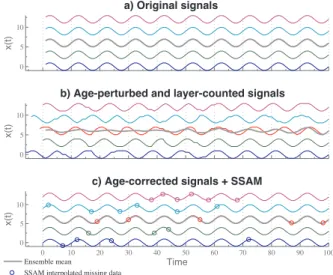
This error model may be used in two ways, as illustrated in Fig. 2 with simple sinusoidal signals:
i. Starting from an error-free chronology (Fig. 2a), one may perturb it by randomly removing or duplicating
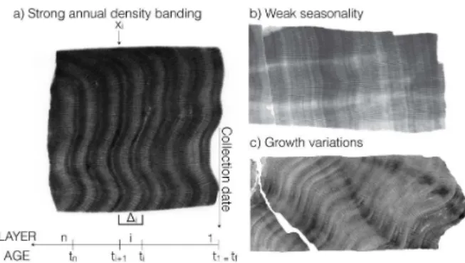
Fig. 1.Coral core X-radiographs: (a)top of a core from Mange Reef, Tanzania (Cole, unpublished). Each layer shows the chang-ing density of the coral growth over a year. Observationxi could
be theδ18O measured from theith layer (most likely correspond-ing to1i=1 year). The collection datet1and the oldest onetnare
also shown to illustrate our notation;(b)top of a core from Onotoa, Republic of Kiribati (Thompson, unpublished) showing weak sea-sonality and annual density banding;(c)Fanning Island fossil coral
V33, aged∼6500 years old (Cobb et al., 2013), with a varying
growth axis, which typically requires multiple sampling transects.
layers whenPθ1
i ≥1 orP θ2
i ≥1, and linearly reassign-ing time to the correspondreassign-ing observations (Fig. 2b). This allows one to explore the effect of age errors in idealized scenarios.
ii. Starting from a real chronology, which inevitably con-tains errors (Fig. 2b), one may use the model to gener-ate plausible corrections, given some knowledge of the miscounting rate (Fig. 2c shows the signals corrected with the true-age model). In this case, extra data entries must be inserted wherePθ1
i ≥1, while layers must be removed wherePθ2
i ≥1.
The former case requires interpolation of the data where lay-ers are believed to be missing. While linear interpolation is often used for simplicity, it tends to suppress high-frequency variability, hence potentially distorting a record’s spectrum. To preserve the intrinsic autocorrelation structure of the time series, we use singular spectrum analysis (SSA; Broomhead and King, 1986; Fraedrich, 1986; Vautard and Ghil, 1989) and its missing value counterpart (SSAM) (Schoellhamer, 2001) to reconstruct the time series including miscounted layers. SSAM was shown to preserve the variance for as many asM2 missing points within a sliding window of sizeM
0 5 10
a) Original signals
x(t)
0 5 10
b) Age-perturbed and layer-counted signals
x(t)
0 10 20 30 40 50 60 70 80 90 100
0 5 10
c) Age-corrected signals + SSAM
x(t)
Time Ensemble mean
SSAM interpolated missing data
Fig. 2.Illustration of the phase distortion of coherent signals due to miscounted annual bands withθ1=θ2=0.05 and a collection datet1=100.(a)Five hypothetical and identical harmonic signals shifted vertically for clarity;(b) the same signals after introduc-ing age perturbations and makintroduc-ing the (erroneous) assumption that 1 layer amounts to 1 year (note the loss of coherency reflected in the ensemble mean in gray, which is performed as part of composites in most climate reconstructions);(c)the same age-perturbed sig-nals, after correcting for miscounted bands and interpolating miss-ing data with SSAM.
2.2 Uncertainty quantification in coral records
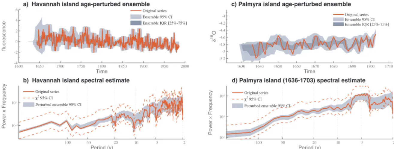
The above model is now applied to two coral data sets. The first one is the Havannah Island fluorescence record (Isdale et al., 1998), chosen for its particularly long, continuous time span. Because the record already contains dating inaccura-cies, we attempt to correct for age errors as explained in Sect. 2.1(ii). The age uncertainty in coral records is not usu-ally known, because many of them are not site-replicated. However, DeLong et al. (2013) suggested an error rate from
−2.1 to 3.7 % in unreplicated samples. Error rates may be higher at sites with weak seasonality (Fig. 1b) or in cores with varying growth structures (Fig. 1c). We thus assume a conservative error rate of 0.05 for both missing and doubly counted annual bands (i.e.,θ1=θ2=0.05) and generate an
ensemble of 1000 plausible age-corrected realizations. The 95 % confidence interval (CI) of the realization ensemble is shown along with the original time series in Fig. 3a.
The corresponding spectral densities were estimated in Fig. 3b using the multi-taper method (MTM; Thomson, 1982) for each age model realization with a conservative time-bandwidth product of 7/2 (results are insensitive to this choice).
It is generally presumed that dating errors should affect the estimation of interannual variance most strongly, but only negligibly affect decadal signals. Figure 3b shows this ex-pectation to be approximately correct, though the impact on
decadal variability is substantial. Indeed, the width of the confidence bands roughly triples from periods of 50–5 years. It is, however, noteworthy that the spectral uncertainties due to the age perturbations (shaded area) are markedly nar-rower than the uncertainties in the spectral estimates them-selves (dashed lines, obtained via standard χ2 intervals), even though a widening of the ensemble spread can be ob-served as the frequency increases. This result persists with the robust method of Chave et al. (1987) and its associated jackknife intervals.
To check that those results are not an artifact of the choice of coral time series, we repeat this analysis on aδ18O record from Palmyra Island (Cobb et al., 2003). Figure 3c shows the cold-season average (December-January-February, DJF) of a continuous splice (1636–1703) of this record, together with the width of the age-perturbed ensemble using θ1=
θ2=0.05. Figure 3d shows the impact of age uncertainties
on the estimated spectrum, and confirms the previous re-sults: spectral energy of time-uncertain data sets leaks from the interannual band to lower frequencies, but chronologi-cal uncertainties generally produce narrower intervals than those due to the spectral estimation process. Although this record was obtained from a fossil sample for which the top-most layer was U/Th dated, in this experiment we did not in-clude the U/Th dating uncertainties since no spectral defor-mation should arise from sliding the whole sequence across the U/Th error window.
2.3 Age model identification
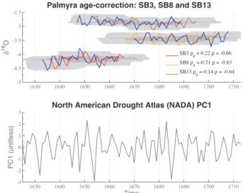
We have shown how the model described in Sect. 2.1 can be used to generate ensembles of plausible chronologies for any banded record given some a priori estimate of chronological errors. Learning from other data series with more replicated and accurate chronologies can then be used to choose an opti-mal chronology from an ensemble of plausible chronologies. For example, Li et al. (2011) adjusted age assignments of U/Th-dated fossil Palmyra Island corals, observing that the correlation between the nominally dated modern record, and the first principal component of the North American Drought Atlas (NADA PC1), interpreted as a proxy for El Niño– Southern Oscillation (ENSO)-related hydroclimatic variabil-ity, was highly significant over the 1891–1994 time period. They then used this property to align the older sequences, before the onset of the instrumental period, to NADA PC1 within the range of U/Th dating error. To identify an optimal chronology, we similarly choose the realization that maxi-mizes the correlation between the Palmyra coral record and the NADA PC1 during their periods of overlap (Fig. 4). As in Li et al. (2011), we account for the estimated±10 years U/Th dating errors by shifting the final timetf of the
en-semble of plausible chronologies generated with our model across a 21-year window, so the ensemble size is 20 times larger than in the knowntfcase. For convergence purposes,
1600 1650 1700 1750 1800 1850 1900 1950 2000 -4
-2 0 2 4 6
Time
fluorescence
a) Havannah island age-perturbed ensemble Original series Ensemble 95% CI Ensemble IQR [25%-75%]
100 50 20 10 5 2
10-2
10-1
Period (y)
Power x Frequency
b) Havannah island spectral estimate
Original series 2
95% CI
Perturbed ensemble 95% CI
1630 1640 1650 1660 1670 1680 1690 1700 1710
-5.2 -5 -4.8 -4.6 -4.4 -4.2 -4
Time
18
O
c) Palmyra island age-perturbed ensemble
Original series Ensemble 95% CI Ensemble IQR [25%-75%]
100 50 20 10 5 2
10-3
10-2
10-1
Period (y)
Power
Frequency
d) Palmyra island (1636-1703) spectral estimate
Original series 2
95% CI
Perturbed ensemble 95% CI
Fig. 3.Ensemble realization (top) and power spectra (bottom) of age-perturbed coral data for(a, b)Havannah Island (Isdale et al., 1998) and(c, d)Palmyra Islandδ18O record from 1636 to 1703 (Cobb et al., 2003), where the top layer is U/Th dated. The original data and corresponding spectral estimates are shown in red, and the 95 % confidence intervals (CIs) and the 25–75 % interquartile range (IQR) of the perturbed data ensemble and corresponding spectra are shown by the shaded areas. Power spectra are represented in variance-preserving coordinates (that is, the area under the curve is an exact measure of the variance contained in each frequency band).
error rates as in the previous section (θ1=θ2=0.05). The
selected chronologies (blue curves in the top Fig. 4) improve the correlation coefficient of the individual series to NADA PC1 by a factor of 3 relative to the published chronologies (before dating errors were corrected). Those results are com-parable to the improvement obtained in Li et al. (2011) after adjustments.
A caveat of this approach is that it assumes a perfectly known NADA PC1 chronology, whereas in reality it is also estimated from layer-counted archives. For a full appraisal of uncertainties in this synchronization process, one would ide-ally apply this approach to the NADA records as well. How-ever, the large number of cross-dated tree-ring chronologies in NADA (several thousand over this time interval) makes it likely that these uncertainties are negligible compared to those associated with coral dating.
3 Multivariate generalization
Climate proxies are increasingly used as part of large-scale data syntheses (e.g., PAGES2K Consortium, 2013; Marcott et al., 2013; Tierney et al., 2013; Tingley and Huybers, 2013). We thus generalize the previous model to the case of a multi-variate network and investigate the effect of age errors on the estimation of spatiotemporal modes of climate variability.
3.1 Model formulation
Let us consider a multivariate banded data set{ζ,τ}, with
ζ the data matrix containingnproxy measurements atp lo-cations (for instance,δ18O or Sr/Ca) andτ the time matrix. Each entryζij,(i, j )∈ {1, . . . , n} × {1, . . . , p}corresponds to
theith observation at thejth location, and is assigned a time
τij=ti(j ). At each locationj, miscounting events are
repre-sented by independent stochastic processesPθ1jandPθ2j(for
missing and double bands, respectively; see Appendix A). This formulation allows different error parametersθ1jandθ2j
for each locationj.
As in Eq. (A3), errors are cumulative and may lead to im-portant age offsets in the earlier portions of the data set. To see this, consider the situation depicted in Fig. 2, which con-siders five coherent, monochromatic signals. Age errors on these harmonic signals were simulated according to Eq. (A5), usingθ1j=θ2j=0.05. The figure illustrates how even small
age offsets introduce phase distortion that lowers the co-herency between signals, producing an apparent amplitude modulation of the periodic component, whose amplitude ap-pears to grow over time. In Sect. 4 we exploit this property to identify age models based on their ability to correct for this loss of coherency.
3.2 Pseudocoral benchmark
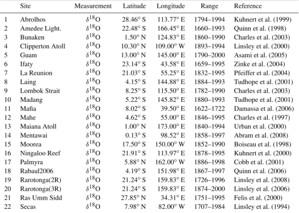
To illustrate the use of the model described above, and to val-idate our approach, we need a data set that is free of chrono-logical errors and measurement noise. We thus consider a “pseudocoral” network of 22 corals, derived from simulated climate fields. Pseudocoral locations (Table 1) were chosen to mimic the position of publicly available1 coralδ18O ob-servations with a resolution better than 2 months (Fig. 5).
The pseudocoral observationsC= {ζ,τ}were simulated according to the forward model of Thompson et al. (2011), a simple representation of the effects of temperature and sea water isotopic variation on the oxygen isotope composition of coral aragonite:
ζij=a1SSTij+a2SSSij+σ·ǫij, (2)
1630 1640 1650 1660 1670 1680 1690 1700 1710 -5
-4.5 -4 -3.5 -3 -2.5
I
18
O
Palmyra age-correction: SB3, SB8 and SB13
SB3 W
0 = 0.22 W = -0.66 SB8 W
0 =-0.21 W = -0.63 SB13 W
0 =-0.14 W = -0.64
1630 1640 1650 1660 1670 1680 1690 1700 1710
-3 -2 -1 0 1 2 3
North American Drought Atlas (NADA) PC1
PC1 (unitless)
Time
Fig. 4.Palmyra relict coralδ18O records (top): published data SB3 in red, SB8 in orange and SB13 in brown (Cobb et al., 2003); the shaded area is the 95 % confidence interval of the ensemble of re-alizations with final time shiftedtf±10 years andθ1=θ2=0.05, and the blue chronology corresponds to the realizations that maxi-mize the correlation with the first principal component of the NADA record (bottom) over each continuous section. For SB3, there were 2 added years and 2 removed years, andtfwas shifted by−2 years.
For SB8, there were 2 added years and 2 removed years, andtf
was shifted by 5 years. For SB13, there were 1 added year and 2 removed years, andtfwas shifted by−6 years. The correlation
co-efficients with NADA PC1 are also shown, whereinρis computed
using the aligned Palmyra chronologies, andρ0using the original chronologies.
wherea1anda2, locally constant coefficients, describe the
dependence of oxygen isotopic equilibrium on the tempera-ture of carbonate formation and the regional relationship be-tween SSS and sea waterδ18O, respectively.ǫ∼N(0,1)is an uncorrelated standard Gaussian white-noise process, and SST and SSS stand for sea surface temperature and sea sur-face salinity, respectively. Thompson et al. (2011) demon-strated that this simple model ofδ18Ocoralis able to capture
the dominant modes of variability observed in corals when driven with instrumental SST and SSS.
The SST and SSS fields were extracted from the CMIP3 “H1” simulation of the Geophysical Fluid Dynamics Labora-tory (GFDL) Coupled Model 2.0 (Knutson et al., 2006). The GFDL CM2.0 model is a state-of-the art coupled general cir-culation model whose performance at simulating tropical Pa-cific climate is extensively described (Wittenberg et al., 2006; Capotondi et al., 2006; Vecchi et al., 2006; Kug et al., 2010; Xie et al., 2010). Briefly, the model successfully captures the observed annual-mean trade winds and precipitation, sea sur-face temperature, sursur-face heat fluxes, sursur-face currents, Equa-torial Undercurrent, and subsurface thermal structure. CM2.0 displays a robust ENSO with multidecadal fluctuations in amplitude, an irregular period between 2 and 5 years, and a distribution of SST anomalies that is skewed toward warm
events as observed. Although the model is limited by biases common to other coupled GCMs, it provides a virtual labora-tory of adequate realism to explore the impact of pseudocoral sampling with chronological errors. The data cover the inter-val [1860, 2000]; the monthly output was averaged over the DJF months to sample the period of most intense ENSO tele-connections. Our pseudocoral matrix thus containsn=140 samples atp=22 sites.
In the remainder of the paper, we will useC, the pseudoco-ral observation matrix and chronology, as a multivariate test-ing ground for our method – in effect, a perfect model sce-nario. For this study, we limit ourselves to the noiseless case whereσ =0, though in principle one would have to account for observational noise. Since our interest lies primarily in assessing uncertainties arising from chronological errors, a noise-free matrix is an appropriate first step. We generate an ensemble of age-perturbed realizations of the pseudoco-ral data set by disturbing the chronologyτ according to the model of Sect. 3.1 using againθ1=θ2=0.05.
3.3 Uncertainty quantification
Inspired by the work of Anchukaitis and Tierney (2012), we first seek to quantify the effect of age uncertainties on the estimation of spatiotemporal modes of variability. Since the CM2.0 model simulates a vigorous ENSO, we seek to an-swer the following question: were tropical climate variabil-ity sampled according to the network of Table 1, how faith-fully would ENSO variability be captured in the presence of chronological uncertainties? Figure 5 shows the result of a principal component analysis applied on the error-free net-work, together with an identical analysis applied to the time-perturbed ensemble. The visualization is analogous to that of Tierney et al. (2013, their Fig. 2).
Table 1.List of coral locations used for the EOF analysis of Fig. 5. The records were obtained from the database of Emile-Geay and Eshleman (2013) after selecting data sets that recordδ18O and cover the period 1860–1980.
Site Measurement Latitude Longitude Range Reference
1 Abrolhos δ18O 28.46◦S 113.77◦E 1794–1994 Kuhnert et al. (1999)
2 Amedee Light. δ18O 22.48◦S 166.45◦E 1660–1993 Quinn et al. (1998)
3 Bunaken δ18O 1.50◦N 124.83◦E 1860–1990 Charles et al. (2003)
4 Clipperton Atoll δ18O 10.30◦N 109.00◦W 1893–1994 Linsley et al. (2000)
5 Guam δ18O 13.00◦N 145.00◦E 1790–2000 Asami et al. (2005)
6 Ifaty δ18O 23.14◦S 43.58◦E 1659–1995 Zinke et al. (2004)
7 La Reunion δ18O 21.03◦S 55.25◦E 1832–1995 Pfeiffer et al. (2004)
8 Laing δ18O 4.15◦S 144.88◦E 1884–1993 Tudhope et al. (2001)
9 Lombok Strait δ18O 8.25◦S 115.50◦E 1782–1990 Charles et al. (2003)
10 Madang δ18O 5.22◦S 145.82◦E 1880–1993 Tudhope et al. (2001)
11 Mafia δ18O 8.02◦S 39.50◦E 1622–1722 Damassa et al. (2006)
12 Mahe δ18O 4.62◦S 55.00◦E 1846–1995 Charles et al. (1997)
13 Maiana Atoll δ18O 1.00◦N 173.00◦E 1840–1994 Urban et al. (2000)
14 Mentawai δ18O 0.13◦S 98.52◦E 1858–1997 Abram et al. (2008)
15 Moorea δ18O 17.50◦S 150.00◦W 1852–1990 Boiseau et al. (1998)
16 Ningaloo Reef δ18O 21.91◦S 113.97◦E 1878–1995 Kuhnert et al. (2000)
17 Palmyra δ18O 5.88◦N 162.00◦W 1886–1998 Cobb et al. (2001)
18 Rabaul2006 δ18O 4.19◦S 151.98◦E 1867–1997 Quinn et al. (2006)
19 Rarotonga(2R) δ18O 21.24◦S 159.83◦E 1726–1996 Linsley et al. (2008)
20 Rarotonga(3R) δ18O 21.24◦S 159.83◦E 1874–2000 Linsley et al. (2006)
21 Ras Umm Sidd δ18O 27.85◦N 34.31◦E 1751–1995 Felis et al. (2000)
22 Secas δ18O 7.98◦N 82.00◦W 1707–1984 Linsley et al. (1994)
24oS 16oS 8oS 0o 8oN 16oN 24oN
a) ENSO mode pseudocoral EOF - 25% variance
EOF > 0 median 95% quantile
EOF < 0 median 95% quantile
-1 -0.5 0 0.5 1
Contours: SST ( C) regressed onto ENSO mode
1880 1900 1920 1940 1960 1980 2000 -0.4
-0.2 0 0.2 0.4
b) ENSO mode PC timeseries
PC (unitless)
Time
50 20 10 5 2 10-5
10-4
10-3
c) ENSO mode PC spectrum
Power
Frequency
Period (y)
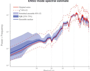
et al. (2011). In our case, the importance of this mode is mainly an artifact of dating errors. A spectral analysis of the age-perturbed PC (Fig. 5c, blue colors) shows a systematic increase in multidecadal variability (10–50-year periods) at the expense of interannual variability. The transfer of power from high to low frequencies may be seen by computing the spectral slopeβ, where we fit the model S(f )∝fβ to the continuum of each spectrum (f≤1/15). The spectrum of the unperturbed ENSO PC has a slope β◦= −0.72, while the age-perturbed ensemble shows values centered around a median valueβm= −0.22 with an interquartile range of [−0.41,0]. The loss of coherency thus has the effect of flat-tening the spectrum of the ENSO mode. Even when the error rate is 50 times smaller (θ=0.001), one still observes that age uncertainties tend to exaggerate multidecadal (20 years and longer) variations at the expense of interannual variations (Fig. 6). This may explain why Ault et al. (2009) found, using a similar PCA approach, that their coral network exhibited very energetic variability at such scales, with an amplitude that grew back in time. The presence of small age uncertain-ties could explain part of the multidecadal power enhance-ment they observed in the late nineteenth century, since fewer instrumental observations were available to provide chrono-logical anchors to coral time series at that time than in the twentieth century. Our analysis suggests that the accumula-tion of age model uncertainty is one possible – non-climatic – explanation for this apparent enhancement of low-frequency variability in an all-coral network, though a more detailed investigation (incorporating knowledge of error rates in each of their records) would be required to evaluate this quantita-tively.
4 Coherence-based identification of age models
As in Sect. 2.3, one would like to choose an optimal chronol-ogy among the ensemble of competing age models. To do so, we apply an optimization principle based on the idea that all pseudocorals in our network share some information about a common signal (ENSO in our pseudocoral benchmark). In-deed, coral networks have been shown to record spatiotem-porally coherent climate modes (Evans et al., 1998, 2000, 2002), a property shared by our pseudocoral network bench-mark (Fig. 5). Moreover, we showed in Sect. 3.3 that chrono-logical errors lead to a loss of coherency among records; that is, we expect age errors to lower interannual coherency among records compared to what it might otherwise be. While chronological uncertainty is not the only source of discrepancies among records (indeed the sampling of corals alone may be challenging due to their biologically mediated origins of layers), several studies (Hendy et al., 2002; De-Lon et al., 2007; DeDe-Long et al., 2013) highlight chronolog-ical uncertainties associated with coral reconstructions as a main cause for loss of coherency between records. One way to correct for this effect is to pick the age model that maxi-mizes interannual coherency between measurements.
50 20 10 5 2
10-6
10-5
10-4
10-3
Period (y)
Power
Frequency
ENSO mode spectral estimate
Original series
2 95% CI
Perturbed ensemble 95% CI IQR [25%-75%] Ensemble median
Fig. 6.Spectral density of the ENSO mode PC forθ=0.001. Com-pare to Fig. 5, bottom right.
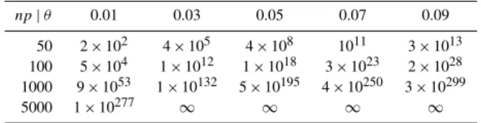
This exercise is, however, complicated by the large dimen-sionality of the space of possible solutions. The dimension-ality may be estimated in several ways: assuming that age perturbations follow a Bernoulli process, ann×pdata ma-trix admits up to 3npage perturbation matrices. This number quickly becomes astronomical, even for moderaten andp
(an NP-hard problem). A more relevant measure, however, is the number of solutions for a given error rate. Given a sym-metric error rateθ1=θ2=θ, one expects, on average, θ npgnp
(wherex˜denotes the nearest integer ofx) plausible solutions, which induces a serious computational challenge. This is il-lustrated in Table 2, which charts the number of solutions for various values ofnpandθ.
In practice, we generate an ensemble ofL=105time per-turbations1= {1(1), 1(2), . . . , 1(L)}according to Eq. (A5), and choose an optimal chronology amongst those realiza-tions. The optimization principle is described next.
4.1 Optimization scheme
Because age errors tend to lower coherency amongst records (Fig. 2), the quantity we seek to maximize is the generalized magnitude squared coherency (GMSC; Chakrabarty et al., 2002; Ramirez et al., 2008, 2010), an extension of the tra-ditional coherency to more than two time series. More pre-cisely, we maximize this quantity over the interannual band, where age perturbations have the largest effect on coherency. The method proceeds as described in Algorithm 1 (Table 3).
4.2 Method validation
Table 2.Complexity as a function ofθ and the matrix dimension
np. Infinity symbols denote numbers that exceed machine capacity.
np|θ 0.01 0.03 0.05 0.07 0.09
50 2×10² 4×10⁵ 4×10⁸ 1011 3×10¹³
100 5×10⁴ 1×10¹² 1×10¹⁸ 3×10²³ 2×1028
1000 9×1053 1×10132 5×10195 4×10250 3×10299
5000 1×10277 ∞ ∞ ∞ ∞
then generate an ensemble of age corrections (Sect. 3.1), for the reference perturbed data setC∗:= {ζ∗,τ∗}yielding an ensemble of candidate age-corrected data sets, and apply the optimization scheme described above. We then verify the va-lidity of our model by comparing the retained chronology to the true one.
For a given θ, the verification algorithm is explained in Algorithm 2 (Table 3).
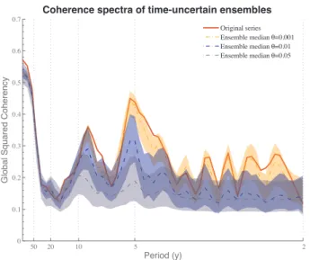
The results (Fig. 7) show the rapid loss of coherency over the interannual band as more age errors (increasingθ param-eter) are introduced in the time series. Indeed, theθ=0.001 case brings the vast majority of the time-uncertain ensemble spectra under the coherence spectrum of the original time series, and the θ=0.05 case suppresses nearly all the co-herency for periods shorter than 4 years, and greatly subdues the original peak around 5 years.
Forθ=0.05, the optimization principle failed to identify the correct age model, as no single realization of the cor-rected ensemble presented high GMSC values in the interan-nual band. The issue stems from the very high dimensionality of the space of plausible age corrections (Table 2), which re-sults in the inability of our sampled ensembles to span the solution space effectively. We attempted to use a Latin hy-percube sampling scheme in an effort to cover the solution space more effectively; however we did not notice any ma-jor improvement compared to the Monte Carlo ensemble re-sults. More work is required here to find efficient sampling techniques.
One way to evaluate the potential of this method to accu-rately portray uncertainties is to compute the actual coverage rates (Guttman, 1970) of CIs derived from our ensemble. To do so, we evaluate the probabilities that the ensemble CIs cover the original data set, and compare those to their nom-inal value of 95 % (Table 4). Asθincreases, so do time un-certainties, thereby widening the confidence interval of the ensemble. The coverage probability remains high for allθ, since the error-free data lie within the corrected ensemble nearly 98 % of the time. Our CIs are thus slightly conserva-tive.
While the difficulty in solving this NP-hard optimization problem gives little hope of finding the correct age model even for the smallestθ (note from Table 2 that the expected number of plausible chronologies to correct 1 % age errors is on the order of 1015), we here show that the coherence-based optimization principle can indeed bring the age model closer to the correct one.
To see this quantitatively, one first needs to define a distance over age model space. The Hamming distance
dH(x,y)(Hamming, 1950) between two vectorsxandyin Rn provides such a metric.dH(x,y)is defined as the pro-portion of corresponding coefficients positions in which they differ, i.e.,
dH(x,y)= 1
n
n
X
i=1
di,
where
di =
1 if xi=yi
0 otherwise. (3)
Because departures from unity in 1are of prime interest, this metric is a good one to differentiate time-shifted records from one another. We generalize the Hamming distance to our matrix case simply by computing and adding together the distances at each locationj, then dividing byp.
In the following experiment, we sample ensembles of chronologies in a restricted neighborhood around a reference age-perturbed data setC∗. In this context, for each time per-turbation inC∗, we sample an age correction within a neigh-borhood of size 2∗Nv+1, centered around a known mis-counted band.
Four age-corrected ensembles are generated using a neigh-borhood size expanding from Nv=1 to Nv=10 annual
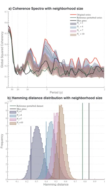
bands on either side of the true one. For each sampled re-alization, we evaluate the Hamming distance to the error-free chronology and compute the global coherence spectrum. For each ensemble, we construct its corresponding Hamming distance distribution and extract the realization that maxi-mizes the GMSC according to Algorithm 1 (Table 3). In Fig. 8, the results for each ensemble is color-coded so that one can relate the coherence spectra to the Hamming dis-tance distributions. The green color refers to the reference perturbed data set with an error rateθ=0.05, and the red is reserved for the original time series. The dark blue, blue, pink and light brown show the results forNv=1, 4, 7, and
10, respectively. We observe an increase in the mean of the distance distribution as the size of the neighborhoodNv
Table 3.Computational steps to identify an optimal chronology.
50 20 10 5 2
0 0.1 0.2 0.3 0.4 0.5 0.6 0.7
Period (y)
Global Squared Coherency
Coherence spectra of time-uncertain ensembles
Original series Ensemble median V=0.001 Ensemble median V=0.01 Ensemble median V=0.05
Fig. 7.Global coherence spectra for time-uncertain ensembles gen-erated withθ1=θ2=0.001 (orange),θ1=θ2=0.01 (dark blue) andθ1=θ2=0.05 (gray). The ensemble medians are illustrated in dashed lines, and their corresponding colored patches represent the ensemble 95 % CIs. The thick red curve is the coherence spectrum of the error-free time series.
Table 4.Time-uncertain ensemble 95 % CI width meansµand stan-dard deviationsσ, and probabilities of the ensemble CI covering the original data with respect toθ.
θ 0.01 0.03 0.05 0.07 0.09
CI width,µ 0.38 0.47 0.50 0.53 0.55
CI width,σ 0.18 0.17 0.17 0.16 0.17
Coverage rate 0.97 0.99 0.97 0.98 0.98
the realization that achieves the maximum GMSC value, se-lected from an unrestricted ensemble such as one generated according to Eq. (A5). The sampling issue associated with the extremely high dimensionality of the solution space can be readily observed here, noticing that the realization maxi-mizing the GMSC barely surpasses the reference coherence spectrum in addition to its distance to the original chronology exceeding the distance between the reference and true data. The issue may be alleviated if there is some prior informa-tion about the timing of age errors, for instance an observed mismatch between how two series portray an event – like a historic volcanic eruption – that should be synchronous.
5 Discussion
In this article, we put forth a probabilistic model for layer-counted chronologies. The model was designed for univariate as well as multivariate data sets, and is flexible enough to ac-commodate location-specific and asymmetric error rates. We used this model to generate ensembles of time-uncertain data sets, which we analyzed using spectral methods and principal component analysis.
In the univariate case, we showed that age perturba-tions tend to blur variability between interannual and multi-decadal scales. In the multivariate case, we showed that even small age offsets between records may significantly lower coherency between records, producing an apparent ampli-tude modulation of high-frequency signals. These short-term phase interferences thus led to long-term effects, exaggerat-ing low-frequency variability at the expense of interannual signals. This suggests that at least part of the reason for the observed nineteenth century increase in the amplitude of low-frequency variability (Ault et al., 2009) could be the presence of age errors.
50 20 10 5 2 0
0.1 0.2 0.3 0.4 0.5 0.6 0.7
Period (y)
Global Squared Coherency
a) Coherence Spectra with neighborhood size
Original series Reference perturbed series Max gmsc Nv = 1 N
v = 4
N
v = 7
N
v = 10
0 0.1 0.2 0.3 0.4 0.5 0.6 0.7 0.8 0.9 1
0 1 2 3 4 5 6 7 8 9 10x 10
4
Hamming distance
Frequency
b) Hamming distance distribution with neighborhood size
Reference perturbed dataset Max gmsc
N v=1 N
v=4 Nv=7 Nv=10
Fig. 8.Coherence spectra (top) and Hamming distance distributions to the original chronology (bottom) for ensembles of chronologies sampled around the reference perturbation matrix (withθ=0.05), in restricted neighborhood of sizes 2∗Nv+1 for Nv increasing from 1 to 10. The thick red curve represents the coherence spec-trum for the error-free data, the results related to the reference per-turbed data set are shown in green, and plotted in black are the re-sults for the ensemble realization (sampled across the entire solution space) that maximizes the GMSC for the neighborhood ensembles (shaded areas): the 95 % CIs and Hamming distance distributions, and corresponding realizations maximizing the GMSC (solid lines) are shown in dark blue, blue, pink and light brown forNv=1, 4, 7 and 10, respectively.
There are important limitations to our study. First and fore-most, our framework assumes that the error rates are known. Ideally, one would estimate the miscounting rate parameters
(θ1, θ2)from the data, which could be done in the presence of
independent information (replicated annual cycles in multi-ple types of observations, absolute or independent age infor-mation), and/or information such as the cumulative number
of material hiatuses, which may be correlated to the likeli-hood of missing or double-counted events (e.g., Brown et al., 1992; Alley et al., 1997a; Juillet-Leclerc et al., 2006; Alibert and Kinsley, 2008; DeLong et al., 2013). Future work with the uncertainty algorithm might use such information to em-pirically and adaptively reset accumulated age errors.
We also restricted our analysis to symmetric error rates, which is an unlikely scenario according to DeLong et al. (2013), who emphasized that double counting is typically more common than missing years in coral records from the reefs offshore of Amédée Island. Considering that the events perturbing the chronologies are hidden states of the pro-cess and are not being directly measured, a maximum likeli-hood principle would have to be employed to evaluate the error rate, which substantially complicates the problem of designing a likelihood function. However, when the com-mon signal driving the record is strong enough, a coherency-based Bayesian approach could potentially learn from the data. In this case, one would relax the assumption of known miscounting rate parameters (θ1, θ2)in favor of prior
dis-tributions on those parameters, which would incorporate as much scientific information as possible. In this regard, one should note that most geochronologies are developed with the purpose of producing the single best representation of past changes. There would be merit in also providing raw chronologies so that the error rate may be estimated via com-paring it with other, absolutely dated records (for instance, historical observations or chronostratigraphic markers). In other words, we urge field scientists to report all the chrono-logical information relevant to the characterization of these error rates, rather than exclusively seeking to reduce them, as this would greatly aid the quantification of uncertainties associated with each record.
Second, we assumed that time perturbations follow a ho-mogeneous Poisson process, with a uniform and symmetric rate for all pseudocorals considered. In nature, each record will display a different rate, and in situations of uneven dat-ing conditions (e.g., annual bands bedat-ing more or less visible in a given time interval; see Fig. 1b) an inhomogeneous Pois-son process would constitute a more suitable model within a single record. The error rate could change with the location and age of the sample, and be informed by local expertise to account for known climatic events that could have affected the coral growth structures. Assessments of where and when corals might have over- or undergrown impose restrictions on the age model space, which would greatly improve the ability of our optimization principle to identify the correct chronology.
perturbations, which could be done by specifying parameters conditional on the climate.
Fourth, we assumed that all records considered had annual resolution, while in reality it could range from a month to several years. Adapting the method to a network of variable resolution would require the conditioning of the error rate parameterθon the resolution of the record’s chronology. For instance, monthly data tend to present a lower error rate than yearly data, due the presence of a well-defined annual cy-cle, i.e., a seasonal cycle inδ18O in one or more paleodata streams from the coral (and other annually layered archives) that mostly “resets” age model uncertainty at some point in the year. Yet monthly data would add subannual errors from selecting incorrect tie points in the seasonal cycle and from interpolating between tie points (e.g., De Ridder et al., 2004), particularly in regions where the seasonal cycle and annual density banding are weak (e.g., key ENSO-sensitive regions of the central Pacific, Fig. 1b). Likewise, multiple-year sam-pling intervals could have aliasing consequences that would potentially add to age uncertainties.
Fifth, we assumed that the latest timetfis known exactly
(except in Sect. 2.3), which is only true of records that grew continuously until that point (e.g., living corals, living trees). We could refine our fossil corals framework with a mixed approach, where the age of tie points would be allowed to vary according to their distribution (e.g., a Gaussian), and the layer-count model would be extended on either side.
Finally, our optimization scheme was shown to be effec-tive only in extremely restricted situations (error-free mea-surements ofδ18O, age model ensemble spanning the true-age model). It remains to be seen whether these conditions could ever be met in practice. One potential problem is the fact that the “clock” used to synchronize the records does not beat periodically: ENSO is only a quasi-periodic phe-nomenon, even in the GFDL CM2.0 model. Perhaps a more regular (annual, semi-annual) cycle would provide stronger synchronization constraints (but it would limit the analysis to records that have seasonal or better resolution). Alterna-tively, one could restrict the optimization process to small, regional ensembles of proxies that share a stronger common signal, much like dendrochronological approaches.
With these caveats in mind, several points deserve men-tion. First, the simple example of Fig. 2 demonstrates how miscounting errors may produce an apparent amplitude mod-ulation of otherwise stationary signals, producing spurious trends in the average derived from them. Because climate re-construction methods rely in some fashion on a weighted av-erage of observations assumed to be contemporaneous, this may partially explain why many ENSO reconstructions (e.g., Mann et al., 2000; Wilson et al., 2010; McGregor et al., 2010; Li et al., 2011; Emile-Geay et al., 2013) display increasing trends in ENSO variance over time (McGregor et al., 2013). As pointed out in the latter study, computing ENSO vari-ance on individual records prior to averaging them together is more robust to chronological errors. In the meantime,
inter-preting trends in variance obtained from the average of age-uncertain records as reflecting a response to external forc-ing may be perilous. At the very least, a probabilistic model such as the one proposed here can provide a null hypothesis against which to assess such trends.
More generally, a model such as this one may be used to evaluate the plausible impact of dating uncertainties on all manner of inferences derived from time-uncertain records. Just as proxy system models are now becoming a standard tool to interpret environmental controls in paleoclimate prox-ies, chronological models should become an integral com-ponent of proxy system models for age-uncertain paleodata, so that they may be used to improve interpretation, recon-struction, uncertainty estimation, and data–model compari-son studies (Evans et al., 2013). Because chronological errors might themselves depend on climatic events (see Introduc-tion), a complete proxy system model should in fact allow environmental controls to influence chronological informa-tion.
We hope this study stimulates a discussion on how to best represent chronological uncertainty in layer-counted proxy archives and leads to a better characterization of these uncer-tainties.
Acknowledgements. M. Comboul, J. Emile-Geay, M. N. Evans,
N. Mirnateghi, and D. M. Thompson acknowledge funding from NOAA award NA10OAR4310115. The authors also acknowledge the anonymous reviewer’s effort in making useful comments that improved the paper. Matlab code implementing the age model ensembles is freely available on the Common Climate Google Code repository (https://code.google.com/p/common-climate/) (will be released after manuscript acceptance).
Edited by: P. Braconnot
References
Abram, N. J., Gagan, M. K., Cole, J. E., Hantoro, W. S., and Mudelsee, M.: Recent intensification of tropical climate variability in the Indian Ocean, Nat. Geosci., 1, 849–853, doi:10.1038/ngeo357, 2008.
Abramowitz, M. and Stegun, I. A.: Handbook of Mathematical Functions, National Bureau of Standards, Applied Math # 55, Dover Publications, 1965.
Alibert, C. and Kinsley, L.: A 170-year Sr/Ca and Ba/Ca coral record from the western Pacific warm pool: 2. A window into variability of the New Ireland Coastal Undercurrent, J. Geophys. Res., 113, 1–10, doi:10.1029/2007JC004263, 2008.
Alley, R. B., Mayewski, P. A., Sowers, T., Stuiver, M., Taylor, K. C., and Clark, P. U.: Holocene climatic instability: A promi-nent, widespread event 8200 yr ago, Geology, 25, 483–486, doi:10.1130/0091-7613(1997)025<0483:HCIAPW>2.3.CO;2, 1997a.
of the GISP2 ice core: Basis, reproducibility, and application, J. Geophys. Res., 102, 26367–26381, doi:10.1029/96JC03837, 1997b.
Anchukaitis, K. J. and Tierney, J. E.: Identifying coherent spa-tiotemporal modes in time-uncertain proxy paleoclimate records, Clim. Dynam., 41, 1291–1306, doi:10.1007/s00382-012-1483-0, 2012.
Asami, R., Yamada, T., Iryu, Y., Quinn, T. M., Meyer, C. P., and Pauley, G.: Interannual and decadal variability of the western Pa-cific sea surface condition for the years 1787-2000: Reconstruc-tion based on stable isotope record from a Guam coral, J. Geo-phys. Res., 110, C05018, doi:10.1029/2004JC002555, 2005. Ault, T. R., Cole, J. E., Evans, M. N., Barnett, H., Abram, N. J.,
Tudhope, A. W., and Linsley, B. K.: Intensified decadal variabil-ity in tropical climate during the late 19th century, Geophys. Res. Lett., 36, L08602, doi:10.1029/2008GL036924, 2009.
Bender, M. L.: Orbital tuning chronology for the Vostok climate record supported by trapped gas composition, Earth Planet. Sc. Lett., 204, 275–289, doi:10.1016/S0012-821X(02)00980-9, 2002.
Blaauw, M.: Methods and code for “classical” age-modelling of radiocarbon sequences, Quat. Geochronol., 5, 512 – 518, doi:10.1016/j.quageo.2010.01.002, 2010.
Blaauw, M.: Out of tune: the dangers of aligning
proxy archives, Quaternary Sci. Rev., 36, 38–49,
doi:10.1016/j.quascirev.2010.11.012, 2012.
Blaauw, M. and Christen, J. A.: Flexible paleoclimate age-depth models using an autoregressive gamma process, Bayesian Anal-ysis, 6, 457–474, doi:10.1214/11-BA618, 2011.
Boiseau, M., Juillet-Leclerc, A., Yiou, P., Salvat, B., Isdale, P., and Guillaume, M.: Atmospheric and oceanic evidences of El Niño-Southern Oscillation events in the south central Pacific Ocean from coral stable isotopic records over the last 137 years, Paleo-ceanography, 13, 671–685, doi:10.1029/98PA02502, 1998. Breitenbach, S. F. M., Rehfeld, K., Goswami, B., Baldini, J. U. L.,
Ridley, H. E., Kennett, D. J., Prufer, K. M., Aquino, V. V., As-merom, Y., Polyak, V. J., Cheng, H., Kurths, J., and Marwan, N.: COnstructing Proxy Records from Age models (COPRA), Clim. Past, 8, 1765–1779, doi:10.5194/cp-8-1765-2012, 2012. Broomhead, D. and King, G. P.: Extracting qualitative
dy-namics from experimental data, Physica D, 20, 217–236, doi:10.1016/0167-2789(86)90031-X, 1986.
Brown, F. H., Sarna-Wojcicki, A. M., Meyer, C. E., and Haileab, B.: Correlation of Pliocene and Pleistocene tephra layers between the Turkana Basin of East Africa and the Gulf of Aden, Quatern. Int., 13–14, 55–67, doi:10.1016/1040-6182(92)90010-Y, 1992. Calvo, E., Marshall, J. F., Pelejero, C., McCulloch, M. T., Lough,
J. M., and Isdale, P. J.: Interdecadal climate variability in the Coral Sea since 1708 A.D., Palaeogeogr. Palaeocl„ 248, 190– 201, 2007.
Capotondi, A., Wittenberg, A., and Masina, S.: Spatial and temporal structure of tropical Pacific interannual variability in 20th century coupled simulations, Ocean Model., 15, 274–298, 2006. Chakrabarty, K., Sitharama Iyengar, S., Qi, H., and Cho, E.: Grid
Coverage for Surveillance and Target Location in Distributed Sensor Networks, IEEE T. Comput., 51, 1448–1453, 2002. Charles, C. D., Hunter, D. E., and Fairbanks, R. G.:
Inter-action Between the ENSO and the Asian Monsoon in a
Coral Record of Tropical Climate, Science, 277, 925–928, doi:10.1126/science.277.5328.925, 1997.
Charles, C. D., Cobb, K., Moore, M. D., and Fairbanks, R. G.: Monsoon-tropical ocean interaction in a network of coral records spanning the 20th century, Mar. Geol., 201, 207–222, doi:10.1016/S0025-3227(03)00217-2, 2003.
Chave, A. D., Thomson, D. J., and Ander, M. E.: On the robust estimation of power spectra, coherences, and transfer functions, J. Geophys. Res., 92, 633–648, doi:10.1029/JB092iB01p00633, 1987.
Cobb, K. M., Charles, C. D., and Hunter, D. E.: A central trop-ical Pacific coral demonstrates Pacific, Indian, and Atlantic decadal climate connections, Geophys. Res. Lett., 28, 2209– 2212, doi:10.1029/2001GL012919, 2001.
Cobb, K. M., Charles, C. D., Cheng, H., and Edwards, R. L.: El Niño/Southern Oscillation and tropical Pacific climate during the last millennium, Nature, 424, 271–276, 2003.
Cobb, K. M., Westphal, N., Sayani, H. R., Watson, J. T., Lorenzo, E. D., Cheng, H., Edwards, R. L., and Charles, C. D.: Highly Variable El Niño-Southern Oscillation Throughout the Holocene, Science, 339, 67–70, 2013.
Cook, E. R. and Kairiukstis, L. A.: Methods of dendrochronology: Applications in the environmental sciences, Springer, ISBN: 0-7923-0586-8, 1990.
Damassa, T. D., Cole, J. E., Barnett, H. R., Ault, T. R., and McClanahan, T. R.: Enhanced multidecadal climate variabil-ity in the seventeenth century from coral isotope records in the western Indian Ocean, Paleoceanography, 21, PA2016, doi:10.1029/2005PA001217, 2006.
De Ridder, F., Pintelon, R., Schoukens, J., Gillikin, D. P., André, L., Baeyens, W., de Brauwere, A., and Dehairs, F.: Decoding nonlin-ear growth rates in biogenic environmental archives, Geochem. Geophy. Geosy., 5, doi:10.1029/2004GC000771, 2004. DeLong, K. L., Quinn, T. M., and Taylor, F. W.:
Reconstruct-ing twentieth-century sea surface temperature variability in the southwest Pacific: A replication study using multiple coral Sr/Ca records from New Caledonia, Paleoceanography, 22, PA4212, doi:10.1029/2007PA001444, 2007.
DeLong, K. L., Flannery, J. A., Maupin, C. R., Poore, R. Z., and Quinn, T. M.: A coral Sr/Ca calibration and replication study of two massive corals from the Gulf of Mexico, Palaeogeogr. Palaeocl., 307, 117–128, 2011.
DeLong, K. L., Quinn, T. M., Taylor, F. W., Shen, C.-C., and Lin, K.: Improving coral-base paleoclimate reconstructions by replicating 350 years of coral Sr/Ca variations, Palaeogeogr. Palaeocl., 373, 6–24, 2013.
Douglass, A. E.: Crossdating in dendrochronology, J. Forest., 39, 825–831, 1941.
Emile-Geay, J. and Eshleman, J. A.: Toward a semantic web of paleoclimatology, Geochem. Geophy. Geosy., 14, 457–469, doi:10.1002/ggge.20067, 2013.
Emile-Geay, J., Cobb, K., Mann, M., and Wittenberg, A. T.: Esti-mating Central Equatorial Pacific SST variability over the Past Millennium. Part 2: Reconstructions and Implications, J. Cli-mate, 26, 2329–2352, doi:10.1175/JCLI-D-11-00511.1, 2013. Evans, M., Tolwinski-Ward, S., Thompson, D., and Anchukaitis,
Evans, M. N., Kaplan, A., and Cane, M. A.: Optimal sites for coral-based reconstruction of global sea surface temperature, Paleo-ceanography, 13, 502–516, doi:10.1029/98PA02132, 1998. Evans, M. N., Kaplan, A., and Cane, M. A.: Intercomparison of
coral oxygen isotope data and historical sea surface temperature (SST): Potential for coral-based SST field reconstructions, Pale-oceanogr., 15, 551–562, 2000.
Evans, M. N., Kaplan, A., and Cane, M. A.: Pacific sea sur-face temperature field reconstruction from coralδ18O data us-ing reduced space objective analysis, Paleoceanogr., 17, 7–1, doi:10.1029/2000PA000590, 2002.
Fairbanks, R. G. and Dodge, R. E.: Annual periodicity of the 18O/16O and13C/12C ratios in the coralMontastrea annularis,
Geochim. Cosmochim. Ac., 43, 1009–1020, 1979.
Felis, T., Pätzold, J., Loya, Y., Fine, M., Nawar, A. H., and Wefer, G.: A coral oxygen isotope record from the northern Red Sea documenting NAO, ENSO, and North Pacific teleconnections on Middle East climate variability since the year 1750, Paleo-ceanography, 15, 679–694, doi:10.1029/1999PA000477, 2000. Fraedrich, K.: Estimating the Dimensions of Weather and
Cli-mate Attractors, J.Atmos. Sci., 43, 419–432, doi:10.1175/1520-0469(1986)043<0419:ETDOWA>2.0.CO;2, 1986.
Fritts, H. C.: Tree Rings and Climate, 567 pp., Academic Press, 1976.
Grootes, P. M., Stuiver, M., White, J. W. C., Johnsen, S., and Jouzel, J.: Comparison of oxygen isotope records from the GISP2 and GRIP Greenland ice cores, Nature, 366, 552–554, doi:10.1038/366552a0, 1993.
Guttman, I.: Statistical tolerance regions: classical and Bayesian, vol. 26, Griffin London, 1970.
Haam, E. and Huybers, P.: A test for the presence of covariance between time-uncertain series of data with application to the Dongge Cave speleothem and atmospheric radiocarbon records, Paleoceanography, 25, PA2209, doi:10.1029/2008PA001713, 2010.
Hamming, R. W.: Error Detecting and Error Correcting Codes, Bell Syst. Tech. J., 29, 147–160, 1950.
Hays, J. D., Imbrie, J., and Shackleton, N. J.: Variations in the Earth’s Orbit: Pacemaker of the Ice Ages, Science, 194, 1121– 1132, 1976.
Hendy, E. J., Gagan, M. K., Alibert, C. A., McCulloch, M. T., Lough, J. M., and Isdale, P. J.: Abrupt Decrease in Tropical Pa-cific Sea Surface Salinity at End of Little Ice Age, Science, 295, 1511–1514, doi:10.1126/science.1067693, 2002.
Huybers, P. and Wunsch, C.: A depth-derived Pleistocene age model: Uncertainty estimates, sedimentation variability, and nonlinear climate change, Paleoceanogr., 19, PA1028, doi:10.1029/2002PA000857, 2004.
Isdale, P. J., Stewart, B. J., Tickle, K. S., and Lough, J. M.: Palaeohydrological variation in a tropical river catch-ment: a reconstruction using fluorescent bands in corals of the Great Barrier Reef, Australia, The Holocene, 8, 1–8, doi:10.1191/095968398670905088, 1998.
Juillet-Leclerc, A., Thiria, S., Naveau, P., Delcroix, T., Le Bec, N., Blamart, D., and Corrège, T.: SPCZ migration and ENSO events during the 20th century as revealed by climate prox-ies from a Fiji coral, Geophys, Res. Lett., 33, L17710, doi:10.1029/2006GL025950, 2006.
Knutson, T. R., Delworth, T. L., Dixon, K. W., Held, I. M., Lu, J., Ramaswamy, V., Schwarzkopf, M. D., Stenchikov, G., and Stouf-fer, R. J.: Assessment of Twentieth-Century Regional Surface Temperature Trends Using the GFDL CM2 Coupled Models, J. Climate, 19, 1624–1651, doi:10.1175/JCLI3709.1, 2006. Kug, J.-S., Choi, J., An, S.-I., Jin, F.-F., and Wittenberg, A. T.:
Warm pool and cold tongue El Niño events as simulated by the GFDL CM2.1 coupled GCM, J. Climate, 23, 1226–1239, doi:10.1175/2009JCLI43293.1, 2010.
Kuhnert, H., Pätzold, J., Hatcher, B., Wyrwoll, K. H., Eisen-hauer, A., Collins, L. B., Zhu, Z. R., and Wefer, G.: A 200-year coral stable oxygen isotope record from a high-latitude reef off Western Australia, Coral Reefs, 18, 1–12, doi:10.1007/s003380050147, 1999.
Kuhnert, H., Pätzold, J., Wyrwoll, K.-H., and Wefer, G.: Monitoring climate variability over the past 116 years in coral oxygen iso-topes from Ningaloo Reef, Western Australia, Int. J. Earth Sci., 88, 725–732, doi:10.1007/s005310050300, 2000.
Li, J., Xie, S.-P., Cook, E. R., Huang, G., D’Arrigo, R., Liu, F., Ma, J., and Zheng, X.-T.: Interdecadal modulation of El Niño amplitude during the past millennium, Nature Climate Change, 1, 114–118, 2011.
Linsley, B. K., Dunbar, R. B., Wellington, G. M., and Mucciarone, D. A.: A coral-based reconstruction of intertropical convergence zone variability over Central America since 1707, J. Geophys. Res., 99, 9977–9994, doi:10.1029/94JC00360, 1994.
Linsley, B. K., Ren, L., Dunbar, R. B., and Howe, S. S.: El Niño Southern Oscillation (ENSO) and decadal-scale climate variabil-ity at 10◦N in the eastern Pacific from 1893 to 1994: A coral-based reconstruction from Clipperton Atoll, Paleoceanography, 15, 322–335, doi:10.1029/1999PA000428, 2000.
Linsley, B. K., Kaplan, A., Gouriou, Y., Salinger, J., deMenocal, P. B., Wellington, G. M., and Howe, S. S.: Tracking the extent of the South Pacific Convergence Zone since the early 1600s, Geochem. Geophy. Geosy., 7, doi:10.1029/2005GC001115, 2006.
Linsley, B. K., Zhang, P., Kaplan, A., Howe, S. S., and Welling-ton, G. M.: Interdecadal-decadal climate variability from multi-coral oxygen isotope records in the South Pacific Convergence Zone region since 1650 A.D., Paleoceanography, 23, PA2219, doi:10.1029/2007PA001539, 2008.
Lisiecki, L. E. and Raymo, M. E.: A Pliocene-Pleistocene stack of 57 globally distributed benthicδ18O records, Paleoceanography, 20, PA1003, doi:10.1029/2004PA001071, 2005.
Mann, M., Gilleb, E., Bradley, R., Hughes, M., Overpeck, J., Keimigc, F., and Gross, W.: Global temperature patterns in past centuries: An interactive presentation, Earth Interact., 4, 1–29, 2000.
Marcott, S. A., Shakun, J. D., Clark, P. U., and Mix, A. C.: A Recon-struction of Regional and Global Temperature for the Past 11,300 Years, Science, 339, 1198–1201, doi:10.1126/science.1228026, 2013.
Martinson, D. G., Menke, W., and Stoffa, P.: An Inverse Ap-proach to Signal Correlation, J. Geophys. Res., 87, 4807–4818, doi:10.1029/JB087iB06p04807, 1982.
McGregor, S., Timmermann, A., England, M. H., Elison Timm, O., and Wittenberg, A. T.: Inferred changes in El Niño-Southern Os-cillation variance over the past six centuries, Clim. Past, 9, 2269– 2284, doi:10.5194/cp-9-2269-2013, 2013.
Mudelsee, M., Scholz, D., Röthlisberger, R., Fleitmann, D., Mangini, A., and Wolff, E. W.: Climate spectrum estimation in the presence of timescale errors, Nonlin. Processes Geophys., 16, 43–56, doi:10.5194/npg-16-43-2009, 2009.
PAGES2K Consortium: Continental-scale temperature variabil-ity during the past two millennia, Nat. Geosci, 6, 339–346, doi:10.1038/ngeo1797, 2013.
Pfeiffer, M., Timm, O., Dullo, W.-C., and Podlech, S.: Oceanic forcing of interannual and multidecadal climate variability in the southwestern Indian Ocean: Evidence from a 160 year coral iso-topic record (La Réunion, 55◦E, 21◦S), Paleoceanography, 19, doi:10.1029/2003PA000964, 2004.
Quinn, T. M., Crowley, T. J., Taylor, F. W., Henin, C., Joannot, P., and Join, Y.: A multicentury stable isotope record from a New Caledonia coral: Interannual and decadal sea surface tempera-ture variability in the southwest Pacific since 1657 A.D., Paleo-ceanography, 13, 412–426, doi:10.1029/98PA00401, 1998. Quinn, T. M., Taylor, F. W., and Crowley, T. J.: Coral-based climate
variability in the Western Pacific Warm Pool since 1867, J. Geo-phys. Res., 111, C11006, doi:10.1029/2005JC003243, 2006. Ramirez, D., Via, J., and Santamaria, I.: A generalization of the
magnitude squared coherence spectrum for more than two sig-nals: definition, properties and estimation, in: Acoustics, Speech and Signal Processing, 2008. ICASSP 2008. IEEE Interna-tional Conference on, 31 March–4 April 2008, 3769–3772, doi:10.1109/ICASSP.2008.4518473, 2008.
Ramirez, D., Via, J., Santamaria, I., and Scharf, L. L.: Detection of Spatially Correlated Gaussian Time Series, IEEE T. Signal Pro-ces., 58, 5006–5015, 2010.
Rhines, A. and Huybers, P.: Estimation of spectral power laws in time uncertain series of data with application to the Greenland Ice Sheet Project 2δ18O record, J. Geophys. Res., 116, D01103, doi:10.1029/2010JD014764, 2011.
Schoellhamer, D. H.: Singular spectrum analysis for time se-ries with missing data, Geophys. Res. Lett., 28, 3187–3190, doi:10.1029/2000GL012698, 2001.
Seimon, A.: Improving climatic signal representation in tropical ice cores: A case study from the Quelccaya Ice Cap, Peru, Geophys. Res. Lett., 30, 1772, doi:10.1029/2003GL017191, 2003. Shen, C.-C., Lin, K., Duan, W., Jiang, X., Partin, J. W.,
Ed-wards, R. L., Cheng, H., and Tan, M.: Testing the annual nature of speleothem banding, Scientific Reports, 3, 2633, doi:10.1038/srep02633, 2013.
Skellam, J. G.: The Frequency Distribution of the Difference Be-tween Two Poisson Variates Belonging to Different Populations, J. R. Stat. Soc. Ser. A-G., 109, 296 pp., 1946.
St. George, S., Ault, T. R., and Torbenson, M. C. A.: The rarity of absent growth rings in Northern Hemisphere forests outside the American Southwest, Geophys. Res. Lett., 40, 3727–3731, doi:10.1002/grl.50743, 2013.
Stokes, M. A. and Smiley, T. L.: An Introduction to Tree-Ring Dat-ing, The University of Chicago Press, 1996.
Suhov, Y. and Kelbert, M.: Probability and statistics by example: Markov chains: a primer in random processes and their applica-tions, Cambridge University Press, 2008.
Thompson, D. M., Ault, T. R., Evans, M. N., Cole, J. E., and Emile-Geay, J.: Comparison of observed and simulated tropical climate
trends using a forward model of coral ofδ18O, Geophys. Res.
Lett., 38, L14706, doi:10.1029/2011GL048224, 2011.
Thompson, L. G., Mosley-Thompson, E., Bolzan, J. F., and Koci, B. R.: A 1500-Year Record of Tropical Precipitation in Ice Cores from the Quelccaya Ice Cap, Peru, Science, 229, 971–973, doi:10.1126/science.229.4717.971, 1985.
Thomson, D. J.: Spectrum estimation and harmonic analysis, Pro-ceedings of the IEEE, 70, 1055–1096, 1982.
Tierney, J. E., Smerdon, J. E., Anchukaitis, K. J., and Sea-ger, R.: Multidecadal variability in East African hydrocli-mate controlled by the Indian Ocean, Nature, 493, 389– 392,doi:10.1038/nature11785, 2013.
Tingley, M. P. and Huybers, P.: Recent temperature extremes at high northern latitudes unprecedented in the past 600 years, Nature, 496, 201–205, doi:10.1038/nature11969, 2013.
Tudhope, A. W., Chilcott, C. P., McCulloch, M. T., Cook, E. R., Chappell, J., Ellam, R. M., Lea, D. W., Lough, J. M., and Shim-mield, G. B.: Variability in the El Niño-Southern Oscillation Through a Glacial-Interglacial Cycle, Science, 291, 1511–1517, doi:10.1126/science.1057969, 2001.
Urban, F. E., Cole, J. E., and Overpeck, J. T.: Influence of mean climate change on climate variability from a 155-year tropical Pacific coral record, Nature, 407, 989–993, 2000.
Vautard, R. and Ghil, M.: Singular spectrum analysis in nonlinear dynamics, with applications to paleoclimatic time series, Phys-ica D, 35, 395–424, 1989.
Vecchi, G. A., Soden, B. J., Wittenberg, A. T., Held, I. M., Leet-maa, A., and Harrison, M. J.: Weakening of tropical Pacific at-mospheric circulation due to anthropogenic forcing, Nature, 441, 73–76, 2006.
Wang, Y. J., Cheng, H., Edwards, R. L., An, Z. S., Wu, J. Y., Shen, C.-C., and Dorale, J. A.: A High-Resolution Absolute-Dated Late Pleistocene Monsoon Record from Hulu Cave, China, Science, 294, 2345–2348, doi:10.1126/science.1064618, 2001.
Wigley, T. M. L., Jones, P. D., and Briffa, K. R.: Cross-dating meth-ods in dendrochronology, J. Archaeol. Sci., 14, 51–64, 1987. Wilson, R., Cook, E., D’Arrigo, R., Riedwyl, N., Evans, M. N.,
Tudhope, A., and Allan, R.: Reconstructing ENSO: the influence of method, proxy data, climate forcing and teleconnections, J. Quaternary Sci., 25, 62–78, doi:10.1002/jqs.1297, 2010. Wittenberg, A. T., Rosati, A., Lau, N.-C., and Ploshay, J. J.:
GFDL’s CM2 Global Coupled Climate Models. Part III: Trop-ical Pacific Climate and ENSO, J. Climate, 19, 698–722, doi:10.1175/JCLI3631.1, 2006.
Xie, S.-P., Deser, C., Vecchi, G. A., Ma, J., Teng, H., and Wittenberg, A. T.: Global warming pattern formation: Sea surface temperature and rainfall, J. Climate, 23, 966–986, doi:10.1175/2009JCLI3329.1, 2010.
Yamaguchi, D. K.: A simple method for cross-dating increment cores from living trees, Can. J. Forest Res., 21, 414–416, 1991. Zinke, J., Dullo, W.-C., Heiss, G. A., and Eisenhauer, A.: ENSO