Wind-induced baroclinic response of Lake Constance

Wind-induced baroclinic response of Lake Constance

Y. Wang1, K. Hutter1, E. BaÈuerle2 1

Institute of Mechanics, Darmstadt University of Technology, Hochschulstr. 1, D-64289 Darmstadt, Germany

2_{Limnological Institute, University of Constance, D-78457 Constance, Germany}

Received: 23 February 2000 / Revised: 14 June 2000 / Accepted: 5 July 2000

Abstract. We present results of various circulation scenarios for the wind-induced three-dimensional cur-rents in Lake Constance, obtained with the aid of a semi-spectral semi-implicit ®nite di€erence code devel-oped in Haidvogelet al. and Wang and Hutter. Internal Kelvin and PoincareÂ-type oscillations are demonstrated in the numerical results, whose periods depend upon the strati®cation and the geometry of the basin and agree well with measured data. By solving the eigenvalue problem of the linearized shallow water equations in the two-layered strati®ed Lake Constance, the interpreta-tion of the oscillainterpreta-tions as Kelvin and PoincareÂ-type waves is corroborated.

Key words: Oceanography: general (limnology;

numerical modeling) ± Oceanography: physical (internal and inertial waves)

1 Introduction

The strati®cation in lakes is almost exclusively estab-lished by the heat input due to solar radiation. During the summer season, in temperate climate zones, a strati®cation given at one particular instant generally persists for a time span that is long in comparison to the time scales of the dynamic circulation which is estab-lished by the wind shear traction applied at the water surface. Only during short-lived episodes, when the shearing in the surface layer is very large (i.e., typically during strong storms), Kelvin-Helmholtz instabilities can form which then generate internal bores that destroy the strati®cation or may erode the thermocline. During the periods in between the change in mass distribution due to circulation dynamics is relatively small. Thus, a

stable underlying strati®cation with no movement may be assumed as an initial condition from which the temperature and velocity ®eld may develop without forming internal instabilities.

The underlying thermo-mechanical processes can be described mathematically by the shallow water equations in the Boussinesq approximation: in these equations the vertical momentum balance reduces to the force balance between pressure gradient and gravity (buoyancy) force, and density variations are only accounted for in the buoyancy term. The equations describe both, barotropic and baroclinic processes. The former are those that develop when density variations do not exist and, in temperate zones, arise in late autumn and during winter. They also exist in a truly strati®ed lake or ocean basin, but are then overshadowed by the baroclinic processes that are typical for the summer seasons when the underlying strati®cation is strong.

There are many numerical models based on the shallow water equations in the Boussinesq approxima-tion (Ramming and Kowalik, 1980; Simons, 1980; Oman, 1982; Pohlmann, 1987; Tee, 1987; Lehmann, 1995). Haidvogel and Beckmann (1998) also summa-rized many such three-dimensional models. All claim to describe these kind of wind-induced motions, and have been applied to large-scale oceanographic situations. Some three-dimensional models have been used to describe circulation ¯ows in lakes and have had limited success (e.g. Bennett, 1977; Hollan and Simons, 1978; Oman, 1982). However these three-dimensional models or codes are limited in their applicability, or unsatisfac-tory, because internal wave processes are overly damped owing to the large explicit or implicit numerical di€u-sion that had to be built into the codes to stabilize them under common conditions.

Here, the nonlinear shallow water equations in the Boussinesq approximation, that describe wind induced circulation dynamics in enclosed basins, are integrated using a numerical semi-spectral primitive equation model (SPEM) that was modi®ed by us with a semi-implicit time-integration in the vertical direction. For greater detail the reader is referred to Wang and Hutter Correspondence to: Y. Wang

(1998). Here our aim is the presentation of solutions to a given initial strati®cation and a wind stress from di€erent directions.

In Sect. 2 we brie¯y outline the model. In Sect. 3 various scenarios of wind-driven baroclinic processes in Lake Constance are studied and the predicted Kelvin and PoincareÂ-type oscillations can be displayed in the results. In Sect. 4, by solving the eigenvalue problem of the linearized shallow water equations of the two-layered Lake Constance, the interpretation of the oscillations as Kelvin and PoincareÂ-type waves can be ascertained. We conclude with a summary and some remarks in Sect. 5.

2 Numerical model

We brie¯y describe here the numerical model as constructed by Haidvogel et al. (1991) and changed by Wang and Hutter (1998) to allow large-time-temporal integration.

The basic hydrodynamic equations consist of the balance equations of mass, momentum and energy as well as a thermal equation of state. We apply these hydrodynamic equations in the shallow water and Boussinesq approximations, with the Coriolis term and the hydrostatic pressure equation implemented. A fur-ther simpli®cation is achieved by imposing a rigid lid at the water surface. Under these assumptions the ®eld equations read

o_u o_x‡

o_v o_y‡

o_w o_z ˆ0; o_u

o_t‡vgradu fv

ˆ o/

o_x‡ o

o_x mH o_u o_x

‡ o

o_y mH o_u o_y

‡o

o_z mV o_u o_z

;

o_v

o_t‡vgradv‡fu

ˆ o/

o_y ‡ o

o_x mH o_v o_x

‡ o

o_y mH o_v o_y

‡o

o_z mV o_v o_z

;

0ˆ o/

o_z

qg

q0

;

o_T

o_t‡vgradT

ˆ o

o_x D T H o_T o_x ‡o

o_y D T H o_T o_y ‡o

o_z D T V o_T o_z ;

q q₀

q₀ ˆ a …T T0†

2_{; …T}

inC† :

…1†

Here a Cartesian coordinate system…x;y;z†has been used; …x;y†are horizontal, andzis vertically upwards, against the direction of gravity;vˆ …u;v;w†,f,q,q₀,/,g,T,a

are, respectively, the velocity vector, Coriolis parameter, density, reference density (q₀ˆ1000 kg m)3_at

tempera-tureT0ˆ4°C), dynamic reduced pressure (/ˆp=q0,pis

pressure), gravity force (gˆ9:8 m s)2_{), temperature,}

thermal expansion coecient. For Lake Constance (fresh water)ais taken asaˆ6:810 6(°_C))2_{. Furthermore,}

mH, mV are horizontal and vertical momentum, DTH, DTV,

horizontal and vertical heat di€usivities.

To solve the system of di€erential equations numer-ically, a spectral model was designed with semi-implicit integration in time. The model is based on the semi-spectral model SPEM developed by Haidvogel et al. (1991), in which the vertical dependence of the model variables is represented as an expansion in a ®nite modi®ed Chebyshev polynomial set, and in the hori-zontal ®nite di€erence representations are used. SPEM employs in its original version an explicit scheme for temporal integration and thus is numerically only conditionally stable, i.e., the allowable time step is restricted by spatial resolutions. Therefore this model was extended by Wang and Hutter (1998) to account for implicit temporal integration: because of the small water depths of lakes in comparison to the ocean, the original SPEM model had to be altered to permit economically justi®able time steps in the computation of the circula-tion of a lake. In Wang and Hutter (1998) several ®nite di€erence schemes, implicit in time, were introduced; that scheme which uses implicit integration in time for the viscous terms in the vertical direction was the most successful one.

By using a r-transformation, a lake domain with varying topography is transformed to a new domain with constant depth, and this region is once again transformed in the horizontal co-ordinates by using conformal mapping which maps the shore as far as possible onto a rectangle. Uniformity in grid size distribution is intended, because numerical oscillations (instabilities) preferably occur on the small scale; how-ever, it is dicult to achieve it in complex geometries. In such cases, to attain as far as possible an uniform grid distribution, a bounding line, which deviates in some segments from the actual lake boundary, is used for the conformal mapping. In these segments the actual boundaries can only be approximated by a step func-tion, and in the numerical computations the land areas within the grid system must be excluded by a special masking technique (Wilkinet al., 1995).

This numerical code has proved its suitability in several lake applications, including di€usion problems (Hutter and Wang, 1998), substructuring procedures (Chubarenkoet al., 1999; Wang and Hutter, 2000) and wave dynamics in wind-driven circulation (Hutteret al., 1998). For this reason we refrain from prescribing the numerical code and directly pass on to the application of this code to baroclinic motions in Lake Constance.

3 Baroclinic response in Lake Constance

3.1. Parameter selection

River Rhine. Henceforth we will only be concerned with Upper Lake Constance and will for brevity also refer to it as Lake Constance. It is approximately 64 km long and 16 km wide. The Island of Mainau is situated in Lake UÈberlingen (with maximum, mean, depth of 153 m, 100 m), close to its mouth at the southeastern slope. It forms the southern end of the subsurface glacial sill with a maximum depth of 101 m. This sill and the Island of Mainau together form a natural hydrodynamic barrier, separating Lake UÈberlingen from the main basin of Upper Lake Constance which has a maximum depth of 253 m.

In our computations we work with a grid net having 6517 nodal points in the horizontal direction with an average grid size of approximately 1 km, whereas in the vertical 30 Chebyshev polynomials will be employed. The area of the Island of Mainau (here modelled as a peninsula because the water depth between the island and the shore is only 12 m) was masked as a land area; the same was done for the segment Rorschach-Bregenz, indicated in Fig. 1b as the shoreline with thick lines.

This numerical model is driven by prescribing at each nodal point on the free surface of the discretized domain time series of the wind stress vector. In principle, therefore, arbitrary spatial distributions of the wind forcing can be prescribed if so desired; however, we will here restrict attention to relatively simple scenarios: uniformly distributed wind in a preferred direction and Heaviside-type in time, e.g. wind uniform in space and constant in time, only lasting the ®rst two days. A wind speed ofVwindˆ4 m s)1, 10 m above the water surface,

is used, corresponding to a wind stress of 0.035 N m)2

at the water surface. Similarly, lateral stresses obey a viscous sliding law. As for other boundary conditions, the rigid lid assumption is applied at the free surface, and at the bottom of the lake the ¯ow is tangential to the bed. Furthermore, it will be assumed that no heat ¯ows

across the free or basal surfaces: dT/dn= 0, wherenis the unit normal vector of the boundary surface. Such an assumption is acceptable for the short duration of simulations, e.g. processes lasting for days, but not for months.

The strati®cation varies through the seasons as the solar radiation heats the upper most layers of the lake, and turbulence di€uses this heat to greater depths. By late summer these processes will have established a distinct strati®cation, that essentially divides the water mass into a warm upper layer (called epilimnion), a cold deep layer (hypolimnion) which are separated by a transition zone (metalimnion), in which the epilimnion temperatures above it are transferred to the hypolim-nion temperatures below it. Vertical temperature gradi-ents in this layer are larger than in the epi- and hypolimnion with a maximum at the thermocline. A vertical temperature pro®le, typical of a late summer situation for Alpine lakes, is (see e.g. BaÈuerle et al., 1998; Hutter, 1984b),

T…tˆ0†

ˆ 17 2 exp… …z‡10†=5†; z 10 m, 5‡10 exp……z‡10†=20†; z < 10 m

‰CŠ ;

…2†

with a well-mixed upper 10 m layer, a rapid temperature drop at about 10±40 m depth and a nearly constant temperature of 5°C below 40 m. Equation (2) will be chosen as the initial temperature pro®le from which also the initial density distribution can be computed accord-ing to the thermal equation of state, Eq. (1)6. For

computational and physical purposes this representation is suciently accurate.

The governing three-dimensional non-stationary shal-low water Eqs. (1) account for the anisotropy of the di€usivity both in the momentum and heat conduction equations, i.e., the horizontal di€usivities di€er from the

vertical di€usivities, and those of momentum are not the same as those of heat. Convection (or advection) is treated equally in all space directions. Chosen values for momentum and energy equations are as follows:

mV ˆ

0:04; z > 20 m;

0:004; 20 m z 40 m;‰m2_s 1_Š;

0:02; z < 40 m …3†

8 > < > :

mH ˆ1:0 m2s 1;

DT_V ˆ

0:0005; z> 20 m,

0:00005; 20 m z 40 m,‰m2_s 1_Š,

0:0001; z< 40 m , 8

< :

DT_H ˆ1:0 m2s 1;

in which the horizontal di€usivities are simply chosen as constants. For the non-constant vertical di€usivities, this choice accounts for the requirement of numerical stability and the fact that the momentum and thermal di€usivities are considerably smaller in the metalimnion region than in the epilimnion above and the hypolim-nion below. This is so because the thermocline prevents di€usion through this ``interface''. The di€usivities in the hypolimnion are also smaller than in the epilimnion because of its smaller ambient turbulence. Compared with realistic measured values they are basically in the range that is thought to be physically acceptable, even though they are still somewhat large (see e.g. Hutter, 1984a; Maiss et al., 1994a, b; Peeters, 1994). Strictly speaking, these coecients should be temporally chan-ged, depending on the alterations of the water temper-ature distribution and the velocity ®eld. Such

depen-Fig. 2a±d. Time series of the vertical velocity componentwat the four near-shore points around the basin, indicated insets a western,

bnorthern,csouthern anddeastern shore, at di€erent depths subject

dences can be modelled by turbulent closure conditions. Here, as a zero-order closure approximation, we do not consider the temporal changes of the di€usivities.

3.2 Uniform wind in the longitudinal direction (305°_NW)

In this subsection we consider the response of Lake Constance to an impulsively applied constant wind force in the longitudinal direction (along the main axis of the lake) from the west with a duration of two days. The model is started at rest and integrated over a period of ten days.

Figure 2 shows a time series of the vertical velocity component w at various depths of four nearshore positions shown in the insets. Somewhat simpli®ed, the motion commences with an upwelling of approximately

48h duration at the western end of Lake UÈberlingen that goes over into a downwelling after wind cessation; at t'75 h the maximum rebounding of the vertical veloc-ities is formed, that relaxes after 20 h into an upwelling again. Correspondingly, the motion starts at the eastern end with a downwelling which after 40 h becomes an upwelling, at least at the lower depths. In the northern (southern) mid boundary points there occurs ®rst an upwelling (downwelling) and thereafter a downwelling (upwelling), followed by another still weaker sequence of downwelling and upwelling events. This behaviour is, clearly, due to the Coriolis force that causes a velocity drift to the right and therefore is responsible for the initial downwelling (upwelling) at the southern (northern) shore. The motion is characterized by oscillation, of which two conspicuous components can be clearly identi®ed. The longer periodic oscillation, barely visible

in the overall behaviour but conspicuously indicated by the strong downstroke signals, can be identi®ed as an internal Kelvin-type wave, the shorter periodic one as a PoincareÂ-type wave. We will in the next section provide convincing details for this interpretation. In Fig. 2a for the western end point the downstroke after the wind cessation is conspicuously seen at75 h. If we follow this downwelling signal around the lake, then Fig. 2a, c, d, b shows for75, 105, 130, 155 h, respectively, that the four points are encountered counter-clockwise around the basin, with a travel time of approximately 100±105 h around the basin. This period is in good agreement with previous observations of Kelvin waves (Zenger et al., 1989). Figure 2 also discloses very clearly the short periodic oscillations that are superimposed on the long-term trend in the signals. These oscillating signals may be interpreted as standing PoincareÂ-type waves.

The Kelvin-type oscillations can be seen likewise in the temperature time series at the same four near-shore points around the lake displayed in Fig. 3. This ®gure clearly shows that the metalimnion experiences a strong increase (decrease) of temperature whenever downwelling (upwel-ling) strokes arise. In the epilimnion (above15 m depth) and in the hypolimnion (below 45 m depth) the temperature change is relatively small, with the exception of a rapid temperature drop at the surface at the beginning which is due to turbulent mixing. Contrary to this Kelvin-type behaviour, the PoincareÂ-Kelvin-type oscillation cannot be identi®ed in the temperature±time series of Fig. 3.

Figure 4 shows the longshore horizontal velocity at the same four positions of the western (a), northern (b), southern (c) and eastern shores (d) as functions of time at various vertical locations. The Kelvin-type wave may be more clearly identi®ed.

Fig. 5a±c. Temporal evolution of the horizontal velocity components

u(left) andv(right) for three locations (indicated in theinsets) from left to right along the longitudinal direction in the strati®ed Lake

In Fig. 5 the time series of the horizontal velocity components u (left) and v (right) in three di€erent

locations from left to right along the longitudinal direction in the strati®ed Lake Constance at di€erent depths are displayed. The longer periodic Kelvin-type oscillations can be observed in all three locations, at least from plots of the longitudinal component of the

horizontal velocity (left panels in Fig. 5). Furthermore, the PoincareÂ-type oscillations can likewise be seen, mainly from the transverse component of the velocity (right panels in Fig. 5), whose periods depend upon the extension of the basin in the transverse direction. From left to right along the longitudinal direction of Lake Constance (from above to below in Fig. 5), with the

Fig. 6. Isolines of the horizontal velocity component uin the cross section between Lake UÈberlingen and the main basin of Upper Lake Constance indicated in thetop insetsubject to a two-day constant wind from 305°NW approximately in the longitudinal direction (out

addition of the lake width, the periods of the PoincareÂ-type oscillations are added. At a position, 4 km to the east of the western end of Lake UÈberlingen (Fig. 5a), where the width of the lake is only 2.5 km, a PoincareÂ-type wave with the period of approximately 4 h can be recognized from the cross component of the velocity v

shortly after the start and end of the wind, even though this wave then dies away quickly. The period of 4 h agrees with observations at the western end of Lake UÈberlingen (Hollan, 1974). At the location between Lake UÈberlingen and the Upper Lake Constance, a period of 9 h can be seen. This period was also observed at the same location (Heinz, 1995). At the centre of the Upper Lake Constance, where the lake width reaches its maximum, the period of the PoincareÂ-type oscillation is nearly 12 h, which was also demonstrated by observa-tions (Hollan, 1974; Heinz, 1995). It shows that, for a lake with complex geometry, the PoincareÂ-type oscilla-tions display complex local features, which correspond to di€erent modes of internal oscillations.

If we observe the ¯ow through a cross section, the complexity and the local structure of the ¯ow can be easily detected. In Fig. 6 the isolines of the velocity component normal to the cross section are displayed in this cross section for four di€erent time moments after the wind ceases. Two days after the wind set-up (just before the cessation of the wind, Fig. 6a), the current in the upper layer is along the wind direction toward SE, while in the layer below it is against the wind towards NW. When the wind ceases, the ¯ow oscillates back. One day after the wind ceases (Fig. 6b), all currents are in the opposite direction of the ¯ow before the wind ceases: in the upper layer toward NW and in the below layer toward SE. One further day later (Fig. 6c), only the current at the lower depths of the cross section centre is toward SE, while near the shores and in the upper layer the current is toward NW. For three days after the cessation of the wind, the motion oscillates back again, its direction is approximately the same as before the cessation of the wind, except near the southern shore.

The dependence of the total kinetic energy on the wind direction is worked out in terms of a polar diagram, which displays the variation of the total kinetic energy stored in

the stationary circulation of the rectangular basin as a function of the direction of the wind. We compute the water motion subject to a constant wind from di€erent directions (in intervals of 20°). The polar diagrams of the total kinetic energy are displayed in Fig. 7 for one day (Fig. 7a) and two days (Fig. 7b) after the wind start-up, respectively. The stored, total energy depends very strongly on the wind direction. The geographical direc-tion of maximum exposure coincides approximately with the longitudinal direction of the lake. The kinetic energy under a transverse wind is only 7% of that for a longitudinal wind at the end of the ®rst day and a sixth at the end of the second day. It is also interesting that the maximum total kinetic energy two days after the wind began amounts only to a half of that for one day after the wind began.

3.3 Uniform wind in the transverse direction

It is known that for wind-forcing in the transverse direction PoincareÂ-type waves are more easily excited. We also performed computations for a uniform trans-verse wind (from 215°SW) lasting two days. Figure 8 shows the horizontal velocity componentsu(left) andv

(right) at the same three positions as in Fig. 5. From these time series PoincareÂ-type oscillations generated by a transverse wind can be more clearly identi®ed than those in Fig. 5 obtained subject to the longitudinal wind. One typical feature of Poincare waves is that the horizontal projection of the velocity vector rotates clockwise (in the Northern Hemisphere). This behaviour can be inferred from the left and right panels in Fig. 8 (only for the second and the third positions), where the diamond symbols mark times at which v reaches a

minimum and u lies between a relative maximum and minimum. This is reminiscent of a nearly 45°phase shift of the y-component behind the x-component, exactly what is expected by PoincareÂ-type waves.

It is also interesting to notice that a periodic oscillation with the period of approximately 20 h can be clearly recognized from the longitudinal component of the velocity u in Lake UÈberlingen (left panel in

Fig. 7a, b. Total kinetic energy computedafor one day and

btwo days after the wind set-up subject to constant wind from di€erent directions. The direc-tions of thearrowsare the wind directions (for an interval of 20°) around the basin, theirlengths indicate the magnitudes of the total kinetic energy. Thedashed circlesshow the maximum value of the total kinetic energy in all directions, which isa

1:101010_{N m, but}

Fig. 8a±c. Temporal evolution of the horizontal velocity components

u (left) and v (right) for three positions from left to right in the strati®ed Lake Constance (as indicated in the insets) subject to a

Fig. 8a). Most probably, it is the local longitudinal Kelvin-type oscillation, which might be trapped in Lake UÈberlingen due to the sill and Island of Mainau at its mouth, which dynamically partly separates Lake UÈberlingen from the main basin of Upper Lake Constance.

4 Internal seiches: an eigenvalue problem of the two-layer model

To corroborate the interpretation of the oscillations emerging from the wind-induced motion, an eigenvalue problem is now solved. The ensuing analysis of free oscillations will be based upon a two-layer ¯uid system on the rotating Earth. We employ the shallow water equations of a two-layer ¯uid, ignore frictional e€ects and thus may presume the layer velocity vectors to be independent of the depth coordinate. The depth inte-grated linearized momentum and conservation of mass equations then take the form

o_V1

o_t ‡fkV1‡gh1gradf1ˆ0; o_f1

o_t ‡divV1‡divV2ˆ0; o_V2

o_t ‡fkV2‡g…1 e†h1gradf1‡geh2gradf2 ˆ0; o_f2

o_t ‡divV2 ˆ0 :

…4†

with the boundary conditions for a closed water basin

V1nˆ0 and V2nˆ0 : …5†

Here,f is the Coriolis parameter,ka unit vector in the z-direction and g the gravity constant. Vi (iˆ1;2) are

the horizontal components of the volume transport vector in thei-th layer;fiis the displacement of the free

surface and interface, hi the layer depth and

ˆ …q₂ q₁†=q₂, whereq_i are the constant densities of the two layers, respectively. nis the unit normal vector along the boundary.

It is well known that for constant depth basins, hˆh1‡h2 = const, the two-layer Eqs. (4), (5) can be

decoupled into two one-layer models governing the free barotropic and baroclinic oscillations separately. But for Lake Constance this is not the case because variations of bottom topography are quite strong, therefore the two-layer Eqs. (4), (5) must be solved simultaneously.

Using the harmonic dependence on time of the form

…V1…x;y;t†;f1…x;y;t†;V2…x;y;t†;f2…x;y;t††

ˆ …V₁…x;y†;f₁…x;y†;V₂…x;y†;f₂…x;y††eixt _{; …6†}

with frequency x and the amplitudes V_1;2 and f_1;2 in Eq. (4) an eigenvalue problem emerges for the eigen-value xand the mode functionsV

1;2 andf

1;2 which can

be routinely determined (BaÈuerle, 1981).

The temperature strati®cation Eq. (2) can be approx-imately expressed by a two-layer model with ˆ8:8

10 4_,h

1ˆ13 m andh2ˆh2…x;y†. Using these values in

the Eq. (4) with the boundary conditions (5) allows evaluation of thehorizontalstructure of the correspond-ing oscillations. In Table 1, we have listed eigenfrequen-cies and eigenperiods of the fundamental (®rst) mode and several superinertial modes obtained this way.

It would be exhausting to present the horizontal structures of all free internal oscillations which have been recorded and identi®ed in Lake Constance. We restrict ourselves to two of them: the ®rst (fundamen-tal, subinertial) mode, which is to be considered as the dominant one, and the twelfth (superinertial) mode, which preferentially is excited in the middle of the Upper Lake Constance by winds in the transverse direction.

The motion of the 1. mode of oscillations is the rotation-modi®ed fundamental longitudinal oscillation of the basin (Kelvin-type wave). The structure of the fundamental mode is presented in the form of 1/8-cycle snapshots of the interface displacement covering one half-cycle (Fig. 9). As the in¯uence of the Earth's rotation is of importance for the internal motions in lakes of this size, the standing mode is transformed into an amphidromic system by the rotation. The contours are given at intervals of 10% of the maximum elevation of the mode. It is clearly seen that the mode is an amphidromic system in which the wave propagates counter-clockwise around the (positive) amphidromic point (indicated by the closed circle). If we were to display the current vectors for di€erent moments as well, we would see that the velocity ®eld of this fundamental mode is shore-bound and counter-clockwise around the basin as expected for Kelvin-type waves. This ®rst mode of eigenoscillations obtained by the eigenvalue problem of the two-layer model is in good agreement with the Kelvin-type wave in the three-dimensional numerical results of wind-induced circulations (Figs. 2±4), not only its period but also its shore-bound feature.

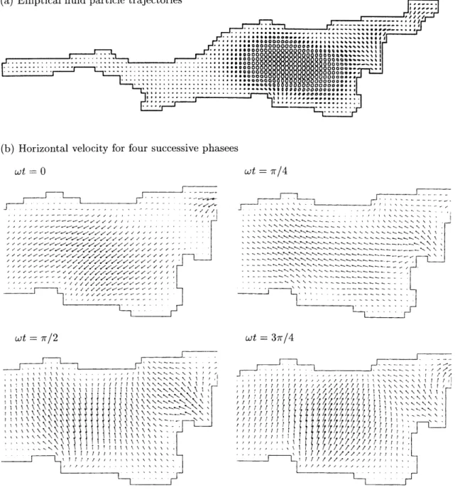
To give an example of the highly complex horizon-tal structure of the superinertial, PoincareÂ-type internal oscillations, we choose the twelfth mode (T ˆ11:9 h) of the two layer model which exhibits one well-developed, clockwise rotating amphidromic system situated at the broadest part of the basin (in the middle of the Upper Lake Constance). The horizontal structure of this mode, which is identi®ed by means of the ¯ow ellipses, and the corresponding horizontal velocity distributions for four successive phasesxtˆ0,

p=4, p=2, 3p=4 of the upper, those of the lower layer possess the rather similar structure, but in opposite direction. In Fig. 10a each ellipse represents a

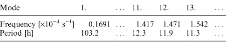
trajec-Table 1. Eigen frequencies and periods of the fundamental oscillation (1. mode) and three superinertial oscillations (11., 12. and 13. modes) subject to the strati®cation (2), which is replaced by a two-layer model witheˆ8:810 4_{,h1ˆ13 m andh2ˆh2…x;y†}

Mode 1. . . . 11. 12. 13. . . .

Frequency [´₁₀)4_s)1_{] 0.1691 . . . 1.417 1.471 1.542 . . .}

tory of a particle, which moves periodically around the centre of the respective ellipse. The size of the ellipses gives an indication of the excursion a particle encoun-ters. The clockwise veering of the current vectors in the central part of the basin is clearly seen from Fig. 10b± d. It is just the feature of the oscillation with the period of 12 h viewed in the time series of the wind-induced motion computed by the three-dimensional model (Fig. 8c).

From observations (Hollan, 1974; Heinz, 1995) we know that periods of approximately 12 h with clockwise veering currents are dominating the spectra at the centre of the Upper Lake Constance. This agrees with the twelfth mode of eigen oscillations of the two-layer numerical model. In general, PoincareÂ-type internal oscillations have smaller periods (always superinertial) the narrower the part of the basin where they occur. Here we only want to touch on observed short-period, free internal oscillations in the transverse direction of Lake UÈberlingen with periods of about 4 h, which Hollan (1974) explained as the response of strati®ed Lake UÈberlingen to local winds in the transverse direction. Calculations with a numerical two-layer model of high resolution (BaÈuerle, 1994) show that, in accordance with observations, the 4 h mode is restricted to the very end of Lake UÈberlingen. Further observa-tional evidence for this fact is given by Heinz (1995) in

extracting a 9-h period from the spectra of a measuring site between Lake UÈberlingen and the main basin of Upper Lake Constance. Such a wave should be found in a higher mode, it seems that the computation with higher resolution (near this domain) may be necessary.

Many other modes (e.g. 11.and 13. modes) of eigen oscillations possess complex structure and are hardly excited by uniform winds. Therefore, it seems that the fundamental subinertial Kelvin-type oscillation (1. mode) and the superinertial PoincareÂ-type oscilla-tions (e.g. 12. mode) can be easily excited by a spatially uniform wind. The other modes may occur under more complex wind distributions. Which of the superinertial PoincareÂ-type oscillations actually possesses relatively simple structure should depend on the value of the internal Rossby radius compared to the width of the basin. In the calculated three-dimensional wind-induced circulation in Sect. 3 these kinds of waves could indeed be easily identi®ed from the velocity ®eld. Their behaviour is the same as in the eigen oscillations: Kelvin-type oscillations circulate counter-clockwise around the basin and possess large amplitudes near the shore; PoincareÂ-type oscillations occur mainly in the centre of the basin and rotate in the clockwise direction. The periods of the oscillations estimated from the wind-induced circulations and the eigen oscillations basically coincide.

5 Concluding remarks

The internal response of medium-size lakes (as they exist in Alpine regions and other mountainous areas) to wind forcings is dominated by Kelvin and PoincareÂ-type wave dynamics. We have reported on the three-dimensional wind-induced baroclinic response of Lake Constance. Direct response to (simple) wind forcing and the oscillating behaviour after wind ceased were studied. It was demonstrated that this behaviour was well predict-ed. In particular, the dominant Kelvin- and PoincareÂ-type waves were reasonably reproduced, despite the fact that the attenuation is still somewhat larger than in real lakes of comparable size. The periods and features of the fundamental subinertial Kelvin-type wave, which is

shore-bound, and the three superinertial PoincareÂ-type waves, which occur mainly in the centre of the basin and whose periods increase (4 h, 9 h and 12 h) from left to right along the longitudinal direction with increasing basin width, were clearly identi®ed from the calculated three-dimensional wind-induced ¯ow ®eld. These peri-ods are well in accordance with the observations and the solutions of the eigenvalue problem.

The performance of the model can still be amended, i.e., di€usive mechanisms reduced, by using a larger number of Chebyshev polynomials; computations, how-ever, may become unduly long. The choice of the horizontal and (more so) vertical di€usivities is very crucial; in fact the velocity ®eld depends on the selection of the di€usivities. However, while our program allows

Fig. 10. aElliptical ¯uid particle trajectories andbthe corresponding horizontal velocities for four successive phases at 1/8cycle time intervals for the twelfth internal oscillation mode (PoincareÂ-type

to choose the values in the range that is thought to be physically acceptable, the vertical distribution and temporal variation can still not be chosen with sucient assurance of physical reliability. This dictates that the Reynolds-closure conditions must be computed along with the balances of mass, momentum and energy.

A step towards an improvement of this situation would be to add to these balance laws a closure condition of higher order, say by using an algebraic formula or one-parameter-closure scheme with a dif-ferential equation for the Reynolds stresses or a two-parameter-closure scheme with two di€erential equations, such as the k-e model. The former can be easily performed (see e.g. Svensson, 1978; Heaps, 1987; Rodi, 1993; Song and Haidvogel, 1994), however the latter still faces problems of instability under strong wind forcing, especially for three-dimensional modelling in lakes (see e.g. GuÈting, 1998; GuÈting and Hutter, 1998).

Acknowledgements. Topical Editor N. Pinardi thanks S. Pierini and J. O. Back-haus for their help in evaluating this paper.

References

BaÈuerle, E., Die Eigenschwingungen abgeschlossener, zweiges-chichteter Wasserbecken mit variabler Topographie,Rep.Inst. Meereskunde, Kiel,85,1981.

BaÈuerle, E.,Transverse baroclinic oscillations in Lake UÈberlingen, Aq.Sci.,56(2), 145±160, 1994.

BaÈuerle, E., D. Ollinger, and J. Ilmberger, Some meteorological, hydrological, and hydrodynamical aspects of Upper Lake Constance, in Eds. E. BaÈuerle and U. Gaedke,Lake Constance: characterisation of an ecosystem in transition, Arch. Hydrobiol. Spec. Issues Advanc. Limnol. 53, E. Schweizerbart'sche Ver-lagsbuchhandlung, Stuttgart, 31±83, 1998.

Bennett, J. R., A three-dimensional model of Lake Ontario's summer circulation, Part I: comparision with observations, J.Phys.Oceanogr.,7,591, 1977.

Chubarenko, B. V., Y. Wang, I. P. Chubarenko, and K. Hutter,

Simulation of wind-driven currents around a near-shore island by substructuring techniques. Island Mainau (Lake Constance) as an example.Ecol.Modell., in press, 1999.

GuÈting, P.,Dreidimensionale Berechnung windgetriebener StroÈmung mit einemk-e-Modell in idealisierten Becken und dem Bodensee, Shaker Aachen, ISBN 3-8265-3795-5, 343, 1998.

GuÈting, P., and K. Hutter, Modeling wind-induced circulation in the homogeneous Lake Constance using k-epsilon closure, Aq.Sci.,60,266±277, 1998.

Haidvogel D. B., and A. Beckmann, Numerical models of the coastal ocean,The Sea,10,1997.

Haidvogel, D. B., J. L. Wilkin, and R. Young, A semi-spectral primitive equation ocean circulation model using vertical sigma and orthogonal curvilinear horizontal coordinates,J.Comput. Phys.,94,151±185, 1991.

Heaps, N. S., Three-dimensional coastal ocean models, Coast. Estuar.Sci.,4,208, 1987.

Heinz, G., StroÈmungen im Bodensee. Ergebnisse einer Meûkam-pagne im Herbst 1993,Mitteil.VAW ETH ZuÈrich,135,237, 1995.

Hollan, E., StroÈmungsmessungen im Bodensee, Sechster Ber. AWBR,6,112±187, 1974.

Hollan, E., and T. J. Simons,Wind-induced changes of temperature and currents in Lake Constance, Arch. Meteorol Geophys. Bioklim.,Ser.A27,333±373, 1978.

Hutter, K., Fundamental equations and approximations, in Hydrodynamics of lakes, CISM-lectures, Ed. K. Hutter, Spring-er, Berlin Heidelberg, New York, 1984a.

Hutter, K., Mathematische Vorhersage von barotropen und baroklinen Prozessen im ZuÈrich- und Luganersee, Vier-jahresschr.Naturforsch.Ges.ZuÈrich,129,51±92, 1984b.

Hutter, K., G. Bauer, Y. Wang, and P. GuÈting, Forced motion response in enclosed lakes, Coastal and estuarine studies, 54,

137±166, 1998.

Lehmann, A.,A three-dimensional baroclinic eddy resolving model of the Baltic Sea,Tellus,47A,1013±1031, 1995.

Maiss, M., J. Ilmberger, A. Zenger, and K. O. MuÈnnich, A SF6

tracer study of horizontal mixing in Lake Constance,Aq.Sci.,

56(4), BirkhaÈuser Basel, 1994a.

Maiss, M., J. Ilmberger, and K. O. MuÈnnich, Vertical mixing in UÈberlingersee (Lake Constance) traced by A SF6 and heat,

Aq.Sci.,56(4), BirkhaÈuser Basel, 1994b.

Oman, G., Das Verhalten des geschichteten ZuÈrichsees unter aÈusseren Windlasten, Mitt. Versuchsans. Wasserbau, Hydrol. Glaziol.,ETH ZuÈrich,60,1982.

Peeters, F., Horizontale Mischung in Seen, Dissertation, ETH ZuÈrich, 1994.

Pohlmann, T.,A three dimensional circulation model of the South China Sea, in Eds. J. C. J. Nihoul and B. M. Jamart, Three-dimensional models of marine and estuarine dynamics, 245±268, 1987.

Ramming, H.-G., and Z. Kowalik,Numerical modelling of marine hydrodynamics. Elsevier Oceanography Series, 26, Elsevier Amsterdam, 368, 1980.

Rodi, W.,Turbulence models and their application in hydraulics±a state of the art review, A. A. Baalkema, Rotterdam, 104, 1993.

Simons, T. J.,Circulation models of lakes and inland seas, Can. Bull.Fish.Aq.Sci., 203, Ottawa, 1980.

Song, Y., and D. B. Haidvogel,A semi-implicit ocean circulation model using a generalized topography-following coordinate, J. Comput. Phy.,115,228±244, 1994.

Svensson, U.,A mathematical model of the seasonal thermpcline. University of Lund,Sweden,Rep.,1002,1978.

Tee, K.-T.,Simple models to simulate three-dimensional tidal and residual currents, in Ed. C. N. K. Mooers, Three-dimensional coastal ocean models,Coast.Est.Sci.,4,125±148, 1987.

Wang, Y., and K. Hutter,A semi-implicit semi-spectral primitive equation model for lake circulation dynamics and its stability performance,J.Comput.Phy.,139,209±241, 1998.

Wang, Y., and K. Hutter, Methods of substructuring in lake circulation dynamics,Adv.Water Resources,23,399±425, 2000.

Wilkin, J. L., J. V. Mansbridge, and K. Hedstrom,An application of the capacitance matrix method to accomodate masked land areas and island circulation in a primitive equation ocean model,Int.J.Num.Methods Fluids,20,649±662, 1995.