www.hydrol-earth-syst-sci.net/15/1167/2011/ doi:10.5194/hess-15-1167-2011
© Author(s) 2011. CC Attribution 3.0 License.
Earth System
Sciences
Regionalisation for lake level simulation – the case of Lake Tana in
the Upper Blue Nile, Ethiopia
T. H. M. Rientjes1, B. U. J. Perera2, A. T. Haile1, P. Reggiani3, and L. P. Muthuwatta4
1Department of Water Resources, Faculty of Geoinformation Science and Earth Observation (ITC), Twente University, P.O. Box 6, 7500 AA Enschede, The Netherlands
2National Water Supply and Drainage Board, Colombo, Sri Lanka 3DELTARES, P.O. Box 177, 2600 MH Delft, The Netherlands
4International Water Management Institute, P.O. Box 2075, Colombo, Sri Lanka
Received: 14 August 2010 – Published in Hydrol. Earth Syst. Sci. Discuss.: 27 September 2010 Revised: 18 March 2011 – Accepted: 21 March 2011 – Published: 8 April 2011
Abstract. In this study lake levels of Lake Tana are
simu-lated at daily time step by solving the water balance for all inflow and outflow processes. Since nearly 62% of the Lake Tana basin area is ungauged a regionalisation procedure is applied to estimate lake inflows from ungauged catchments. The procedure combines automated multi-objective calibra-tion of a simple conceptual model and multiple regression analyses to establish relations between model parameters and catchment characteristics.
A relatively small number of studies are presented on Lake Tana’s water balance. In most studies the water balance is solved at monthly time step and the water balance is simply closed by runoff contributions from ungauged catchments. Studies partly relied on simple ad-hoc procedures of area comparison to estimate runoff from ungauged catchments. In this study a regional model is developed that relies on principles of similarity of catchments characteristics. For runoff modelling the HBV-96 model is selected while multi-objective model calibration is by a Monte Carlo procedure. We aim to assess the closure term of Lake Tana’s water bal-ance, to assess model parameter uncertainty and to evaluate effectiveness of a multi-objective model calibration approach to make hydrological modeling results more plausible.
For the gauged catchments, model performance is as-sessed by the Nash-Sutcliffe coefficient and Relative Vol-umetric Error and resulted in satisfactory to good perfor-mance for six, large catchments. The regional model is vali-dated and indicated satisfactory to good performance in most
Correspondence to: T. H. M. Rientjes
cases. Results show that runoff from ungauged catchments is as large as 527 mm per year for the simulation period and amounts to approximately 30% of Lake Tana stream inflow. Results of daily lake level simulation over the simulation pe-riod 1994–2003 show a water balance closure term of 85 mm per year that accounts to 2.7% of the total lake inflow. Lake level simulations are assessed by Nash Sutcliffe (0.91) and Relative Volume Error (2.71%) performance measures.
1 Introduction
al. (2009) indicate that 42% of the lake inflow is from un-gauged systems. It is noted that closure of the lake water bal-ance in most studies (e.g. Kebede et al., 2006; SMEC, 2008) was by stream inflows from ungauged catchments. An actual closure term, however, could not be estimated and any error in one of the balance terms was compensated for by the esti-mate of the ungauged inflows. For estimation of the closure error of Lake Tana’s water balance, only in the work of (Wale et al., 2009) observed lake levels are compared to simulated lake levels by considering a detailed bathymetric survey.
Estimation of stream flow in ungauged basins commonly is based on principles of regionalisation which is the process of transferring information from gauged catchments to un-gauged catchment (see Bl¨oschl and Sivapalan, 1995). Merz and Bl¨oschl (2004) describe that regionalisation approaches may be based on similarity of spatial proximity or on simi-larity of catchment characteristics. The rationale of the first approach is that catchments of close proximity have a sim-ilar flow regime and therefore model parameters (MPs) are directly transferable. The rational for the second approach is that optimised MPs are transferable to other catchments in case the physical catchment characteristics (PCCs) are com-parable. Transferability is based on the idea that PCCs and (optimised) MPs values are related since, in their function-ing, parameters reflect on catchment characteristics. There-fore when establishing a relation between MPs and PCCs the information that is carried by the relation can be used to estimate parameter values from ungauged catchments when catchment characteristics from the ungauged systems are known. Regionalisation may serve to simply estimate stream flow from ungauged catchments but also serves to improve the predictive capability of the selected rainfall-runoff model by assessing model uncertainty. The need to improve the modeling of ungauged catchments is recognized by the In-ternational Association of Hydrologic Sciences (IAHS) by adopting the topic as one of the core components for their 10-yr Prediction in Ungauged Basins (PUB) project (see Siva-palan et al., 2003).
In Kebebe et al. (2006) and SMEC (2008) regionalisation procedures applied are based on similarity of spatial prox-imity principles and on simple comparisons of catchment sizes in the Lake Tana basin area. We note that in (Wale et al., 2009) both regionalisation procedures are applied but the similarity of catchment characteristics approach yielded best results where closure of Lake Tana balance was as ac-curate as 5.0% of the annual stream flow. This result must be considered the most accurate when compared to results by Kebebe et al. (2006); SMEC (2008) and the other above mentioned studies since the actual closure error of the water balance in those studies is not estimated by assessing how ac-curate observed lake levels are simulated. Therefore in those studies it remains unclear how well the lake water balance is represented.
The main objective of this study is to assess the closure term of Lake Tana’s water balance. Other objectives are to
assess model parameter uncertainty and to evaluate effec-tiveness of an automated multi-objective model calibration approach to make hydrological modeling results more plau-sible. For model calibration we selected a Monte Carlo sim-ulation procedure while performance assessments are based on the Nash Sutcliffe and Relative Volumetric Error objective functions. Validation of the procedure is by a split sample test. While the automated calibration procedure in this study is fundamentally different from the manual calibration proce-dure in Wale et al. (2009), different PCCs are tested and the representation lake evaporation has changed since estimation is now based on a more comprehensive satellite based proce-dure.
This paper is organised as follows. Descriptions of the study area and the availability data are given in Sects. 2 and 3 respectively. In Sect. 4 the hydrological model is presented. Section 5 describes the methodology that covers the cali-bration of the rainfall-runoff model, the configuration of the regional model and the simulation of water levels of Lake Tana. Section 6 presents and discusses the results of multi-objective model calibration, regionalisation and lake level simulation. In Sect. 7 conclusions are drawn.
2 Study area
Lake Tana (1786 m a.s.l.) is the source of the Blue Nile River and has a total drainage area of approximately 15 000 km2, of which the lake covers around 3000 km2. The lake is located in the north-western highlands of Ethiopia at 12◦00′N and 37◦15′E and receives runoff from more than 40 rivers. Major rivers feeding the lake are Gilgel Abay from the south, Ribb and Gumara from the east and Megech River from the north. From the western side of the lake only small river systems drain to the lake (Fig. 1).
Fig. 1. Gauged and ungauged catchments in the Lake Tana basin. Weather and gauge stations are indicated.
By its large size, Lake Tana has a large storage capacity that only responds slowly to the various processes of the cli-matic and hydrological cycles. Annual lake level fluctuations are approximately 1.6 m where lake level fluctuations pri-marily respond to seasonal influences by the rainy and the dry season. Lake levels reach maxima around September and minima around June with historic maximum and min-imum water levels of 1788.02 m (21 September 1998) and 1784.46 m (30 June 2003). The only river that drains Lake Tana is the Blue Nile River (Abay River) with a natural out-flow that ranges from a minimum of 1075 mm3 (1984) to a maximum of 6181 mm3 (1964). For the period 1976–2006 the average outflow is estimated to be 3732 mm3. For the se-lected simulation period, observations indicate that outflow of the lake was affected by operation of the Chara Chara weir from the end of 2001 onwards. Visual inspection of stream flow time series indicate that during the construction of the wear (1996–2001) Lake Tana outflow was not affected.
3 Data availability
From the National Meteorological Agency (NMA) in Ethiopia time series of daily rainfall from seventeen stations in and close to the study area were collected for the period of 1994–2003. Also from NMA, meteorological data was collected from seven weather stations for estimation of po-tential evapotranspiration. Data types are daily maximum and minimum temperature, wind speed, relative humidity and sunshine hours. From the database of the Hydrology Department of MoWR daily water levels of Lake Tana and
Soil classification resulted in 6 dominant soil classes. With regard to water storage capacity of Lake Tana, bathymetric relations between area-volume and elevation-volume were available through a bathymetric survey by the Faculty of Geoinformation Science and Earth observation, University of Twente, in 2005. The bathymetric relations were improved by Wale et al. (2009) by a more accurate delineation of the lake shore and are used in this study.
4 The HBV-96 model
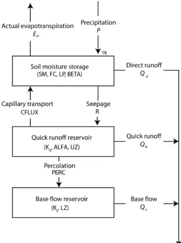
For stream flow simulation the HBV-96 model has been se-lected that has many applications in operational and strate-gic water management. Applications are known for lumped model domains (see Seibert, 1997) and semi distributed model domains (see Booij, 2005) and commonly aim at sim-ulating the rainfall-runoff relation. The model is classified as a conceptual water balance based model and relies on simple approximations to simulate mass exchange processes of the hydrological cycle. Input requirements to the model are pre-cipitation, temperature and potential evapotranspiration. In this study the HBV-96 model version (Lindstr¨om et al., 1997) is used with a simulation time step of one day. Four routines which are a precipitation accounting routine, a soil moisture routine, a quick runoff routine and a base flow routine are ac-tive and transform excess water from the soil moisture zone to local runoff (see Fig. 2).
The soil moisture routine controls the formation of direct and indirect runoff. Direct runoff occurs if the simulated soil moisture storage (SM), as conceptualised through a soil moisture reservoir representing the unsaturated soil, exceeds the maximum soil moisture storage denoted by parameter FC. Otherwise, all precipitation infiltrates (IN) the soil mois-ture reservoir, seeps through the soil layer or evapotranspires. The seepage through the soil layer causes indirect runoff (R)
that is determined through a power relationship with param-eter BETA as shown in Eq. (3) and the amount of infiltrating water and the soil moisture storage:
R = IN
SM
FC
BETA
. (1)
This indicates that indirect runoff increases with increas-ing soil moisture storage but also that indirect runoff reduces to zero in case infiltration becomes zero. Actual evapotran-spiration (Ea)depends on the measured potential evapotran-spiration (Ep), the soil moisture storage in the reservoir and a parameter LP which is a limit above which evapotranspira-tion reaches its potential value. This is shown in Eqs. (4) and (5).
Ea =
SM
LP·FC·Ep if SM < (LP·FC) (2)
Ea =Ep if SM ≥ (LP·FC) (3)
Fig. 2. A diagram of the HBV-96 approach (modified after Lind-str¨om, 1997).
At the quick runoff routine three components are distin-guished which are percolation to the base flow reservoir, capillary transport to the soil moisture reservoir and quick runoff. Percolation is denoted through parameter PERC which is a constant percolation rate that occurs when water is available in the quick runoff reservoir. Capillary trans-port is a function of the maximum soil moisture storage, the soil moisture storage and a maximum value for capillary flow (CFLUX) as shown in Eq. (6).
Cf = CFLUX·
FC
−SM FC
(4) If the yield from the soil moisture routine is higher than the percolation, then water becomes available for quick flow which is shown by Eq. (7).
Qq = Kq·UZ(1+ALFA) (5)
where UZ is the storage in the quick runoff reservoir, ALFA a measure for the non-linearity of the flow in the quick runoff reservoir andKqa recession coefficient.
The slow flow of the catchment is generated in the base flow routine through Eq. (8).
where LZ is the storage in the base flow reservoir andKs a recession coefficient.
5 Methodology
The regionalisation approach selected for this study encom-passes the following steps. First the HBV-96 model is cali-brated for gauged catchments against observed discharges to establish good performing parameters sets to simulate catch-ment runoff. Next, relationships are established between the model parameters (MPs) and Physical Catchment Character-istics (PCCs) to develop the so called “regional model”. This model is used to establish model parameters for ungauged catchments where MPs are defined based on the PCCs from the ungauged catchments. Then the HBV-96 model is used to simulate the runoff from the ungauged catchments. Finally, the water balance of Lake Tana is solved by considering all inflows and outflows and the closure term is calculated by comparing observed to simulated water levels. In the follow-ing subsections a description of the procedure is presented. A split sample test is applied to differentiate for periods of calibration (1994–2000) and validation (2001–2003) for the gauged catchments.
5.1 Model calibration
In this study model calibration is by a Monte Carlo Simu-lation (MCS) procedure. MCS is a technique where numer-ous model simulations are executed by randomly generated model parameter values with the objective to find the best performing parameter sets. Such set yields a minimum or maximum value for selected objective function(s). Good per-forming parameter sets are selected for further use and unsat-isfactory performing sets are denied for further use. Critical in MCS is the selection of the prior parameter space, the de-termination of the number of simulations to be executed and the selection of the objective function(s). For details on MCS simulation reference is made to Beven and Binley (1992); Harlin and Kung (1992) and Seibert (1999).
5.2 Parameter space
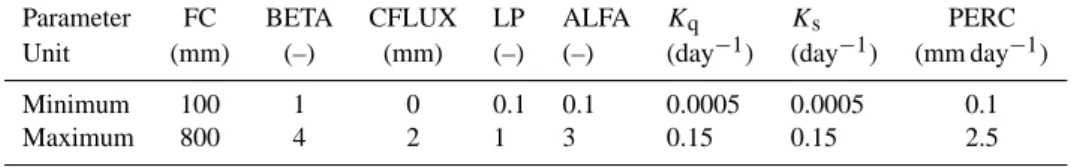
For selection of calibration parameters for MCS, a manual model sensitivity analysis is performed and literature on ap-plications of HBV-96 is reviewed. Studies for instance by Diermanse (2001), Lid´en and Harlin (2000), Seibert (1999) Hundecha and B´ardossy (2004) indicate model sensitivity to selected parameters. Selection of prior parameter space for MCS is based on studies by (Seibert, 1997; Booij, 2005; SMHI, 2006; de Vos and Rientjes, 2007; Wale et al., 2009). In Table 1 parameter ranges for selected parameters are given.
In MCS parameter values are randomly and independently sampled from uniform distributions. Principle to the valid-ity of MCS is that the entire parameter space is examined
to allow statistical evaluation of the results. Therefore, in this study we tested the performance of the model when the number of runs was systematically increased from 1000 to 100 000 and found that after 60 000 runs model performance could not be further improved. In the procedure the 10% of the best performing parameters sets are selected for further analysis. From this subset minimum and maximum parame-ter values for each parameparame-ter are defined and the MCS pro-cedure of 60 000 runs is repeated for the newly defined pa-rameter space. The optimally performing papa-rameter set now is defined by averaging the parameter values of the best per-forming 25 parameter sets. The procedure is applied to all gauged catchments and for each catchment an optimal pa-rameter set is defined. For assessing reliability of the param-eter estimates the entire MCS procedure is repeated 15 times and optimised parameter values for each of the catchments are compared. The comparison also is performed for single best parameter sets and serves to evaluate robustness of the procedure by comparing the averaged parameter values to the single best values.
5.3 Objective functions
In runoff model calibration the objective commonly is to op-timise parameter sets to match simulated stream flow to ob-served stream flow. Goodness of fit commonly is evaluated by visual inspection but also by use of objective functions that highlight selected aspects of the hydrograph such as low flows, high flows, the overall shape of a hydrograph or the rising limp of a hydrograph (see de Vos and Rientjes, 2007, 2008). Also the volumetric error is often addressed and in-dicates the mismatch between the volumes of runoff over the entire simulation period. In this work we selected two objec-tive functions that indicate the overall fit of the stream flow hydrograph and the volumetric errors. For the first objec-tive we selected the Nash-Sutcliffe (NS) efficiency criterion (Nash and Sutcliffe, 1970) and for the second objective we selected the Relative Volumetric Error (RVE). The NS ob-jective function requires maximisation and reads:
NS = 1−
n
P
i=1
(Qsim,i−Qobs,i)2 n
P
i=1
(Qobs,i−Qobs)2
(7)
whereQobsis mean of observed flow,Qsimis simulated flow,
Table 1. Prior parameter ranges.
Parameter FC BETA CFLUX LP ALFA Kq Ks PERC Unit (mm) (–) (mm) (–) (–) (day−1) (day−1) (mm day−1) Minimum 100 1 0 0.1 0.1 0.0005 0.0005 0.1
Maximum 800 4 2 1 3 0.15 0.15 2.5
is not straightforward and reference is made to Schaefli and Gupta (2007). The RVE requires minimisation and reads:
RVE =
n
P
i=1
Qsim,i−Qobs,i n
P
i=1
Qobs,i
×
100% (8)
RVE may range between−∞to +∞but indicates an excel-lent performing model when a value of 0 is generated. An error between +5% and −5% indicates a well performing model while error values between +5% and +10% or between
−5% and−10% indicate reasonable performance.
5.4 Selection of optimum parameter set
In the procedure of parameter set selection both objective functions are combined in a single objective function and performance of the model is assessed for the objective func-tion that suggest best model performance. The procedure is after Deckers et al. (2010) where four objective functions are combined. Comparatively, in this work we excluded NS ob-jective functions for high flows and low flows since results in Deckers et al. (2010) indicated that best performing parame-ter sets mostly are found by the NS or RVE objective func-tions. In the procedure for each parameter set both objective functions are calculated and compared. To evaluate which objective function indicates best performance, the value of each criterion was scaled over the range of objective function values by the 60 000 model runs. The NS value was scaled based on its minimum and maximum value:
CNS′ ,k,n = CNS,k,n−min(CNS,k,ntot)
max(CNS,k,ntot)−min(CNS,k,ntot)
(9)
whereCNSis value for the NS criterion,kindicates a specific catchment,nis calibration run number,ntotis run number.
Since RVE varies between−∞and +∞positive values as well as negative values can occur. The RVE scaling equation reads:
CRVE′ ,k,n=
CRVE,k,n
−max
CRVE,k,ntot
minCRVE,k,ntot
−max
CRVE,k,ntot
(10)
whereCRVEis value for the RVE criterion while other terms are as defined above.
After scaling of NS and RVE, the lowest value of the two was selected for each calibration run:
Ck,n′ =min{CNS′ ,k,n,CRVE′ ,k,n} (11)
whereC′is scaled value of the criteria.
The optimum parameter set for each catchment is now de-termined by selecting the highest values of all selected mini-mum values as determined through Eq. (14):
Ck=max{min(Ck,n′ tot)} (12)
It is noted that the procedure does not aim at selecting a pa-rameter set with a highest possible objective function value but aims to select a well performing parameter set by aver-aging over the 25 best performing sets. This procedure aims to prevent that outliers in parameter space may cause very high objective function values and refer to Beven and Bin-ley (1992) and Harlin and Kung (1992). Such parameter val-ues only have limited validity and must not be considered representative. Parameter values therefore are not suitable for establishing the regional model.
5.5 Establishing the regional model
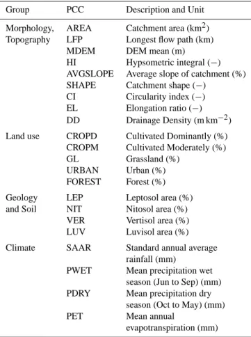
For developing a regional model the aim is to establish hy-drological relationships between MPs and PCCs. PCCs in this respect are characteristics of the catchment that relate to morphology, geometry, topography, climate, soils and land use. Selected PCCs should directly or indirectly affect the production of runoff in a catchment and as such selection is a critical step. In this work some 22 PCCs are selected from various sources. PCCs that relate to topography, geometry and the morphology of the catchments are extracted from the SRTM DEM. The PCCs under Land Use and Geology and Soil are obtained from the land use and soil map as described in Sect. 3. PCCs under Climate are from the meteorological data as made available by NMA. Table 2 shows the list of PCCs selected for this study.
Table 2. Selected physical catchment characteristics (PCCs).
Group PCC Description and Unit
Morphology, AREA Catchment area (km2) Topography LFP Longest flow path (km)
MDEM DEM mean (m)
HI Hypsometric integral (−) AVGSLOPE Average slope of catchment (%) SHAPE Catchment shape (−)
CI Circularity index (−) EL Elongation ratio (−) DD Drainage Density (m km−2) Land use CROPD Cultivated Dominantly (%)
CROPM Cultivated Moderately (%) GL Grassland (%)
URBAN Urban (%) FOREST Forest (%)
Geology LEP Leptosol area (%) and Soil NIT Nitosol area (%)
VER Vertisol area (%) LUV Luvisol area (%)
Climate SAAR Standard annual average rainfall (mm)
PWET Mean precipitation wet season (Jun to Sep) (mm) PDRY Mean precipitation dry
season (Oct to May) (mm) PET Mean annual
evapotranspiration (mm)
relationships of regional models in these studies are hydro-logically meaningful although relationships are statistically significant.
5.6 Regression analysis
Multiple linear regression is performed for each model pa-rameter. Statistical significance and strength are tested to guarantee that regression equations can be used. Also the correlation (r)is tested by the t-test (Eq. 15).
tcor=|
r|√n−2
√
1−r2 (13)
where,tcoristvalue of the correlation,ris correlation coef-ficient,nis sample size.
The following hypothesis is tested. The null hypothesis
H0and the specific hypothesisH1are:
H0: the correlation between the PCC and MPs is zero,
ρ=0.
H1: the correlation between the PCC and MPs is not zero,ρ6=0.
Iftcor> tcr the null-hypothesis is rejected (MPs are
associ-ated with PCCs in the population).
To determine the critical valuetcrthe number of degree of freedom, df, andα, a number between 0 and 1 to specify the confident level has to be determined. In this study a signifi-cant level ofα= 0.1 is chosen that is applied to a two-tail test withn-2 degree of freedom. Using this information, fortcra value of 2.132 is found (critical value fromt distribution ta-ble). To determine at whatrvalue the hypothesis is rejected the test statistic is solved. Anrof 0.72 was established and thusr greater than 0.72 and smaller than−0.72 results in a statistically significant relationship.
The second method applied is based on multiple regres-sion analysis to optimize the relationship with the forward selection and with the backward removal method. Multiple linear regression is used to predict MPs from several inde-pendent PCCs. In the forward entry approach the initially es-tablished regression model that incorporates the most signifi-cant PCC is extended by entering a second independent vari-able in the regional model. This step is accepted if the entry statistic (i.e. significance level,α) of both independent vari-ables is not exceeded. The statistical tools are used to select the independent variable that adds most significance to the relation. Additional steps are executed until the last added independent variable does not significantly contribute to the regression model. In addition to the forward entry method also the backward removal method is applied. In this method all expected PCCs are entered into the model. Based on the removal statistic (i.e. significance level,α) independent vari-ables are stepwise removed from the model. The significance of the multiple linear regression equations is tested by evalu-ating the significance of individual coefficients and by a test of overall significance. First a hypothesis test is applied to determine if the regression equation is significant. For such test it is assumed that the error term,ε, is not correlated and normally distributed. Further the error term must have an average of zero and a constant variance. In this study these assumptions are made and two hypothesis tests are executed to evaluate the significant of the regression equation. Those are the null-hypothesis and the specific hypothesis. Further the strength of the determined regression equation is evalu-ated by the coefficient of determination,r2.
5.7 Validation of the regional model
5.8 Lake level simulation
For simulation of daily lake level fluctuations the following water balance equation is solved:
1S
1T =P−Evap+Qgauged+Qungauged−QBNR (14)
where 1S/1T denotes the change in storage over time,
P is Lake areal rainfall, Evap is open water evaporation,
Qgaugedis Gauged river inflow,Qungaugedis Ungauged river inflow andQBNRis the Blue Nile River outflow (all terms in Mm3day−1).
For estimating lake evaporation the Penman-combination equation is selected where albedo was estimated us-ing the Moderate Resolution Imagus-ing Spectroradiometer (MODIS) Level 1b product (http://ladsweb.nascom.nasa. gov/data/search.html). Albedo is calculated from channels 1 to 7 by integrating band reflectance across the shortwave spectrum. Images require geometric, radiometric and spheric correction and the radiance at the top of the atmo-sphere needs to be known. During integration, weighting co-efficients are applied that represent the fraction of surface solar radiation occurring within the spectral range as rep-resented by a specific band. We refer to Liang (2001) and Liang et al. (2002) for extensive descriptions.
For the years 2000 and 2002 only some 14 and 16 cloud free images could be acquired, respectively. For days im-ages are not available, albedo values are estimated by in-terpolating albedo values between 2 subsequent acquisition days. Daily averaged values are defined by averaging the two albedo values and as such daily albedo maps are gen-erated for Lake Tana. A lake averaged albedo is estimated by averaging over all pixels that have spatial resolution of 1 km2. To estimate the lake evaporation, meteorological data from Bahir Dar station is used since out of the available sta-tions only this station is located close to Lake Tana. Daily rainfall over Lake Tana is estimated on daily base by spatial interpolation of gauge data from Bahir Dar, Chawhit, Zege, Deke Estifanos and Delgi station (see Fig. 1). We selected a weight power of 2 to allow representation of the relatively high spatial variability of rainfall in the basin (see Haile et al., 2009, 2010, 2011b).
For calculation of stream flow from gauged systems, ob-served stream flow time series are directly used in the water balance. Runoff time series are screened and corrected and analysis indicated that not all time series are reliable (see Sect. 3). For instance, results indicated that some gauges were relocated over time while other gauges indicated inun-dation during periods of extreme rainfall. For some gauges erroneous observations are identified by double mass curve analysis. Erroneous data is corrected by analyzing the ra-tio of incremental differences for consecutive days for rain-fall and runoff for the respective catchments. Outliers serve to identify errors and difference between consecutive rain-fall, or discharge observations serve to correct for erroneous
discharges or rainfall, respectively. The lake inflow from un-gauged systems is estimated by the regionalization approach as described in Sect. 5.2.
Time series for the Lake outflow by Abay River are di-rectly entered in the water balance equation after time series of outflow are corrected for consistency by use of a newly established stage-discharge relation in Wale et al. (2009).
In this study it is assumed that the groundwater system is decoupled from the lake and any lake leakage is ignored in the balance. We note that in (Kebede et al., 2006) lake leakage is estimated to be some 7% of the total annual lake budget. However, in Chebud and Melesse (2009), numeric groundwater modeling is applied and results indicate that lake leakage is unlikely and therefore exchange of water be-tween the lake and the groundwater system is ignored in the water balance calculations in this study.
6 Results and discussion
6.1 Gauged systems
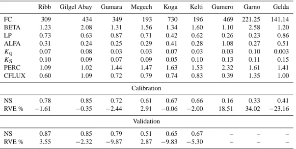
Results of MCS are shown in Table 3. For each of the catchments optimal parameter sets are identified and objec-tive function values for the optimized parameter set are cal-culated. Results of NS for calibration and validation in-dicate relatively high values for the 6 catchments with a highest calibration value of 0.85 for the Gilgel Abay catch-ment. The results of calibration are not satisfactory for Gumero (163 km2), Garno (98 km2)and Gelda (26 km2). All three catchments have low NS values (<0.41) while RVE values are relatively high. Therefore the use of these catch-ments is ignored when establishing the regional model. Wale et al. (2009) suggested that the time of concentration, which is defined as the time period for water to travel from the most remote point in the catchment to the outlet, is small. There-fore quick runoff responses often are not observed by the daily observations and also difficult to represent by the daily simulation time step. Further, some gauging stations are not placed at the catchment outlet but at a location upstream of the outlet that has easy road access. As such the runoff as observed does not indicate the catchment runoff and rainfall-runoff time series that are assumed to be representative for the respective catchments cannot be considered reliable since it is not clear which parts of the catchments are drained.
Table 3. Optimized model parameters for gauged catchments (1994–2000).
Ribb Gilgel Abay Gumara Megech Koga Kelti Gumero Garno Gelda
FC 309 434 349 193 730 196 469 221.25 141.14
BETA 1.23 2.08 1.31 1.56 1.34 1.60 1.10 2.58 1.20 LP 0.73 0.63 0.87 0.71 0.42 0.62 0.26 0.23 0.86 ALFA 0.31 0.24 0.25 0.29 0.41 0.28 1.08 0.27 0.51 Kq 0.07 0.08 0.03 0.03 0.07 0.03 0.03 0.10 0.003 KS 0.10 0.09 0.07 0.09 0.05 0.10 0.13 0.11 0.15 PERC 1.09 1.02 1.44 1.47 1.63 1.53 2.32 1.61 1.41 CFLUX 0.60 1.09 0.72 0.79 0.74 0.83 0.39 1.35 1.00
Calibration
NS 0.78 0.85 0.72 0.61 0.67 0.66 0.16 0.33 0.41 RVE % −1.61 −0.35 −2.44 2.91 −0.06 −2.00 18.51 34.02 −23.16
Validation
NS 0.87 0.85 0.79 0.51 0.65 0.67 – – –
RVE % 3.55 −2.32 −9.87 2.87 −9.83 −5.30 – – –
60 catchments; Young (2006) used 260 catchments for the entire UK; and Deckers et al. (2010) used 48 catchments also for the UK. To evaluate to what extent the small number of catchments in this study affected the regionalisation results is difficult and touches on the issue if a relatively large or small variability of catchment properties favours regionalisation. Little variation implies little hydrologic diversity and the de-velopment of robust regional model may be questioned while too much variability may result in weak relationships as sug-gested in (Young, 2006 and Deckers et al., 2010). Haber-landt et al. (2001) favour the assumption of large variability and a clear range of different conditions must be considered as a basis for regionalisation. Seibert (1999) and Wagener and Wheater (2006) on the other hand report on regionalisa-tion studies where catchments are characterised by relatively little variation. For the Lake Tana basin relatively high vari-ability of catchment properties is suggested in (Haile et al., 2009, 2011a), who indicated that large topographic variabil-ity directly affected the rainfall patterns. To asses variabilvariabil-ity we normalised PCC values for gauged and ungauged catch-ments by their area averaged values. Analysis indicates that normalised values of most PCCs for the gauged and the un-gauged catchments only change by some 20 to 30%. For the group of soils, normalised differences are large and range be-tween 0.02 and 5.84 while differences for climate PCCs are smallest with many values around 1.0 and a value range of 0.70–1.24. Larger differences are observed for the morpho-logic and topographic PCCs where most values are in be-tween 0.6 and 1.4 with value ranges 0.35–2.25. For land use related PCCs normalised values show largest variabil-ity but also values ranges are largest (i.e., between 0.01 and 6.41). Analysis of PCCs used in the regional model show a similar pattern. Morphology, topography and climate related
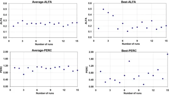
Fig. 3. Left hand side shows the average parameter values the 25 best performing parameter sets for ALFA and PERC for each MCS run of 60 000 runs each. The right hand side shows single best parameter values.
present average values of 25 best performing sets of 15 inde-pendent MCS runs, that a slightly different model structure is applied but also that slightly different prior parameter ranges are different. We further note that again different optimum values are found as compared to Abdo et al. (2009) and Wale et al. (2009) who applied manual calibration.
Figure 4 shows the Box and Whisker plots of parameters standardized by the prior range used for Monte Carlo Simu-lations (Gilgel Abay catchment). The boxes depict the me-dian and upper and lower quartiles. The whiskers indicate the most extreme values. The interquartile value ranges for ALFA are smallest and suggest that values are identified with consistency resulting in a stable region of solutions in pa-rameter space. We note that box values of the upper and lower quartiles are relatively small and suggest that small ALFA values favour a good performing model. The result also suggests high model sensitivity to ALFA and thus opti-mum values for the calibrations runs are well defined. FC shows relatively narrow interquartile box ranges and sug-gest that the model is quite sensitive to changes of FC. The remaining parameters have comparatively, equally large in-terquartile ranges and indicate lower sensitivity as compared to ALFA and FC. The whiskers indicate that distributions are not skewed and also suggest that the model is not highly sen-sitive. We note that ALFA is a measure for the non-linearity of the flow in the quick runoff reservoir while FC directly affects seepage flow and thus the quick runoff processes. Since both parameters affect the quick runoff behaviour of the model this indicates relatively low predictive uncertainty. Figure 5 shows the model calibration results of catch-ments used for developing the regional model. Table 3 also shows the model validation results for the period 2001–2003.
Fig. 4. Box and Whisker plots of parameters standardized by the prior range used for Monte Carlo Simulations (Gilgel Abay catch-ment). The boxes depict the median and upper and lower quartiles. The whiskers show the most extreme values.
Results for NS values in general slightly deteriorate as com-pared to the calibration results. RVE values in general are somewhat higher indicating larger errors in the water bal-ance. Errors for NS and RVE, however, are relatively small and indicate a good to satisfactory model performance of the regional model.
6.2 Regionalisation
0 100 200 300 400 Q ( m 3/s ) 0 20 40 60 80 100 120 P (mm ) Gilgel Abbay 0 50 100 150 200 250 300 Q ( m 3/s ) 0 20 40 60 80 100 120 P (mm ) Ribb 0 100 200 300 400 Q ( m 3/s ) 0 20 40 60 80 100 120 P (m m) Gum ara 0 20 40 60 80 100 Q ( m 3/s ) 0 20 40 60 80 100 120 P (m m) Megech 0 20 40 60 80 100
Apr-94 Apr-95 Apr-96 Apr-97 Apr-98 Apr-99 Apr-00
Q ( m 3 /s ) 0 20 40 60 80 100 120 P (m m) Koga 0 50 100 150 200
Apr-97 Apr-98 Apr-99 Apr-00
Time (days) Q ( m 3/s ) 0 20 40 60 80 100 120 P (mm )
P Qobs Qsim
Kelti
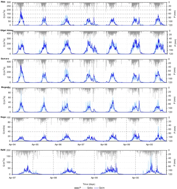
833
Fig. 5. Model calibration results of Ribb, Gilgel Abay, Gumara, Megech, Koga (1994–2000) and Kelti (1997–2000) catchments.
It is assumed that by use of multiple PCCs a better relation can be established than when only one PCC is used. There-fore relations between PCCs and MPs are assessed through multiple linear regression analysis. This is done by the for-ward entry method and the backfor-ward removal method as de-scribed in Sect. 5.2. The established regional model is shown in Table 5 and is followed by a description of each parameter. FC: in this study FC showed positive correlation with CI and negative correlation with HI and DD. The high-est correlation is with HI that is a measure of the distri-bution of elevation in a catchment and is defined as the average elevation a.m.s.l. minus the minimum divided by the difference between the maximum and minimum elevation a.m.s.l. The forward entry method was exe-cuted with HI as initial variable and results indicated
that there was no other variable that could improve the strength of the relation. Therefore the procedure was terminated and the regression equation is determined with only HI withR2 of 66.3%. The statistical char-acteristics are shown in Table 5. We note that from a hydrological perspective the relation between FC and HI may be questioned since FC reflects on soil prop-erties while HI reflects on catchment topography and geometry.
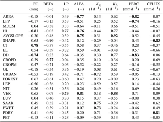
Table 4. Correlation matrix between model parameters and PCCs for 6 selected catchments; significant correlation coefficients are in bold.
FC BETA LP ALFA Kq KS PERC CFLUX (mm) (−) (−) (−) (1 d−1) (1 d−1) (mm d−1) (mm d−1) AREA −0.18 −0.01 0.49 −0.77 0.13 0.62 −0.82 0.07 LFP −0.17 −0.15 0.53 −0.51 0.25 0.52 −0.74 −0.16 MDEM 0.04 −0.58 0.33 −0.64 −0.11 0.66 −0.51 −0.51 HI −0.81 −0.03 0.77 −0.76 −0.44 0.77 −0.44 −0.07 AVGSLOPE −0.30 −0.48 0.39 −0.75 −0.31 0.92 −0.52 −0.45 SHAPE 0.65 −0.90 −0.42 0.12 −0.29 −0.04 0.43 −0.83 CI 0.78 −0.37 −0.55 0.58 0.37 −0.46 0.28 −0.37 EL 0.54 −0.59 −0.32 0.59 −0.01 −0.48 0.57 −0.66 DD −0.74 0.23 0.64 −0.35 0.30 0.77 −0.83 0.06 CROPD −0.39 0.77 −0.04 0.35 0.10 −0.36 0.20 0.69 CROPM 0.47 −0.71 0.03 −0.52 −0.22 0.27 −0.16 −0.55 GL −0.18 −0.54 0.36 −0.19 0.08 0.61 −0.42 −0.67 URBAN −0.53 −0.19 0.42 −0.71 −0.72 0.59 −0.05 −0.13 FOREST 0.67 −0.61 −0.60 0.47 0.20 −0.09 0.23 −0.63 LEP −0.50 −0.36 0.20 −0.23 −0.59 0.57 0.14 −0.44 NIT 0.26 −0.31 −0.56 0.26 −0.49 −0.16 0.69 −0.26 VER 0.65 0.07 −0.73 0.81 0.18 −0.88 0.71 0.09 LUV 0.04 0.40 0.30 0.15 0.37 −0.55 −0.08 0.38 SAAR 0.45 0.52 −0.31 0.12 0.75 −0.29 −0.42 0.62 PWET 0.45 0.39 −0.21 0.07 0.73 −0.24 −0.46 0.49 PDRY 0.41 0.69 −0.45 0.20 0.71 −0.36 −0.31 0.81 PET −0.13 −0.11 −0.23 −0.09 −0.59 0.13 0.43 −0.05
the square root of catchment size. Results of the for-ward entry method showed that BETA is correlated with SHAPE and HI withR2of 96.02%. From a hydrologi-cal point of view BETA can be related to both SHAPE and HI since BETA affects the generation of indirect runoff processes that relate to topographic characteris-tics. The statistical characteristics are shown in Table 5. LP: in this study the evapotranspiration parameter LP has significant positive correlation with HI and nega-tive correlation with VER that indicate poorly drained clay soils. The forward entry method is executed with highly correlated HI as the initial variable. This result showed that LP is correlated to HI and to LUV withR2
of 91.1%. LUV is % area luvisols that are active clays with medium to high water storage capacity. From a hy-drologic view point the relation between LP and LUV is much more plausible than the relation between LP and HI. The statistical characteristics are shown in Table 5. ALFA: in this study ALFA has positive correlation with VER and negative correlation with AREA (i.e., catch-ment area), HI and AVGSLOPE (i.e., average slope of catchment area). For optimisation of the relation the forward entry method is executed and yielded best re-sults with variable AREA as initial variable. We note that VER in all gauged catchments only is very small.
After adding the catchment characteristic URBAN (i.e., % urban area) theR2 increased up to 95.1% and this regression equation is accepted. Since ALFA is a quick runoff parameter this equation appears to be plausible. Catchments are of relative small size suggesting that runoff contributions by quick runoff are directly observ-able in the runoff hydrograph (i.e. not smoothened by long travel times) while a small % of urban area indi-cates small runoff contributions from paved areas. The statistical characteristics are shown in Table 5.
Kq: in this study the quick runoff recession coeffi-cient Kq showed correlation with URBAN (−0.72), SAAR (0.75) and PWET (0.73). The forward entry method is executed by taking SAAR (i.e., standard av-erage annual rainfall) as the initial variable. By adding other variables the strength could not be improved and the simple relation withR2of 56.35% is accepted. It is noted that the relation has no physical meaning since SAAR is a climate indicator on annual base. The statis-tical characteristics are shown in Table 5.
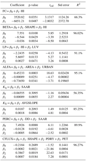
Table 5. The regional model and its statistical characteristics.
Coefficient p-value tcal Std error R2 FC=β0+β1·HI
β0 3520.82 0.0351 3.1317 1124.26 66.3% β1 −6651.21 0.0487 −2.8032 2372.70
BETA=β0+β1·SHAPE+β2·HI
β0 7.551 0.0100 5.85 1.2918 96.02% β1 −8.544 0.0429 −3.39 2.5233
β2 −0.036 0.0034 −8.50 0.0043 LP=β0+β1·HI+β2·LUV
β0 −2.2435 0.0258 −4.13 0.5432 91.1% β1 5.8697 0.0133 5.27 1.1141
β2 0.0027 0.0471 3.26 0.0008 ALFA=β0+β1·AREA+β2·URBAN
β0 0.45233 0.0003 18.63 0.02428 95.1% β1 −0.00009 0.0251 −4.17 0.00002
β2 −0.73650 0.0341 −3.71 0.19865 Kq=β0+β1·SAAR
β0 −0.06555 0.3095 −1.16 0.05636 56.35% β1 0.00009 0.0855 2.27 0.00004
KS=β0+β1·AVGSLOPE
β0 0.0187 0.2093 1.49 0.0125 85.25% β1 0.0018 0.0086 4.81 0.0004
PERC=β0+β1·DD+β2· SAAR
β0 7.4926 0.0088 6.11 1.2266 89.9% β1 −0.0128 0.0192 −4.61 0.0028
β2 −0.0005 0.0864 −2.52 0.0002 CFLUX=β0+β1·SHAPE+β2·PDRY+β3·PET
β0 −0.2184 0.2689 −1.52 0.1441 96.27% β1 −0.0082 0.0021 −21.86 0.0004
β2 0.3867 0.0019 22.63 0.0171 β3 0.0007 0.0184 7.28 0.0001
relation is accepted withR2of 85.25%. A recession co-efficient commonly relates to the catchment runoff re-sponse time where rere-sponse times commonly decrease when steepness increases. The statistical characteristics are shown in Table 5.
PERC: in this study PERC has negative relation with AREA (−0.82), LFP (−0.74) and DD (−0.83). The forward entry method was executed by adding DD (i.e., drainage density) as the first variable and after including SAAR,R2 increased up to 89.9%. From a hydrologi-cal context the equation may be plausible. A low DD commonly indicates that much rainfall in a catchment
is discharged by (delayed) groundwater flow where the groundwater domain is recharged by the percolation of rain water. PERC also may relate to SAAR where higher SAAR values may result in higher percolation values. The statistical characteristics are shown in Ta-ble 5.
CFLUX: in this study CFLUX has negative correla-tion with SHAPE (−0.83) and positive correlation with PDRY (0.81). Therefore optimisation of the linear re-lation with the forward entry method is executed with SHAPE as the initial variable. The results of the step-wise forward entry regression showed that CFLUX is correlated with SHAPE, PDRY (mean precipitation dry season) and PET (mean annual evapotranspiration) with
R2of 99.8%. Since capillary transport is triggered by atmospheric forcing the correlation of CFLUX to PDRY and to PET may be plausible. The correlation to SHAPE is not plausible. The statistical characteristics are shown in Table 5.
Results of the regression analysis for establishing the gional model indicate that statistically most significant re-gression equations can be obtained despite the fact that MPs can have low correlation to the selected PCCs (see Table 4). Obviously for such relations it is difficult to reason for hydro-logic plausibility. We note, however, that in litterateur (e.g. Deckers et al., 2010) more cases are known but also the use of PCCs with a high correlation not necessarily improve the regional model.
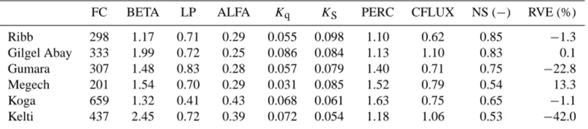
6.3 Performance assessment of the regional model
In most regionalisation studies, the validity of the regional model is assessed by its application to gauged catchments that are not used for establishing the regional model (see Sect. 5.7). Since in this work only a small number of gauged catchments is available, we used the regional model in Ta-ble 5 to estimate the model parameters for the gauged catch-ments using their PCCs. Simulated stream flow from the gauged catchments is compared to observed time series and assessments are by use of NS and RVE for the period 2001– 2003. Table 6 shows NS and RVE values and the parameter values as derived from the regional model. NS values range between 0.54 and 0.85 whereas RVE values range between
Table 6. Assessment of the regional model for gauged catchments (2001–2003).
FC BETA LP ALFA Kq KS PERC CFLUX NS (−) RVE (%) Ribb 298 1.17 0.71 0.29 0.055 0.098 1.10 0.62 0.85 −1.3 Gilgel Abay 333 1.99 0.72 0.25 0.086 0.084 1.13 1.10 0.83 0.1 Gumara 307 1.48 0.83 0.28 0.057 0.079 1.40 0.71 0.75 −22.8 Megech 201 1.54 0.70 0.29 0.031 0.085 1.52 0.79 0.54 13.3 Koga 659 1.32 0.41 0.43 0.068 0.061 1.63 0.75 0.65 −1.1 Kelti 437 2.45 0.72 0.39 0.072 0.054 1.18 1.06 0.53 −42.0
6.4 Lake level simulations
For lake level simulation all mass balance terms in Eq. (16) are solved on a daily time step and results of lake level simulations are compared to observed lake levels. As de-scribed in Sect. 5.3 for lake evaporation a procedure is ap-plied that combines the Penman-combination equation and a satellite based approach where albedo is estimated on a daily base to make up an annual cycle. Albedo ranged from 0.08 to 0.16 by the gradually changing solar zenith angle during the course of the year. Averaged daily evaporation is estimated at 4.6 mm day−1for the period 1992–2003 with a long-term averaged annual evaporation of 1563 mm yr−1. Minimum daily evapotranspiration is 2 mm day−1and max-imum is 6 mm day−1. Lake evaporation is lower than esti-mated in Wale et al. (2009) (1690 mm yr−1)but higher than in Kebebe et al. (2006) (1478 mm yr1). Daily rainfall over Lake Tana is estimated by spatial interpolation of gauge data from Bahir Dar, Chawhit, Zege, Deke Estifanos and Delgi station (Fig. 1). Inverse distance with power 2 resulted in an average lake precipitation of 1290 mm yr−1.
The results of lake level simulation are shown in Fig. 6 where simulated levels are compared to observed lake lev-els. The results indicate a good match where climatic sea-sonality with clear dry and wet periods is well presented. Largest deviations are observed specifically during the first few and last few years of the simulation period. Obvious rea-sons that cause the deviations are difficult to identify and can relate to any of the water balance terms. A quantitative as-sessment indicates that the balance closure term is as large as 85 mm yr−1of the total lake inflow that comprised rain-fall on the lake, and stream flow from gauged and ungauged catchments. This error accounts for 2.7% of the total lake inflow. In Wale et al. (2009) the closure error was−170 mm and accounted for 5% of the total lake inflow. In this work the smaller inflow error did not result in better lake level sim-ulation results when compared to Wale et al. (2009). Results of the lake level simulation are assessed by NS and RVE as well and resulted in values of 0.91 and−2.17%, respectively, whereas in Wale et al. (2009) NS was 0.90 and RVE was 1.6%.
Table 7. Lake Tana water balance components simulated for the period 1994–2003.
Water balance components mm yr−1 MCM yr−1 Lake areal rainfall +1347 +4104 Gauged river inflow +1254 +3821 Ungauged river inflow +527 +1605 Lake evaporation −1563 −4762 River outflow −1480 −4508
Closure term +85 +260
Compared to the work in Wale et al. (2009) differences in the annual lake balance are shown in Table 7. We note that refined procedures are applied in this work. For instance multi-objective model calibration by use of MCS is applied in this work, the procedure to estimate lake evaporation re-lies on daily varying albedo estimates and different PCCs are tested for regionalisation.
0 200 400 600 800
1/1/94 1/1/95 1/1/96 1/1/97 1/1/98 1/1/99 1/1/00 1/1/01 1/1/02 1/1/03
Q ( m 3/s ) Qgauged 0 200 400
1/1/94 1/1/95 1/1/96 1/1/97 1/1/98 1/1/99 1/1/00 1/1/01 1/1/02 1/1/03
Q ( m 3/s ) 600 Qungauged 0.0 20.0 40.0 60.0 80.0
1/1/94 1/1/95 1/1/96 1/1/97 1/1/98 1/1/99 1/1/00 1/1/01 1/1/02 1/1/03
P ( m m ) P 0.0 2.0 4.0 6.0 8.0 10.0
1/1/94 1/1/95 1/1/96 1/1/97 1/1/98 1/1/99 1/1/00 1/1/01 1/1/02 1/1/03
ET p ( m m ) ET 0 200 400 600 800
1/1/94 1/1/95 1/1/96 1/1/97 1/1/98 1/1/99 1/1/00 1/1/01 1/1/02 1/1/03
Time (days) Q ( m 3/s ) Qout 0 200 400 600 800
1/1/94 1/1/95 1/1/96 1/1/97 1/1/98 1/1/99 1/1/00 1/1/01 1/1/02 1/1/03
Q ( m 3/s ) Qgauged 0 200 400
1/1/94 1/1/95 1/1/96 1/1/97 1/1/98 1/1/99 1/1/00 1/1/01 1/1/02 1/1/03
Q ( m 3/s ) 600 Qungauged 0.0 20.0 40.0 60.0 80.0
1/1/94 1/1/95 1/1/96 1/1/97 1/1/98 1/1/99 1/1/00 1/1/01 1/1/02 1/1/03
P ( m m ) P 0.0 2.0 4.0 6.0 8.0 10.0
1/1/94 1/1/95 1/1/96 1/1/97 1/1/98 1/1/99 1/1/00 1/1/01 1/1/02 1/1/03
ET p ( m m ) ET 0 200 400 600 800
1/1/94 1/1/95 1/1/96 1/1/97 1/1/98 1/1/99 1/1/00 1/1/01 1/1/02 1/1/03
Time (days) Q ( m 3/s ) Qout
Fig. 6. Daily estimates of water balance terms of Lake Tana.
1782 1783 1784 1785 1786 1787 1788 1789
Apr-94 Apr-95 Apr-96 Apr-97 Apr-98 Apr-99 Apr-00 Apr-01 Apr-02 Apr-03
Time (days)
Observed Simulated
Fig. 7. Comparison of simulated to observed lake levels.
7 Conclusions
By availability of bathymetric relations, lake levels are sim-ulated on daily base over the simulation period. All water balance terms of Lake Tana are estimated explicitly and re-sults of lake level simulation showed NS of 0.91 and RVE of
−2.17%. Results of this study show that the Lake Tana wa-ter balance can be closed with a closure error of 85 mm yr−1 that accounts for 2.7% of the total lake inflow. Compared to previous studies on Lake Tana’s water balance by Setgen et al. (2005); SMEC (2008); Kebede et al. (2006); Chebud and Melesse (2009) and Wale et al. (2009) results of this study in-dicate smallest closure error. In this work probably the most
complete hydro-meteorological data set that is available for the basin is used. Runoff from gauged catchments is sim-ulated by use of a simple conceptual rainfall-runoff model and a Monte Carlo procedure. Model parameters for the un-gauged catchments are estimated by use of a regionalization procedure.
the selection of a different set of physical catchment charac-teristics as used for regionalisation. Multi-objective model calibration by use of MCS indicated that a very large num-ber of simulation runs must be executed. In this study a to-tal of 900 000 runs (i.e., 15×60 000 runs) is executed and resulted in relatively high parameter variability when single best parameter sets are defined for each of the 15 MCS runs but indicated moderate variability when averaged parameter values are compared for the 25 best performing parameter sets. Optimized parameter values in this study differ from Uhlenbrook et al. (2010) who used 1 000 000 runs for the Gilgel Abay catchment. Reasons for the difference could be that, instead of selecting the single best performing parame-ter set, we averaged the parameparame-ter values over 15 MCS runs were values over each run already represent averages over the 25 best performing sets. Also the selected prior param-eter ranges differ and a slightly different model structure is used. We note that manually calibrated parameter values in Wale et al. (2009) and Abdo et al. (2009) again differ.
Results of the regression analysis for establishing the re-gional model indicate that for all MPs statistically significant regression equations can be obtained. Relations, however, are not always plausible from a hydrological point of view. In this work it is shown that adding PCCs with high correla-tion to a regression relacorrela-tion not always results in an improved regional model. Out of the group of 22 PCCs only some 9 PCCs are used. PCCs most frequently used relate to topo-graphic, morphologic and climatic catchment settings.
Critical to the results of the regionalisation procedure in this work is the low number of gauged catchments. By the relatively small size of the Lake Tana basin only nine gauged catchments were available from which only six catchments had stream flow time series that could be used. We note that in most regionalisation studies a much larger set of gauged catchments is available (see Merz and Bl¨osch, 2004; Deckers at al., 2010; Young, 2006). Whether, however, the small set negatively affected our results is not entire clear. Validation results of the regional model in general do not suggest that the model should be rejected but also a normalization pro-cedure of PCCs for both gauged and ungauged catchments indicates that inter catchment variability does not constrain regionalization.
The use of remote sensing approach for estimating lake water albedo proved that albedo values over Lake Tana changed over the year by changing solar zenith angles. The use of satellite based albedo estimates resulted in lake evap-oration of 1563 mm yr−1. This value is lower than estimated in Wale et al. (2009) (1690 mm yr−1)but higher than in Ke-bebe et al. (2006) (1478 mm yr−1). Further assessments on the estimation of Lake Tana evaporation is required to better assess accuracy of the lake water balance. Such however is topic of ongoing research and a field campaign has been exe-cuted in 2009 with the aim to estimate lake evaporation by an energy balance method. For further assessments on the accu-racy of the water balance of Lake Tana we recommend that
extensive uncertainty analysis are performed for all balance terms. In this work we ignored such analysis and is left for future work. A simple analysis is already shown in Wale et al. (2009).
Acknowledgements. The three anonymous reviewers are gratefully acknowledged for their valuable comments on our manuscript. We also acknowledge the Ethiopian Meteorological Agency and the Ethiopian Ministry of Water Resources for their support by supplying the time series data for rainfall and stream flow. This study was financially supported by the Netherlands Fellowship Programme (NFP).
Edited by: T. Steenhuis
References
Abdo, K. S., Fiseha, B. M., Rientjes, T. H. M., Gieske, A. S. M., and Haile, A. T.: Assessment of climate change impacts on the hy-drology of Gilgel Abbay catchment in Lake Tana basin, Ethiopia, Hydrol. Process., 23(26), 3661–3669, 2009.
Bastola, S., Ishidaira, H., and Takeuchi, K.: Regionalisation of hydrological model parameters under parameter uncertainty: A case study involving TOPMODEL and basins across the globe, J. Hydrol., 357(3–4), 188–206, 2008.
Beven, K. and Binley, A.: The future of distributed models: model calibration and uncertainty prediction, Hydrol Process., 6, 279– 298, 1992.
Bl¨oschl, G. and Sivapalan, M.: Scale issues in hydrological mod-elling: a review, Hydrol Process., 9, 251–290, 1995.
Booij, M. J.: Impact of climate change on river flooding assessed with different spatial model resolutions, J. Hydrol., 303, 176– 198, 2005.
Chebud, Y. A. and Melesse, A. M.: Modelling lake stage and wa-ter balance of Lake Tana, Ethiopia, Hydrol. Process., 23, 3534– 3544, 2009.
Conway, D.: A water balance model of the Upper Blue Nile in Ethiopia, Hydrological Sciences Journal-Journal Des Sciences Hydrologiques, 42(2), 265–286, 1997.
Deckers, D. L. E. H., Booij, M. J., Rientjes, T. H. M., and Krol, M. S.: Catchment variability and parameter estimation in multi-objective regionalisation of a rainfall-runoff model, Water Re-sour. Manage., 24, 3961–3985, doi:10.1007/s11269-010-9642-8, 2010.
de Vos, N. J. and Rientjes, T. H. M.: Multi-objective performance comparison of an artificial neural network and a conceptual rainfall–runoff model, Hydrol. Sci. J., 52(1), 397–413, 2007. de Vos, N. J. and Rientjes, T. H. M.: Multi-objective training of
arti-ficial neural networks for rainfall–runoff modeling, Wat. Resour. Res., 44, W08434, doi:10.1029/2007WR006734, 2008. de Vos, N. J., Rientjes, T. H. M., and Gupta, H. V.: Diagnostic
eval-uation of conceptual rainfall–runoff models using temporal clus-tering, Hydrol. Process., 24, 2840–2850, doi:10.1002/hyp.7698, 2010.
Diermanse, F. L. M.: Physically based modelling of rainfall-runoff processes. PhD thesis, Delft University Press, Delft, 2001. Gupta, H. V., Wagener, T. Y., and Liu, Y.: Reconciling theory with
Haberlandt, U., Kl¨ocking, B., Krysanova, V., and Becker, A.: Re-gionalisation of the base flow index from dynamically simulated flow components – a case study in the Elbe River Basin, J. Hy-drol., 248, 35–53, 2001.
Haile, A. T., Rientjes, T. H. M., Gieske, M., and Gebremichael, M.: Rainfall Variability over mountainous and adjacent lake areas: the case of Lake Tana basin at the source of the Blue Nile River, J. Appl. Meteor. Climatol., 48, 1696–1717, 2009.
Haile, A. T., Rientjes, T. H. M, Gieske, A., and Gebremichael, M.: Rainfall estimation at the source of the Blue Nile: A multispec-tral remote sensing approach, Int. J. Appl. Earth Obs. Geoinf., JAG, 12, Supplement 1, S76–S82, 2010.
Haile, A. T., Rientjes, T. H. M., Gieske, A., Jetten, V., and Mekon-nen, G.: Satellite remote sensing and conceptual cloud modeling for convective rainfall simulation, Adv. Water Res., 34, 26–37, doi:10.1016/j.advwatres.2010.08.007, 2011a.
Haile, A. T., Rientjes, T. H. M., Habib, E., Jetten, V., and Ge-bremichael, M.: Rain event properties at the source of the Blue Nile River, Hydrol. Earth Syst. Sci., 15, 1023–1034, doi:10.5194/hess-15-1023-2011, 2011b.
Harlin, J. and Kung, C.: Parameter uncertainty and simulation of design floods in Sweden, J. Hydrol., 137, 209–230, 1992. Heuvelmans, G., Muys, B., and Feyen, J.: Regionalisation of the
parameters of a hydrological model: Comparison of linear re-gression models with artificial neural nets, J. Hydrol., 319(1–4), 245–265, 2006.
Hundecha, Y. and B´ardossy, A.: Modeling of the effect of land use changes on the runoff generation of a river basin through param-eter regionalization of a watershed model, J. Hydrol., 292(1–4), 281–295, 2004.
Kebede, S., Travi, Y., Alemayehu, T., and Marc, V.: Water balance of Lake Tana and its sensitivity to fluctuations in rainfall, Blue Nile basin, Ethiopia, J. Hydrol., 316(1–4), 233–247, 2006. Kim, U., Kaluarachchi, J. J., and Smakhtin, U.: Generation of
monthly precipitation under climate change for the Upper Blue Nile river basin Ethiopia, J. Am. Water Resour. As., 44(2), 1–17, doi:10.1111/j.1752-1688.2008.00220.x., 2008.
Klemeˇs, V.: Operational testing of hydrological simulation models, Hydrol. Sci. J., 31, 13–24, 1986.
Liang, S.:. Narrowband to broadband conversions of land surface albedo: I. Formulae, Remote Sens. Environ., 76, 213– 238, 2001. Liang, S., Shuey, C., Russ, A., Fang, H., Walthall, C., and Daugh-try, C.: Narrowband to broadband conversions of land surface albedo: II. Validation, Remote Sens. Environ., 84, 25–41, 2002. Lid´en, R. and Harlin, J.: Analysis of conceptual rainfall-runoff
modelling performance in different climates, J. Hydrol., 238, 231–247, 2000.
Lindstr¨om, G., Johansson, B., Persson, M., Gardelin, M., and Bergstr¨om, S.: Development and test of the distributed HBV-96 hydrological model, J. Hydrol., 201, 272–288, 1997.
Merz, R. and Bl¨oschl, G.: Regionalisation of catchment model pa-rameters, J. Hydrol., 287, 95–123, 2004.
Nash, J. E. and Sutcliffe, J. V.: River flow forecasting through con-ceptual models, Part I. A discussion of principles, J. Hydrol., 10, 282–290, 1970.
Rientjes, T. H. M., Haile, A. T., Mannaerts, C. M. M., Kebede, E., and Habib, E.: Changes in land cover and stream flows in Gilgel Abbay catchment, Upper Blue Nile basin - Ethiopia, Hy-drol. Earth Syst. Sci. Discuss., 7, 9567–9598, doi:10.5194/hessd-7-9567-2010, 2010.
Schaefli, B. and Gupta, H. V.: Do Nash values have value?, Hydrol. Process., 21, 2075–2080, doi:10.1002/hyp.6825, 2007.
Sefton, C. E. M. and Howarth, S. M.: Relationships between dy-namic response characteristics and physical descriptors of catch-ments in England and Wales, J. Hydrol., 211, 1–16, 1998. Seibert, J.: Estimation of parameter uncertainty in the HBV model,
Nordic Hydrol., 28, 4–5, 1997.
Seibert, J.: Regionalisation of parameters for a conceptual rainfall-runoff model, Agr. Forest Meteorol., 98–99, 279–293, 1999. Setegn, S. G., Srinivasan, R., and Dargahi, B., Hydrological
Mod-elling in the Lake Tana Basin, Ethiopia Using SWAT Model, The Open Hydrology Journal, 2, 49–62, 2008.
Sivapalan, M., Takeuchi, K., Franks, S. W., Gupta, V. K., Karam-biri, H., Lakshmi, V., Liang, X., McDonnell, J. J., Mendiondo, E. M., O’Connell, P. E., Oki, T., Pomeroy, J. W., Schertzer, D., Uhlenbrook, S., and Zehe, E.: IAHS Decade on Predictions in Ungauged Basins (PUB), 2003–2012: Shaping an exciting fu-ture for the hydrological sciences, Hydrol. Sci. J., 48, 857–880, 2003.
SMEC: Hydrological Study of the Tana-Beles sub-basins, main report, Snowy Mountains Engineering Corporation, Australia, 2008.
SMHI: Integrated Hydrologic Modelling System (IHMS), Manual version 5.1., 2006.
Uhlenbrook, S., Mohamed, Y., and Gragne, A. S.: Analyzing catch-ment behavior through catchcatch-ment modeling in the Gilgel Abay, Upper Blue Nile River Basin, Ethiopia, Hydrol. Earth Syst. Sci., 14, 2153–2165, doi:10.5194/hess-14-2153-2010, 2010. Wagener, T. and Wheater, H. S.: Parameter estimation and
region-alization for continuous rainfall-runoff models including uncer-tainty, J. Hydrol., 320, 132–154, 2006.
Wale, A., Rientjes, T. H. M., Gieske, A. S. M., and Getachew, H. A.: Ungauged catchment contributions to Lake Tana’s water balance, Hydrol. Process., 23(26), 3682–3693, 2009.
Xu, C.: Testing the transferability of regression equations derived from small sub-catchments to a large area in central Sweden, Hy-drol. Earth Syst. Sci., 7, 317–324, doi:10.5194/hess-7-317-2003, 2003.