www.atmos-chem-phys.net/9/1303/2009/ © Author(s) 2009. This work is distributed under the Creative Commons Attribution 3.0 License.
Chemistry
and Physics
Increasing ozone in marine boundary layer inflow at the west coasts
of North America and Europe
D. D. Parrish1, D. B. Millet2, and A. H. Goldstein3
1NOAA Earth System Research Laboratory, Chemical Sciences Division, 325 Broadway R/CSD7, Boulder, CO 80305, USA 2Department of Soil, Water & Climate, University of Minnesota, St. Paul, MN, USA
3Department of Environmental Science, Policy, and Management, University of California, Berkeley, CA, USA
Received: 9 June 2008 – Published in Atmos. Chem. Phys. Discuss.: 22 July 2008 Revised: 26 January 2009 – Accepted: 26 January 2009 – Published: 19 February 2009
Abstract. An effective method is presented for determin-ing the ozone (O3) mixing ratio in the onshore flow of
ma-rine air at the North American west coast. By combining the data available from all marine boundary layer (MBL) sites with simultaneous wind data, decadal temporal trends of MBL O3 in all seasons are established with high
preci-sion. The average springtime temporal trend over the past two decades is 0.46 ppbv/yr with a 95% confidence limit of 0.13 ppbv/yr, and statistically significant trends are found for all seasons except autumn, which does have a significantly smaller trend than other seasons. The average trend in mean annual ozone is 0.34±0.09 ppbv/yr. These decadal trends at the North American west coast present a striking comparison and contrast with the trends reported for the European west coast at Mace Head, Ireland. The trends in the winter, spring and summer seasons compare well at the two locations, while the Mace Head trend is significantly greater in autumn. Even though the trends are similar, the absolute O3mixing ratios
differ markedly, with the marine air arriving at Europe in all seasons containing 7±2 ppbv higher ozone than marine air arriving at North America. Further, the ozone mixing ra-tios at the North American west coast show no indication of stabilizing as has been reported for Mace Head. In a larger historical context the background boundary layer O3mixing
ratios over the 130 years covered by available data have in-creased substantially (by a factor of two to three), and this increase continues at present, at least in the MBL of the Pa-cific coast region of North America. The reproduction of the increasing trends in MBL O3over the past two decades, as
well as the difference in the O3 mixing ratios between the
Correspondence to:D. D. Parrish (david.d.parrish@noaa.gov)
two coastal regions will present a significant challenge for global chemical transport models. Further, the ability of the models to at least semi-quantitatively reproduce the longer-term, historical trends may an even greater challenge.
1 Introduction
Reliably establishing the temporal trends of background O3
in the northern mid latitudes is very important to our under-standing of the budget of tropospheric O3. (Here we use the
term “background O3” to qualitatively describe O3 mixing
ratios measured at a given site in the absence of strong lo-cal effects. Different publications have used different quan-titative definitions; in the following sections we develop the quantitative definition used in this work.) The majority of anthropogenic precursors of O3are emitted at northern mid
latitudes, and these emissions have increased over the last century, most dramatically beginning around 1950 (van Aar-denne et al., 2001). This increase began first over North America and Europe, and more recently has accelerated over Asia. In about 1970 emissions from Europe and North Amer-ica began to stabilize and since have decreased (RETRO, 2007). This decrease has been significantly more rapid for volatile organic carbon species than for the oxides of nitro-gen, particularly in North America. In contrast emissions from Asia continue to increase (RETRO, 2007). The ability of global chemical transport models to reproduce changes in tropospheric O3that have occurred in response to these
and aerosols. However, for such tests to achieve maximum success it is critical that analyses of field observations char-acterize the temporal trends of the tropospheric O3 mixing
ratios as accurately and precisely as possible.
Establishing the temporal trends and the absolute magni-tude of background O3is also important from the perspective
of local and regional air quality control. The O3transported
into a region determines how much locally produced O3can
be added before exceeding air quality standards. As peak O3
is decreased due to local and regional air pollution control measures, the background O3becomes even more important
when considering the potential efficacy of future air pollution control measures. Also, increasing background O3can
off-set the benefits of these local and regional control measures (e.g., Jacob et al., 1999).
The earliest trend analyses of O3 that were based upon
techniques thought to yield reliable results (Volz and Kley, 1988; Staehelin et al., 1994) indicated that O3increased by
at least a factor of two in near-surface air at suburban to re-mote regions of Europe between the late 1800s and the early 1980s. There is concern regarding the confidence that can be placed in these early measurements, but considerable ef-fort was put into maximizing this confidence. More recent trend analyses, as summarized by Oltmans et al. (2006), have found significant regional differences, and no consistent in-crease or dein-crease in tropospheric O3has been established,
particularly for the northern mid latitudes.
Over continents competing effects make it difficult to char-acterize background O3. Fiore et al. (2002) conclude that
over North America the observed decrease in the high end of the O3probability distribution in surface air over the United
States reflects reduction of domestic hydrocarbon emissions, while the increase in the low end reflects, at least in their model, rising Asian emissions. The O3trends over the 1987–
2004 time period at nine rural sites in the western continen-tal United States (Jaffe and Ray, 2007) varied between 0 and 0.51 ppbv/yr with a statistically significant positive trend at seven of the nine sites. The impact of transport events bring-ing diluted plumes of urban origin with O3from the high end
of the probability distribution likely varies between the nine sites, and thus plays a significant role in the large variability in these temporal trends. One goal of the present analysis is to avoid the impact of transported plumes of O3produced
locally in order to characterize the temporal trend of back-ground O3transported into the region.
Two particularly important locations to characterize O3
trends are at the downwind side of the North Pacific and North Atlantic Oceans. These downwind locations receive air representing a regional integration over outflow from wide regions of the upwind continents. The O3mixing
ra-tios in continental outflow are modified by the interaction of transport, mixing and O3 production and loss processes
during transport through the marine environment. With only limited emission sources and minimal O3deposition within
the marine environment, mixing and chemical processes tend
to reduce the variability of the marine O3. The observed
vari-ability of O3in marine air received on the downwind coast
largely reflects variability of large-scale flow patterns of the transported air masses. Measurements within the marine air inflow also provide the potential to sample O3in an
environ-ment without dominant confounding continental influences such as in situ O3production from locally emitted
precur-sors, transport of air masses with widely varying histories, surface deposition, reaction of O3with local emissions, etc.
Temporal changes in these influences undoubtedly contribute to the significant regional differences found in O3trends at
northern mid latitudes (Oltmans et al., 2006; Jaffe and Ray, 2007). If trends in background O3 can be established for
the downwind sides of the two large oceans at northern mid latitudes, then they are likely of more fundamental impor-tance to our understanding of the background tropospheric O3budget than are the variable regional trends over the
con-tinents. However, to characterize these marine trends from land surface based measurements requires careful discrimi-nation against continental effects in the analysis of the avail-able data sets. Our goal in this paper is to characterize these temporal trends in the boundary layer of these two marine environments.
Investigators have presented evidence that the background O3 has increased since the mid-1980s at northern mid
lat-itudes in air entering both the North American west coast form the North Pacific Ocean (Jaffe et al., 2003; Parrish et al., 2004a) and the European west coast from the North At-lantic Ocean (Simmonds et al., 2004; Derwent et al., 2007). Parrish et al. (2004a) argue that the increase in the North Pacific has occurred in response to increasing Asian emis-sions of O3precursors, which are transported to the North
Pacific troposphere. However, other investigators (Oltmans et al., 2006, 2008) have suggested that the reported increase at the North American west coast was actually caused by lo-cal North American continental effects rather than represent-ing an increase in the background marine O3. A resolution
to this disagreement is important for establishing the confi-dence that can be attached to the reported marine O3trends.
In an effort to reach a resolution of this disagreement, the first goal of this paper is to comprehensively review the available observations and analyses that provide the basis for determining the O3 temporal trend at the North American
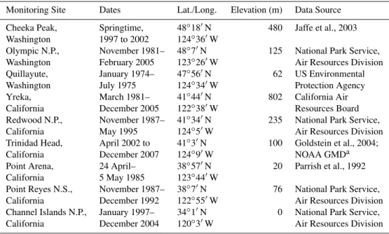
Table 1.Ozone data sets investigated in the present analysis.
Monitoring Site Dates Lat./Long. Elevation (m) Data Source Cheeka Peak, Springtime, 48◦18′N 480 Jaffe et al., 2003 Washington 1997 to 2002 124◦36′W
Olympic N.P., November 1981– 48◦7′N 125 National Park Service, Washington February 2005 123◦26′W Air Resources Division Quillayute, January 1974– 47◦56′N 62 US Environmental Washington July 1975 124◦34′W Protection Agency Yreka, March 1981– 41◦44′N 802 California Air California December 2005 122◦38′W Resources Board Redwood N.P., November 1987– 41◦34′N 235 National Park Service, California May 1995 124◦5′W Air Resources Division Trinidad Head, April 2002 to 41◦3′N 100 Goldstein et al., 2004; California December 2007 124◦9′W NOAA GMDa Point Arena, 24 April– 38◦57′N 20 Parrish et al., 1992 California 5 May 1985 123◦44′W
Point Reyes N.S., November 1987– 38◦7′N 76 National Park Service, California December 1992 122◦55′W Air Resources Division Channel Islands N.P., January 1997– 34◦1′N 0 National Park Service, California December 2004 120◦3′W Air Resources Division
aNational Oceanic and Atmospheric Administration, Earth System Research Laboratory, Global Monitoring Division
goal to carefully examine trends in all seasons, and to eval-uate the suggestions of Oltmans et al. (2006, 2008) that the previously derived trends do not represent the marine tropo-sphere. We find results here that are fully consistent with the conclusions presented by Jaffe et al. (2003) and Parrish et al. (2004a), with the statistical confidence considerably im-proved. It is shown that the data sets on which Oltmans et al. (2006, 2008) based their suggestions have serious short-comings. A future paper will examine data from higher el-evation, inland sites that receive direct inflow of marine air, including Lassen Volcanic National Park, and data sets col-lected from aircraft and sondes; preliminary analysis of these data supports the trends found by Jaffe et al. (2003) and Par-rish et al. (2004a) as well.
The second goal of this paper is to place the derived North American west coast MBL O3trends into a larger spatial and
historical context by comparing them with reported Euro-pean tropospheric O3 trends. An increasing trend over the
past two decades has been well established at Mace Head, Ireland (Simmonds et al., 2004; Derwent et al., 2007). We will show that the trends of MBL O3 at the west coast of
North America have some marked similarities to and marked differences from these European trends.
This paper is organized as follows. Section 2 reviews all of the MBL O3data that have been collected on the North
American west coast and that have been suggested as suit-able for characterizing background O3. Section 3 discusses
in detail the analysis that is required to characterize marine O3from measurements conducted at land-based sites
receiv-ing direct MBL inflow. Section 4 derives the North
Ameri-can temporal O3trends for each season, and Sect. 5 examines
systematic variations in the O3including seasonal and
diur-nal cycles and dependence upon a particular air mass flow regime. Finally, Sect. 6 discusses the significance of the de-rived O3trends in the context of the European data sets.
2 Available North American marine boundary layer data sets
To our knowledge, O3 measurements have been reported
from eight, near-sea level sites on the west coast of North America that have been identified as suitable for character-izing O3 in marine air inflow to the continent. Table 1 and
Fig. 1 identify site locations, the dates of O3measurements
investigated here, some site characteristics and the source of the data. These eight sites include the five sites discussed by Jaffe et al. (2003) and Parrish et al. (2004a) (Cheeka Peak in Washington and Redwood N.P., Trinidad Head, Point Arena, and Point Reyes N.S. in California), two sites suggested by Oltmans et al. (2006, 2008) (Olympic N.P in Washington and Channel Islands N.P. in California) and Quillayute, Washing-ton where some very early measurements were made (Singh et al., 1978). Also included in Table 1 and Fig. 1 is an inland, continental boundary layer site (Yreka, California) that Olt-mans et al. (2006, 2008) suggest is useful for characterizing the marine background O3flowing into North America.
Most of the O3 measurements at these sites were made
Cheeka Peak
Pt. Reyes NS
Olympic NP
Yreka
Quillayute
Redwood NP
Trinidad Head
Pt. Arena
Channel Is.
NP
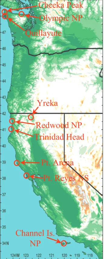
Fig. 1.Map of the North American west coast showing location of surface sites from which the data sets discussed were collected. The colors indicate terrain topography.
Laboratory of the National Oceanic and Atmospheric Ad-ministration (NOAA GMD) have each employed a consis-tent calibration procedure based on US EPA methods. The Pt. Arena field study followed careful data validation proce-dures. Generally the O3 data sets are believed to be
accu-rate to within±3%, and the one-hour average data used in this analysis precise to within±2% or 1 ppbv, whichever is greater. One exception to these limits of accuracy and preci-sion is the earliest data set collected in the mid-1970s at Quil-layute, Washington. These are the only measurements that were made using a chemiluminescence technique, and these measurements were made before the US EPA promulgated regulations that defined procedures and approved reference or equivalent methods. Therefore these data are of uncertain quality, and will not be examined in detail. Further, some of the early data from Olympic N.P. were collected by national park staff before the NPS Air Resources Division established the full quality assurance program. Thus, the early data from Olympic N.P. will be examined only with appropriate reser-vations.
One significant instrumental problem has been identified in the available data sets. NPS personnel report that at the Olympic NP site, the instrument sampling system evidently leaked substantially during the period between maintenance visits on 7 March 2002 and 23 January 2003. Data collected during this period have been eliminated from further consid-eration.
3 Analysis of data
Characterizing O3 in the MBL from measurements
con-ducted at land-based sites presents significant challenges since the measurements necessarily must be conducted in an environment with at least some air-land surface influence. This influence significantly affects the observed ambient O3
through deposition to the ground and other surfaces (most importantly vegetation), O3destruction by reaction with
lo-cal emissions, and photochemilo-cal O3 production from
pre-cursors emitted from land-based sources or even from within the near coastal marine environment (e.g. emissions from coastal shipping lanes.) It is critical that the significance of such effects be investigated, and if significant, their influence eliminated, or at least minimized, in the data sets considered. Elimination of land effects is most straightforward at is-land sites. Measurements have been reported from several such sites in the temperate North Atlantic: Bermuda, Barba-dos, and Westman Island, Iceland (Oltmans and Levy, 1994); Sable Island and Seal Island, Canada (Parrish et al., 1998); and the Azores (Parrish et al., 1998; Honrath et al., 2004). On islands as small and well ventilated as Sable Island (approxi-mately 1 km wide, by 40 km long; mean winds usually 10 to 20 m/s) undisturbed marine O3is generally always sampled
to isolate the marine signature (e.g. Oltmans and Levy, 1994). Measurements have not been made at comparable island sites in either the eastern North Pacific or eastern North Atlantic, so measurements at coastal, continental sites provide the only land-based approach for characterization of marine O3near
the North American and European coasts. Coastal sites are more appropriate at the west coasts of North America and Europe than at the east coast of a continent, since the prevail-ing westerly winds assure the prevalence of onshore flow of marine air.
Even with the prevailing onshore flow at the west coasts of North America and Europe, there are synoptic and smaller scale circulation patterns that transport continentally influ-enced air into the marine environment. To determine trends in marine O3it is important to screen out measurements that
are significantly affected by continental effects. At the Mace Head, Ireland site, both “pollution filtering” and air mass ori-gin as determined from a Lagrangian dispersion model (Sim-monds et al., 2004; Derwent et al., 2007) have been shown to be effective for removing continentally influenced data. Here we will simply take the monthly mean O3 data from Mace
Head, Ireland (Table 1 of Derwent et al. (2007)) that was se-lected as baseline air. However, at the North American west coast, complex small-scale circulation patterns, driven both by temperature gradients between the marine and continental environment and by orographic features of the coastal zone, can transport continentally influenced air into the marine en-vironment and can mix air into the MBL from the lower free troposphere. These circulation patterns are likely much more important at the North American west coast than in Europe due to the stronger land-sea temperature gradients and the larger orographic features on the North American coast. Here we will examine effective means for eliminating the con-tinentally influenced measurements at the North American west coast.
3.1 Selection of marine air by trace species measurements The dependence of O3mixing ratios on meteorological
vari-ables and the correlation of O3 mixing ratios with those of
other trace species provide two means of identifying conti-nental effects. Trinidad Head is the North American west coast site with the most extensive trace gas measurements (Goldstein et al., 2004; Millet et al., 2004) made during the five-week ITCT 2K2 field study in the spring of 2002 (Parrish et al., 2004b). Continuous measurements of O3and
meteoro-logical variables have been maintained there since that time (Oltmans et al., 2008), and it is also a site included in the Advanced Global Atmospheric Gases Experiment (AGAGE) (Prinn et al., 2000).
Measurements of three trace gases in the Trinidad Head data sets provide particularly useful tracers for North Amer-ican continental influences. These gases have very different atmospheric sources and sinks so evaluation of the three to-gether provides a robust indication of the importance of the
60
50
40
30
20
10
0
O3
(ppbv)
6 5 4 3 2 1 0
Radon (Bq/m3)
0 10 20 30 40 MTBE (pptv)
10 5
0
wind speed (m/s) All Data NW winds 60
50
40
30
20
10
0
O3
(ppbv)
400 390
380 370
CO2 (ppmv)
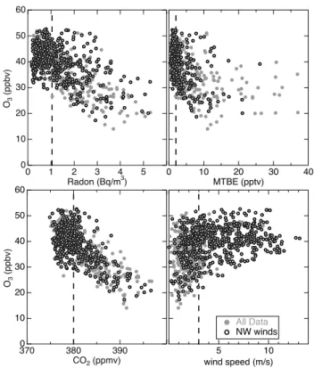
Fig. 2. Dependence of O3 upon parameters that indicate North
American continental influence. Data were collected 17 April– 23 May 2002 at Trinidad Head during the ITCT 2K2 field study (Goldstein et al., 2004; Millet et al., 2004). Open circles indi-cate one hour-average data collected during northwesterly winds (225◦≤wind direction≤360◦), gray circles indicate other wind di-rections. The vertical dashed lines indicate the independent variable values selected to separate marine data from those affected by con-tinental influences.
continental influences. Radon is emitted from continental but not oceanic surfaces, and with a radioactive decay half-life of 3.8 days, provides an excellent tracer of recent conti-nental contact of an air mass. Methyl-t-butyl ether (MTBE) (Schade et al., 2002) accounted for 11 to 15% by volume of the reformulated gasoline in California before its phase out at the end of 2002. With a lifetime of about 4 days at global mean OH concentrations MTBE also provided an ex-cellent tracer of recent continental impact during ITCT 2K2. In 2002 MTBE was quite specific to North American influ-ence, since at this time its input to the atmosphere was dom-inated by US production and use. Further, due to its high water solubility, MTBE is readily taken up by water surfaces and is thus expected to be strongly depleted in the MBL. Car-bon dioxide (CO2) has sinks (photosynthesis by vegetation)
and sources (respiration by vegetation and combustion) that are much stronger in the continental compared to the ma-rine environment. Figure 2 illustrates the correlation of O3
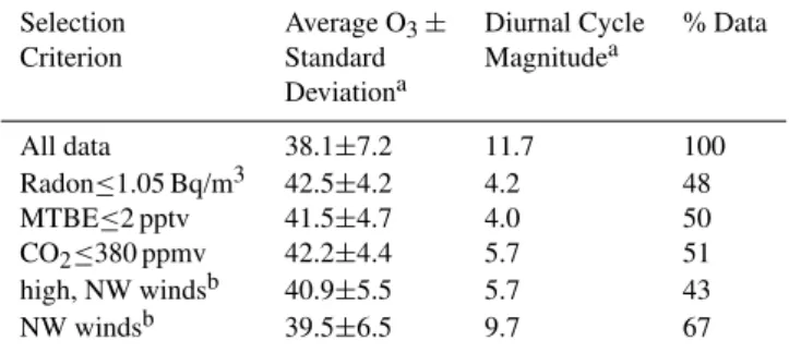
Table 2. Average O3 mixing ratios measured 17 April–23 May
2002 at Trinidad Head during the ITCT 2K2 field study (Goldstein et al., 2004; Millet et al., 2004) under different conditions. All re-sults derived from one-hour average measurements.
Selection Average O3± Diurnal Cycle % Data
Criterion Standard Magnitudea Deviationa
All data 38.1±7.2 11.7 100 Radon≤1.05 Bq/m3 42.5±4.2 4.2 48 MTBE≤2 pptv 41.5±4.7 4.0 50 CO2≤380 ppmv 42.2±4.4 5.7 51
high, NW windsb 40.9±5.5 5.7 43 NW windsb 39.5±6.5 9.7 67
aUnits of ppbv O
3; Peak-to-peak amplitude of diurnal cycle. bNW Winds: 225◦≤wind direction≤360◦;
high winds: wind speed≥3 m/s.
and MTBE (i.e. greater continental influence) correlate with lower O3mixing ratios, indicating that, at least in spring at
Trinidad Head, the primary continental influence on O3 is
surface deposition and/or destruction by reaction with local emissions. In continentally-influenced air reaching Trinidad Head in spring, evidently respiration by vegetation and pos-sibly emission by combustion processes dominate the CO2
budget, so that higher mixing ratios of CO2 also correlate
with lower O3mixing ratios.
Inspection of Fig. 2 allows the definition of mixing ratio thresholds of the three tracers that indicate continentally in-fluenced air at that location and time. These mixing ratios are taken to be the upper limits where the measured O3
be-gins to decrease noticeably. They are indicated by the ver-tical dashed lines in Fig. 2, and are listed in Table 2. The MTBE and CO2limits are the same as those utilized by Jaffe
et al. (2003) and Parrish et al. (2004a).
The tracer mixing ratio limits for selection of marine con-ditions provide a mechanism to assess the net effect of conti-nental impacts on the marine O3in the Trinidad Head ITCT
2K2 data set. The measured O3 at tracer mixing ratios less
than these limits are taken as characteristic of marine air. Ta-ble 2 lists the average and standard deviations of the ma-rine O3 mixing ratios evaluated by the three criteria. The
average results of the three tracer criteria indicate that dur-ing the sprdur-ing 2002 period of the ITCT 2K2 study, marine O3averaged 42.0 ppbv with a standard deviation of 4.4 ppbv.
The three derived averages and standard deviations all agree within≈1% and 7%, respectively. Notably, each tracer in-dicates that during about 50% of the time continental influ-ences significantly affected the measured O3 mixing ratios
during the ITCT 2K2 study period.
3.2 Selection of marine air by wind direction and speed Here we compare wind and chemical data as criteria for ma-rine air selection at Trinidad Head during the ITCT 2K2 study to inform our later interpretation of data from sites with wind data but no chemical measurements. It is rare to have extensive trace gas data sets available, but many O3
measurement sites collect simultaneous wind data. Figure 2 shows the O3 dependence on wind speed and direction in
the Trinidad Head ITCT 2K2 data set, and Fig. 3a shows this dependence in a wind rose format for spring 2007. It is clear that the continental effects (relatively low O3mixing
ratios) are predominately seen at low wind speeds and in sec-tors other than the prevailing northwesterly wind direction. Two features are notable. First, the continental effects, as in-dicated by systematically lower average O3, are seen at all
wind speeds, but their impact does decrease at higher wind speeds. Second, simply selecting northwesterly wind direc-tions without a wind speed criterion (open circles in Fig. 2) is not effective for isolating marine air. Depleted O3, as well
as enhanced mixing ratios of the three continental tracers, are seen in northwesterly winds, particularly at the lower wind speeds. Evidently transport, associated with mesoscale meteorological patterns such as land-sea breeze circulation and various orographic effects, can bring continentally influ-enced air ashore from the northwest wind sector. Table 2 indicates the resulting average O3 mixing ratios for
north-westerly winds, both with and without a wind speed selection criterion. During the ITCT 2K2 study period northwesterly winds occurred about two-thirds of the time, with an aver-age O3 mixing ratio of 39.5 ppbv and a standard deviation
of 6.5 ppbv, i.e. 6% smaller and 15% more variable than the average marine O3mixing ratio derived from the three trace
gas criteria. Adding the high-wind criterion (wind speeds ≥3 m/s) decreased the selected data to 43% of the total, but significantly improved the agreement of the derived average O3mixing ratio with the marine average: 40.9±5.5 ppbv
ver-sus 42.0±4.4 ppbv. In the following analyses, we will utilize simultaneous wind speed and direction data to approximately isolate marine air by selecting only those periods with rela-tively high, onshore winds.
Coastal orography affects the wind field along the North American coast (e.g. Burk et al., 1999), which, in turn, af-fects the O3 concentrations observed at coastal sites. This
orography-wind-O3 interaction makes the determination of
the marine O3easier in some ways and more difficult in
(a)
(b)
Fig. 3.Wind rose for all one hour-average wind data collected during(a)spring 2007 at Trinidad Head and(b)spring 2003 at Olympic NP. Note the factor of 2 expanded wind speed scale in (b). The symbols are color-coded according to the measured O3mixing ratios plotted in
order of decreasing O3so that the lower O3mixing ratios are more clearly visible. To the left of the heavy dashed lines indicates the marine data sector defined here: high (wind speed≥3 m/s at Trinidad Head and≥2 m/s at Olympic NP), northwesterly winds (225◦≤wind direction
≤360◦).
the coast can be directly compared. However, turbulent flow driven by variations in the coastal orography may mix con-tinentally affected air from more northerly coastal locations into the air mass as it moves down the coast. Thus, even under onshore flow conditions with no apparent effects from the land-sea breeze circulation, some continental effects on the observed O3 can be present. However, the good
agree-ment of the wind-selected O3 averages (including the high
wind speed criterion) with the trace species-selected O3
av-erages indicates that the high, northwest wind filter is an ef-fective tool for isolating the marine O3 signature. It should
be noted that these orographic effects cannot be resolved by large-scale meteorological data, and trajectories based on these data (e.g. Oltmans et al., 2008). Such trajectories do provide information on the large-scale flow that brings ma-rine air masses to the North American coast, but they are unreliable for selecting against continental effects within the MBL.
A comparison of the derived marine mixing ratios of CO2
in Table 3 with the mixing ratios obtained from NOAA GMD flask data provides a further check of the effective-ness of the wind criteria for the selection of marine data. At Trinidad Head the wind-selected marine air gave an av-erage of 379.4±2.9 ppmv, and the monthly averages derived from the flask data are 378.35 and 378.91 ppmv for April and May 2002, respectively. These flasks are filled to best
repre-Table 3.Average mixing ratios±standard deviations measured 17 April–23 May 2002 at Trinidad Head during the ITCT 2K2 field study (Goldstein et al., 2004; Millet et al., 2004) compared for all data and different criteria for selection of marine conditions. All results derived from one-hour average measurements.
Species All data High, % ≤Selection %
NW Windsa Data Criteriab Data Radon (Bq/m3) 1.4±1.1 1.2±1.0 45 0.6±0.2 48 MTBE (pptv) 4.4±5.6 2.0±2.2 45 1.3±0.4 50 CO2(ppmv) 381.2±4.5 379.4±2.9 47 378.0±4.5 51
O3(ppbv) 38.1±7.2 40.9±5.5 43 – –
aNW Winds: 225◦≤wind direction≤360◦;
high winds: wind speed≥3 m/s
bSelection Criteria given in Table 2 and discussed in text
sent onshore flow of marine air. The average of the wind-selected marine data are consistent with a small positive bias compared to the flask data, reflecting some continental in-fluence even under high, on-shore wind conditions. This is also consistent with the chemical tracers; the wind selection gives slightly lower O3 than the MTBE or radon selection
60
50
40
30
20
10
0 O3
(ppbv)
00:00 06:00 12:00 18:00 00:00
time of day
Radon ≤ 1.05 Bq/m3 MTBE ≤ 2 pptv CO2≤ 380 ppmv high, NW winds
NW winds
All Data
Fig. 4. Diurnal cycle of O3for 17 April–23 May 2002
measure-ments at Trinidad Head during the ITCT 2K2 field study (Gold-stein et al., 2004; Millet et al., 2004). Gray closed circles in-dicate all one hour-average data, and black open circles inin-dicate those data collected during high (wind speed≥3 m/s), northwest-erly winds (225◦≤wind direction≤360◦). The color-coded, larger open symbols connected with lines indicate two hour-averages of data selected by the criteria annotated.
3.3 Diurnal cycle of ozone mixing ratio – a diagnostic of marine air selection
Here we examine the diurnal cycle of O3mixing ratio in the
MBL as a diagnostic for the success of our marine air se-lection criteria. Later (Sect. 5.2) we examine the O3diurnal
cycle in the context of the chemical environment of the MBL. A large amplitude diurnal O3cycle is generally observed at
continental surface sites (e.g. Trainer et al., 1987) due to the interaction of the pronounced diurnal evolution of the conti-nental boundary layer depth coupled with the conticonti-nental in-fluences on O3discussed previously. During nighttime, the
continental boundary layer is generally quite shallow, and O3
is markedly reduced by deposition and reaction with species emitted at the surface. In the vicinity of significant anthro-pogenic NOx sources and in locations with particularly stable nocturnal boundary layers, nighttime O3 mixing ratios can
approach zero. As the depth of the boundary layer grows fol-lowing sunrise, higher concentrations of O3are mixed down
from layers aloft that were isolated from the boundary layer removal processes during the nighttime. This mixing, com-bined with the influence of daytime photochemical produc-tion of O3, leads to the well-documented afternoon O3
maxi-mum, not only at highly polluted urban sites, but also at much less impacted rural sites.
The O3 diurnal cycle in the MBL is generally much
smaller than at continental sites, because the surface deposi-tion and titradeposi-tion loss processes are largely absent, and there is little diurnal evolution of the MBL. In the marine envi-ronment remote from emission sources, a small maximum at sunrise is followed by a small minimum near sunset (e.g. see Barbados and Samoa data in Oltmans and Levy, 1994). The afternoon minimum is attributed to daytime net photochem-ical destruction of O3in the low NOx, relatively moist and
warm environment of the MBL. The net photochemical de-struction is balanced by a downward flux of O3from the
rel-atively O3-rich free troposphere aloft. This downward flux is
approximately constant over the diurnal period, which leads to the sunrise O3 maximum following the nighttime hiatus
in the photochemical destruction. In the MBL downwind of continental sources, the NOx concentrations may be high enough to support net photochemical production of O3. For
example, Parrish et al. (1998) showed that a small afternoon O3maximum was seen at Sable Island, in closer proximity
to the North American NOx sources, while an afternoon O3
minimum was observed at a more remote MBL site on the Azores in the central North Atlantic. Importantly, reported O3diurnal cycles in the MBL are small (generally<
approx-imately 4 ppbv peak-to-peak). Thus, on the North American west coast, we will take the observation of a relatively strong diurnal cycle, especially with an afternoon maximum, as an indication of significant continental influence upon the mea-sured O3.
The expected differences in the diurnal cycle of O3in the
MBL and at continental sites provide a diagnostic of the suc-cess of our criteria for selecting marine air. Diurnal cycles in O3 at the Trinidad Head site calculated for six different
criteria are shown in Fig. 4, and the peak-to-peak ampli-tude of these cycles are given in Table 2. When all data are included, a relatively large amplitude cycle (≈12 ppbv) is apparent. This cycle is largely attributable to the land-sea breeze circulation. During the night and early morning off-shore winds bring O3-depleted air to the site from the
et al. (2008) with an amplitude≈10 ppbv, which is nearly as large as that derived from the full data set.
3.4 Comparison of Pacific coast marine boundary layer sites
To derive decadal trends in average O3from measurements
made for different time periods at different sites, it is impor-tant to quantify possible biases between the sites. At least two issues are of concern: first, since the sites to be consid-ered in the temporal trend determinations span 10◦of lati-tude (approximately 1000 km), there may be a spatial gradi-ent in average MBL O3that could bias the results, and
sec-ond, the dependence of measured O3on wind speed and
di-rection may vary between sites. In this section we apply the high speed, northwest wind data selection criteria discussed in Sect. 3.2 to the complete data sets at all four MBL sites with available wind data. As we will show, selection of data by the wind criteria does indeed provide measurements of the average MBL O3that are comparable across all four sites.
At the four sites with simultaneous wind and O3
measure-ments, the dependence of the measured O3on wind speed is
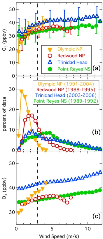
similar, but with some notable differences, particularly at low wind speeds. Fig. 5a shows the average O3measured as a
function of wind speed for northwesterly winds (225◦≤wind direction≤360◦) at four sites for all available springtime data. The years of the available data are given in Fig. 5b. As ex-pected from the discussion of Fig. 2, O3decreases at lower
wind speeds at each site due to the increasing effect of con-tinental influence at low wind speeds. This decrease is rea-sonably similar at three sites, but is significantly greater (i.e. lower measured O3at lower wind speeds) at Olympic NP,
than at the other three sites.
The distribution of measured wind speeds varies markedly between sites. The wind roses in Fig. 3 and the plot in Fig. 5b show that much lower wind speeds occur at Redwood NP and especially Olympic NP than at Trinidad Head and Point Reyes NS. The different wind speed distributions are at-tributed to differences in the local environments in which the sites and their wind sensors were placed. The two sites with relatively high wind speeds are well exposed to the large-scale wind flow. The Trinidad Head site is located below the summit of a promontory that extends out from the coastline, and Point Reyes is located in an unencumbered flat area of the Pt. Reyes Peninsula. In contrast the Redwood NP site is located on the side of a ridge with surrounding trees, and the Olympic NP site is located away from the west coast on the shore of the Juan de Fuca Strait within the city of Port Ange-les, Washington, providing more protected wind exposures at these two sites.
The average O3 dependence on wind threshold (Fig. 5c)
varies slowly for the Trinidad Head and Point Reyes NP data sets, the two sites with the best wind exposure. The Red-wood NP data set, collected at a more sheltered location, shows only a modestly stronger dependence on wind speed.
50
40
30
20
10
0
O3
(ppbv)
Olympic NP
Redwood NP Trinidad Head
Point Reyes NS
50
40
30
O3
(ppbv)
10 5
0
Wind Speed (m/s)
(a)
30
20
10
0
percent of data
Olympic NP (1991-2004)
Redwood NP (1988-1995) Trinidad Head (2003-2006)
Point Reyes NS (1989-1992)
(b)
(c)
Fig. 5.Springtime O3dependence on wind speed at four MBL sites.
(a)Symbols give average O3for 0.5 m/s wind speed increments;
some representative standard deviations of the averages are shown.
(b)Percent of data falling in 0.5 m/s wind speed increments. (c)
Average O3at all wind speeds higher than the indicated wind speed.
-10 -5 0 5 10
O3
difference (ppbv)
Pt. Reyes NS - Redwood NP
1.2 ± 2.2 r2 = 0.76 n = 16
Olympic NP - Redwood NP
0.4 ± 3.5 r2 = 0.34 n = 12
Olympic NP - Trinidad Head -1.2 ± 4.4
r2 = 0.29 n = 7
Olympic NP - Pt. Reyes NS
-0.3 ± 0.6 r2 = 0.99
n = 3
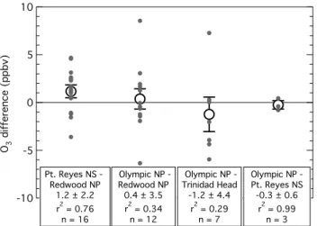
Fig. 6. Differences between simultaneous determinations of aver-age marine O3mixing ratios at four pairs of sites. Each small grey
symbol indicates the difference for one season in one year. Each large open symbol gives the mean difference for the pair of sites with the error bars indicating the one-sigma confidence limit of that mean. The annotations give the sites in each pair, mean differences
±standard deviations, square of the correlation coefficients for the individual seasonal average O3mixing ratios that led to the differ-ences, and the number of difference determinations.
(At the upper end of the observed wind speeds, the depen-dence of O3concentration becomes more variable due to
de-creasing frequency of higher wind speeds.) Compared to the other three sites, at Olympic NP, with a much more protected wind exposure (Fig. 5b), the average O3depends much more
strongly on wind threshold (Fig. 5c). This stronger depen-dence is attributed to a much stronger continental influence arising from the location of the site within Port Angeles, a city with a population of 20 000 and the major highway in the region. At low wind speeds, reaction of O3with local
an-thropogenic NO emissions is particularly effective in reduc-ing O3. Clearly the Olympic NP site is much more impacted
than the other three sites, and its suitability for characterizing marine mixing ratios of O3requires further discussion below.
Using wind data to select time periods to characterize ma-rine O3requires a balance between two competing concerns:
the desire to retain as much data as possible to achieve a sta-tistically precise measure of the average O3mixing ratio, and
the need to eliminate as fully as possible the continental influ-ences. Jaffe et al. (2003) selected 3 m/s (indicated by the ver-tical dashed lines in Fig. 5) as the best compromise of these two competing concerns. This same selection will be used here with the exception of the Olympic NP site. For this latter site a wind speed threshold of 2 m/s is selected since winds above this speed are relatively infrequent (Fig. 5b). It should be noted that the relationships shown in Fig. 5 are similar in other seasons, except that higher wind speeds are less fre-quent in autumn and winter, compared to spring and summer. Table 4 summarizes the percent of time that winds satisfy the
Table 4. Percentage of time during each season that data satisfy high, NW wind selection criteriaafor full data sets. All results de-rived from one-hour average measurements.
Site Winter Spring Summer Autumn Olympic N.P. 2.4 6.7 7.5 3.4 Redwood N.P. 3.3 13 10 5.8 Trinidad Head 13 30 29 20 Point Arenab – 61 – – Point Reyes N.S. 24 49 55 34
a225◦≤wind direction≤360◦; wind speed≥3 m/s, except≥2 m/s
at Olympic N.P.
bdata from 14 days in 1985
selection criteria in each season at each site. Such periods vary from quite infrequent (only 2 to 6% of the time in au-tumn and winter at the two more protected sites) to nearly one-third of the time in spring and summer at Trinidad Head and about one-half of the time in those two seasons at Pont Reyes NS.
Since the Olympic NP data site has the longest, continu-ous data set (over 23 years) in the MBL at the west coast of North America, it is important to include those data in the analysis. However, its location away from the west coast it-self and the relatively few data that can be considered due to its protected location raise concerns regarding the repre-sentativeness of that data set. Although this site location is far from optimal, Fig. 3b shows that the high winds occur from the west-northwest, which is the orientation of the Juan de Fuca Strait. Hence, the O3mixing ratios selected by the
wind criteria do represent direct Pacific airflow through the Juan de Fuca Strait to the site. Such flow does occur only a small fraction of the time. For example, during spring 2003 (the data included in Fig. 3b) only 72 h of O3data meet the
wind selection criteria. This corresponds to 3.2% of the total hours in that 3-month period and 3.6% of the measurement time covered by the available data. However, the diurnal land-sea breeze cycle plays a significant role in determining wind speeds with the high, northwest winds occurring pre-dominately for a few hours in the afternoon on many days. Those 72 h of selected data represent 17 different days in all three months of the season. While it would be desirable to have measurements available from all days, the 17 days with suitable data nevertheless provide a reasonably representa-tive sample of days, a sample that compares favorably with the once per week schedule often employed by the few in-tensive sites conducting O3sonde launches. These
consider-ations indicate that the Olympic NP data set does provide a valuable characterization of MBL O3.
It is notable in Fig. 5a and 5c that the O3 measured at
while the result from these latter two sites agree well. As will be discussed further below, this difference is primarily due to the different measurement periods at these sites. The Trinidad Head data were collected more than a decade later than the other two data sets, and the decadal trend in marine O3, which is a primary focus of this paper, accounts for this
difference.
Comparison of the seasonal average O3mixing ratio
mea-sured at two different sites in the same year provides a means to check for (1) biases between sites, and (2) the confidence limit that can be assigned to the seasonal average O3at either
site. There is only relatively limited overlap in the measure-ment time periods between the sites considered here. Fig-ure 6 shows the differences in the seasonal average marine O3simultaneously determined at the four pairs of sites that
have simultaneous measurements. The average bias between the sites in each of the four pairs is 1.2 ppbv or less. Only one average bias is statistically significant at the one-sigma con-fidence level, and none are significant at the two-sigma level. Hence, there is no evidence for a statistically significant bias over the four sites represented in these pairs, which cover the full latitude range of the sites to be used in the next section to derive decadal trends. The scatter of the ratio determi-nations in Fig. 6 provides a means to estimate confidence limits for the annual, seasonally averaged MBL O3 mixing
ratio measured at each site. The standard deviation of the 38 differences included in the Fig. 6 is 3.1 ppbv. Propaga-tion of error procedures (see, e.g. Bevington, 1969) indicate that the variance (i.e. square of the standard deviation) of a difference between two numbers is equal to the sum of the variance of the two numbers. As a rough guide to assessing statistical fits, we assume that the confidence limits of the O3
averages at all four sites are approximately equal. This im-plies that the 1σ confidence limit for a seasonal average O3
determination in each year is approximately 2.2 ppbv. In the following section, this confidence limit will be used to evalu-ate the goodness of the statistical fits in the determination of decadal trends.
4 Decadal trends
Our goal here is to determine long-term O3 trends in the
MBL at the west coasts of North America and Europe, and to investigate the seasonal variation in these trends. For Europe, we utilize the monthly mean O3data from Mace Head,
Ire-land (Table 1 of Derwent et al., 2007) that were selected as baseline air; three-month seasonal averages are simply cal-culated from those numbers. For North America, we will examine trends from two separate data sets - the trend from Olympic NP and one composite trend from four sites with shorter records: Redwood NP, Trinidad Head, Point Arena, and Point Reyes NS. Data from these sites will be selected for marine air by means of a high (wind speed≥3 m/s, ex-cept ≥2 m/s at Olympic N.P.), northwesterly (225◦≤wind
direction≤360◦) wind window, which Sect. 3 shows is rea-sonably effective. As discussed below the trends derived from the two separate data sets are consistent, and one, more accurate and precise trend is derived by combining measure-ments from all five sites into one composite data set. 4.1 Statistical approach to trends analysis
The ability to discern temporal trends in MBL O3from the
relatively short, decadal time scale data records that are avail-able is limited by two factors: first, our ability to accurately and precisely determine the average O3mixing ration in each
year, and second, the interannual variability in the average O3
between years that systematically differs from the assumed functional form of the temporal trend. To minimize these limitations we improve the precision of the yearly average O3mixing ratio determination through three strategies. First,
elimination of continental influences to the fullest extent pos-sible substantially reduces the variability in the measured O3
(see Figs. 2 and 4). Second, seasonal rather than monthly or shorter period averaging takes advantage of the reduced variability brought by longer-term averages. It should be noted that averaging over seasons and considering the tem-poral trend in each season separately avoids the “deseason-alization” process employed in some work (e.g. Harris et al., 2001; Jaffe and Ray, 2007), which introduces unneeded com-plexity and potentially can confound the trend analysis if dif-ferent seasons exhibit difdif-ferent temporal trends. Finally, in-clusion of as much data as possible improves the precision to which the annual average O3can be determined. Thus, the
combination of the data from the five North American MBL sites with available wind and O3data provides the most
pre-cise determination of temporal trends for that continent. We primarily rely upon the simplest possible functional form for trend determination. For each season, a linear-least squares fit is made to a two-parameter equation:
[O3]=slope∗(year−2000)+intercept (1)
This slope, in units of ppbv/yr, provides the average yearly increase in O3mixing ratio over the period of the data record,
and the intercept provides the interpolated, seasonally aver-aged O3 mixing ratio in the year 2000. It should be noted
that the utilization of a linear fit does not imply that the tem-poral trend is necessarily linear, and does not imply that the trend was linear before the data period or will continue lin-early into the future. 95% confidence limits are assigned to each parameter as a test of significance. Further, the statistic
χν, which we define here as the square root of reduced chi-square (Bevingtion, 1969), is given. If Eq. (1) adequately fits the data to within ability of the data to determine the av-erage O3in each year (i.e. the first factor discussed in the
preceding paragraph) thenχνapproximately equals the con-fidence limit on the determination of the annual seasonal av-erage O3 mixing ratio. As discussed in the preceding
50
40
30
20
O3
(ppbv)
2010 2000 1990 1980
Summer
2010 2000 1990 1980
Autumn 50
40
30
20
O3
(ppbv)
Winter
Olympic NP Redwood NP Trinidad Head Pt. Arena Point Reyes NS Mace Head Spring
Fig. 7. Comparison of trends in MBL O3at the Pacific Coast of
North America and at Mace Head, Ireland. Each data point is a seasonal three month average in a given year at the site specified by color and symbol. Linear least-squares fits are given for all Pacific sites (black lines), the Olympic NP data (orange lines), the Pacific sites excluding the Olympic NP data (gray dotted lines), and Mace Head (purple solid lines). Olympic NP data are not available for summer. Second degree polynomial fits (Eq. 2) to the Mace Head data are indicated by the purple dotted lines.
North American data sets. Ifχν is significantly larger than the confidence limit, then significant interannual variability or a temporal trend systematically different from the linear dependence in Eq. (1) is expected. In the latter case, the statistical significance of a third parameter, acceleration, is tested:
[O3]= slope2000
∗
(year−2000)+intercept
+0.5∗acceleration∗(year−2000)2 (2) Here acceleration, in units of ppbv/yr2, represents the av-erage rate of increase of d[O3]/dt over the period of the data
record and slope2000is the value of d[O3]/dt in the year 2000.
In Eq. (2) the slope2000is the rate of increase of O3in the year
2000, and the rate of increase changes with time rather than representing the average yearly increase in O3, as was the
case in Eq. (1). The factor of 0.5 is required in the last term of Eq. (2) so that the acceleration has the defined meaning, as can be verified by differentiating Eq. (2).
(a)
(b)
Fig. 8. Temporal trends derived for spring(a)at Olympic NP and
(b)for the other MBL sites as a function of wind selection. The Olympic NP Visitors Center data are the same as discussed else-where in the paper. The Port Angeles data were collected by the park staff at a nearby site before the National Park service moni-toring program was established. In (a) linear least-squares fits are given for both data sets (blue lines) and for the Visitor Center data only (orange lines). The slopes of the former fits are given in the figure annotations. In (b) the wind selected data from Fig. 7 are shown in lighter colors, while the data for all winds are in darker colors.
4.2 Sea level, marine boundary layer temporal trends Significant increases in MBL O3are found in all west coast
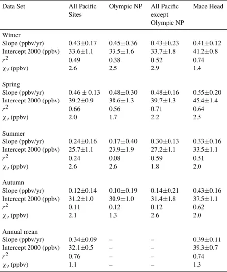
Table 5.Linear Regression results for decadal trends in MBL O3mixing ratios derived from different data sets and different seasons. The
95% confidence limits are given for the slopes and intercepts.
Data Set All Pacific Olympic NP All Pacific Mace Head Sites except
Olympic NP Winter
Slope (ppbv/yr) 0.43±0.17 0.45±0.36 0.43±0.23 0.41±0.12 Intercept 2000 (ppbv) 33.6±1.1 33.5±1.6 33.7±1.8 41.2±0.8
r2 0.49 0.38 0.52 0.74
χν(ppbv) 2.6 2.5 2.9 1.4
Spring
Slope (ppbv/yr) 0.46±0.13 0.48±0.30 0.48±0.16 0.55±0.20 Intercept 2000 (ppbv) 39.2±0.9 38.6±1.3 39.7±1.3 45.4±1.4
r2 0.66 0.56 0.71 0.64
χν(ppbv) 2.0 1.7 2.2 2.5
Summer
Slope (ppbv/yr) 0.24±0.16 0.17±0.40 0.30±0.13 0.33±0.16 Intercept 2000 (ppbv) 25.7±1.1 23.9±1.9 27.2±1.1 33.5±1.1
r2 0.24 0.08 0.59 0.51
χν(ppbv) 2.6 2.6 1.8 2.0
Autumn
Slope (ppbv/yr) 0.12±0.14 0.10±0.19 0.14±0.21 0.43±0.16 Intercept 2000 (ppbv) 31.2±1.0 30.9±1.0 31.4±1.8 37.5±1.1
r2 0.11 0.12 0.12 0.62
χν(ppbv) 2.1 1.3 2.6 2.0
Annual mean
Slope (ppbv/yr) 0.34±0.09 – – 0.39±0.11 Intercept 2000 (ppbv) 32.1±0.5 – – 39.3±0.7
r2 0.76 – – 0.74
χν(ppbv) 1.1 – – 1.3
quite remarkable in some seasons. For example in spring the average temporal trends (i.e. slopes) for Olympic NP and for the combined data set are significantly larger than zero at the 3σ and 6σ levels, respectively. These trends are derived from completely independent data sets. Thus, the trend de-rived by combining all Pacific sites is the best determination of the North American trend, and in spring it is significantly larger than zero at the 7σ level. The springtime increase in MBL O3over the 1985 to 2007 period, which was first
re-ported by Jaffe et al. (2003), is statistically significant to a degree that is essentially beyond question.
The results for Olympic NP are considerably less certain than those from the combined data set. This greater uncer-tainty arises from the small fraction of data meeting the wind selection criteria (2 to 8% of the time, depending on season), and the greater impact of local emissions due to the location of the measurement site within the Port Angeles city area and its proximity to the major regional highway in that city. In summer, the season of the large majority (nearly 75%) of
tourist visits to Olympic NP, the local effects influence ob-served O3to such an extent that summer data from this site
are not included in Fig. 7, although the summer linear regres-sion results are given in Table 5 and these data are included in the calculation of 12 month running means in Sect. 6. In each season, the year 2000 intercept of the linear fit to the Olympic NP data is slightly lower than that obtained from the combined data set, although this difference is not statisti-cally significant except in summer.
are notable in Fig. 8. First, the derived slopes of linear fits to the data are not strong functions of the selected wind crite-ria, and the results in Fig. 8 are in statistical agreement with those listed in Table 5. Second, in contrast to the slopes, the year 2000 intercepts are a strong function of the wind selec-tion. The high, northwest wind selection greatly reduces the effects of the local influences, which act to reduce the mea-sured O3, and is particularly important for determining the
absolute O3mixing ratios in the marine air. Third, the
ear-lier data (blue squares in Fig. 8a), while not subjected to the same quality control measures as the later data, do suggest that the increasing trend in MBL O3began before 1985, the
date of the earliest data included in Fig. 7. In summary, the results in Fig. 8 indicate that the wind selection criteria do not strongly influence the derived temporal trends, although they are important for comparing absolute O3mixing ratios
measured at sites with different local influences.
Despite the comparison shown in Fig. 6 and the associ-ated discussion, which establishes that the data collected at the four separate sites can be directly compared, it would be preferable if a long-term record of O3had been collected
at a single site, so that combining data from separate sites would not be necessary. One way to approach this more ideal situation would be to reestablish measurements at the Redwood NP and Point Reyes NS sites, which were termi-nated in 1995 and 1992, respectively. Measurements for only a few additional years would quickly establish whether the present O3 mixing ratios have exceeded those measured in
the early 1990s by the amount suggested by the trends de-rived in Fig. 7. One quick test of this approach is a direct comparison of the seasonal averages measured at Trinidad Head from 2002–2007 with those measured at Redwood NP from 1988 to 1995. These sites are both on the California coast within 35 km of each other. It is straightforward to calculate an average O3 mixing ratio with confidence limit
for all of the data measured in each season at each site that satisfy the wind selection criteria. The differences in these averages divided by the number of years between the cen-tral time of each data set (13 or 13.5 years) gives an approx-imate trend, and error propagation techniques provide 2σ
confidence limits for those trends. The results are highly sta-tistically significant for all seasons, and agree well with the trends listed in Table 5: 0.46±0.29, 0.47±0.18, 0.34±0.18, and 0.25±0.15 ppbv/yr in winter, spring, summer and au-tumn, respectively. Of course this agreement is expected, since these data are all included in the composite linear re-gression. In summary, all of the data sets examined, both by linear regression techniques and this simpler analysis, indi-cate that statistically robust increases have occurred in the O3
mixing ratio in the MBL adjacent to the west coast of North America.
4.3 Data available from other sites
Of the nine sites listed in Table 1, data from only five were included in the trends discussion in Sect. 4.2. Data sets from the other four were excluded for several reasons. For com-pleteness, those reasons are briefly discussed here.
Jaffe et al. (2003) included the Cheeka Peak data in some of the linear fits that they discussed. The O3measured at this
site generally lay above the trends from the other, near sea level sites. This difference is expected because Cheeka Peak is located on a relatively isolated peak at an elevation near 0.5 km. The O3in the MBL along the North American west
coast has a strong vertical gradient (e.g. see Fig. 15 of Olt-mans et al., 2008) so that the Cheeka Peak measurements are expected to be several ppbv higher than the sea level mixing ratios. Thus, the Cheeka Peak data cannot be combined with the sea level data sets, and are not discussed further in this paper.
The earliest available data were collected at Quillayute, Washington in 1974–1975 (Singh et al., 1978). If these data were reliable it would be desirable to include them in the trend analysis to extend the time period covered by available data. However, these measurements were made by a chemi-luminescence technique, and no information is available re-garding calibration and quality control procedures. The US EPA suggests not including data collected before standard-ized procedures were implemented in 1979 or 1980. Further, no wind data or other measurements are available to elimi-nate continental effects from the data set. Singh et al. (1978) suggest that these data may have been influenced by transport from Portland, Oregon or from the Seattle-Tacoma, Wash-ington area. Therefore these data are not considered further here.
The California Air Resources Board has made O3
mea-surements at Yreka, California since 1981. Oltmans et al. (2006, 2008) have used these data to suggest that there likely has not been a significant impact of changing back-ground O3amounts reaching the US west coast. This
sug-gestion clearly conflicts with the conclusions reached in the preceding section, but unfortunately the Yreka site is ex-tremely poorly situated from both regional and local per-spectives rendering it unsuitable for characterizing marine O3levels. Regionally, it is located approximately 125 km
in-land in the Klamath River Valley behind the Klamath Moun-tains, a particularly high section of the North American west coastal ranges. Therefore, the Yreka site always sits within the continental boundary layer, and never directly receives marine air inflow. Marine air is certainly entrained into the continental boundary layer, and trends in the O3 measured
at Yreka could still possibly reflect trends in the marine O3
moving inland from the Pacific Ocean. However, the local environment of the site precludes a simple investigation of background O3trends (see map in Fig. 9). Yreka is well
Yreka, California
Fig. 9. Monitoring site map (downloaded from CARB website http://www.arb.ca.gov/qaweb/site.php?s arb code=47861) and O3 trends analysis for the Yreka, California site indicated by the red circle on the map. The heavy orange line just west of the site indi-cates the I-5 interstate highway and the light grey line just east of the site indicates a rail line. The parameters of the linear least-squares fits (straight lines) are given in Table 6.
the US west coast. Further, the major US west coast north-south rail line also passes through the Klamath River Val-ley approximately 5 km to the east of the site. The emis-sions from these transportation sources certainly perturb the O3mixing ratios at Yreka, both through titration of O3by
fresh NO emissions and production of O3under
photochem-ically favorable conditions. Consideration of the temporal trends of these local perturbations is required when evaluat-ing trends in O3 at Yreka. For example, heavy-duty truck
traffic, the major source of on-road NOx emissions in the US, increased at an average rate of about 2%/yr between 1992 and 2005 (data available from http://www.dot.ca.gov/ hq/traffops/saferesr/trafdata/). An additional difficulty arises from several problems in the archived Yreka O3data set
it-self. First, for some periods, particularly near the start of the record, data were recorded with a precision of only 10 ppbv, and for others, particularly near the end of the record, data were recorded with a precision of 1 ppbv. This changing pre-cision may confound any trends analysis. Second, some data
Table 6.Linear Regression results for mid-day (12:00–18:00 LST) Yreka O3mixing ratio data set for different seasons. The 95%
con-fidence limits are given for the slopes and intercepts.
Season Winter Spring Summer Autumn
Slope (ppbv/yr) −0.11±0.33 0.09±0.26 0.30±0.33 0.31±0.32 Intercept 2000 (ppbv) 21.6±3.2 42.2±2.9 46.1±3.2 35.1±3.3
r2 0.03 0.03 0.15 0.15
χν(ppbv) 5.1 4.1 5.1 5.4
sets have measured zero O3 mixing ratios removed. These
missing data, particularly when combined with the changing instrument precision, also may confound the trends analysis. Finally, there are periods in the record that appear to indicate improper instrument performance. Oltmans et al. (2008) re-moved one such period (the year 2001), but several other, shorter periods of suspicious data are also present.
If we ignore the problems in the data archive, we can pro-ceed with a trend analysis for the measured O3at Yreka. No
meteorological data are available to preferentially select pe-riods favorable for elucidating the impact of marine O3, so
we will follow the strategy of Oltmans et al. (2008) of select-ing data from the later part of the daytime period (12:00– 18:00 LST). The results of the trend analysis is shown in Fig. 9 and summarized in Table 6. The trends in summer and autumn are positive and nearly significant at the 95% confi-dence level, which is in accord with the positive trends noted by Oltmans et al. (2008). However, the absolute O3mixing
ratios in summer at Yreka are nearly twice those measured at the MBL sites (compare intercept 2000 between Tables 5 and 6) The wintertime trend is negative in accord with the discussion of by Oltmans et al. (2008), but the trend derived here is not statistically significant. Notably, the absolute O3
mixing ratios in winter at Yreka are only about 60% of those measured at the MBL sites, and this difference is statisti-cally significant. These differences between the Yreka and the MBL data clearly indicate that the O3 mixing ratios at
Yreka have been strongly modified from the marine environ-ment. In summary, a careful analysis of the Yreka data set might be able to elucidate the behavior of O3 in the
heav-ily impacted transportation corridors in rural regions of the United States, but these data cannot provide any direct in-formation regarding trends in MBL O3 entering the North
American west coast. In particular, statements regarding the impact of changing background O3 mixing ratios reaching
the west coast (Oltmans et al., 2006, 2008) cannot be justi-fied on the basis of the Yreka data set.
The Channel Islands NP off the coast of Los Angeles in Southern California is another potentially attractive site for investigating marine O3. Oltmans et al. (2008) present
trajec-tory calculations and suggest that this site is able to provide information on background O3 entering the US. However,
50
40
30
20
O
3(ppbv)
00:00
06:00
12:00
18:00
00:00
time of day
Season
∆
O
3(ppbv)
Winter
3.2
Spring
4.0
Summer
5.0
Autumn
5.7
50
40
30
20
10
0
O
3(ppbv)
12
10
8
6
4
2
0
Month
Olympic NP
Redwood NP
Trinidad Head
Point Reyes NS
24
(a)
(b)
Fig. 10.Seasonal and diurnal cycles of MBL O3derived from the
data sets collected at the four sites indicated in the figure annota-tion. The decadal trends were removed from the data before deriv-ing these cycles by correctderiv-ing each year’s data to the reference year 2000 according to the temporal trends given in Table 5. The diur-nal cycles are averages of the cycles derived for Trinidad Head and Point Reyes NS.
is unable to resolve the complex circulation patterns that are prevalent along the North American west coast south of San Francisco. These complex patterns, which have spatial scales of 10 s of km, include the “Catalina Eddy” (Mass and Al-bright, 1989; Skamarock et al., 2002), and effectively circu-late heavily impacted continental air from the Los Angeles urban area into the vicinity of Channel Islands NP. Without detailed mesoscale meteorological modeling of the flow to this site, it will be difficult to glean information on
unper-turbed marine O3mixing ratios. Data from this site will not
be considered further here.
4.4 Nonlinearity of temporal trends
Derwent et al. (2007) have shown that at Mace Head the temporal trends have decreased to the point that the baseline O3mixing ratios have approximately stabilized in the years
since 2000. This behavior is evident in Fig. 7 and quantified by the fits to Eq. (2) that are included as dotted purple lines in those plots. In all seasons except autumn, the acceleration term is negative (−0.03 to−0.07 ppbv/yr/yr) with statistical significance at the 79 to 93% confidence level. In contrast, the MBL trends at the North American west coast show no statistically significant indication of non-linearity.
5 Systematic variations in marine boundary layer ozone
Besides the decadal scale temporal trends discussed in Sect. 4, there are seasonal and diurnal cycles as well as sys-tematic variations with synoptic scale flow conditions that are all relevant to our understanding of O3in the MBL. Our
goal in this section is to investigate those variations. To com-pare results from data sets collected over different time pe-riods from different sites, all of the data collected within the wind criteria for marine air selection were detrended by subtracting from each O3 measurement a term equal to
slope∗(year-2000), where the slope is taken from the first col-umn of Table 5. In effect, this adjusts the data to what would have been measured if all data had been collected in the year 2000.
5.1 Seasonal cycles
The seasonal cycles derived from the four MBL data sets that cover all seasons are shown in Fig. 10a. The seasonal cycles derived from all four data sets are in excellent agree-ment, although the summertime results from Olympic NP are somewhat lower due to the difficulty of eliminating local ef-fects at that site in that season. This close agreement again emphasizes the comparability of the measurements made at the different sites. The cycles in Fig. 10a are in good agree-ment with the seasonal cycles shown in Fig. 18 of Oltmans et al. (2008), although the present results are somewhat lower in magnitude than most of the years included there. This dif-ference arises because the present results represent the year 2000, while the Oltmans et al. (2008) cycles represent the different years 2002–2007.
5.2 Diurnal cycles
It is difficult to accurately determine the diurnal cycle of marine O3 from measurements made at a surface site on