www.geosci-model-dev.net/6/2087/2013/ doi:10.5194/gmd-6-2087-2013
© Author(s) 2013. CC Attribution 3.0 License.
Geoscientiic
Model Development
Correction of approximation errors with Random Forests applied to
modelling of cloud droplet formation
A. Lipponen1, V. Kolehmainen1, S. Romakkaniemi1, and H. Kokkola2
1Department of Applied Physics, University of Eastern Finland, P.O. Box 1627, 70211 Kuopio, Finland 2Finnish Meteorological Institute, Kuopio Unit, P.O. Box 1627, 70211 Kuopio, Finland
Correspondence to:A. Lipponen ([email protected])
Received: 1 March 2013 – Published in Geosci. Model Dev. Discuss.: 19 April 2013 Revised: 23 October 2013 – Accepted: 30 October 2013 – Published: 16 December 2013
Abstract.In atmospheric models, due to their computational time or resource limitations, physical processes have to be simulated using reduced (i.e. simplified) models. The use of a reduced model, however, induces errors to the simulation results. These errors are referred to as approximation errors. In this paper, we propose a novel approach to correct these approximation errors. We model the approximation error as an additive noise process in the simulation model and em-ploy the Random Forest (RF) regression algorithm for con-structing a computationally low cost predictor for the ap-proximation error. In this way, the overall simulation prob-lem is decomposed into two separate and computationally efficient simulation problems: solution of the reduced model and prediction of the approximation error realisation. The ap-proach is tested for handling approximation errors due to a reduced coarse sectional representation of aerosol size dis-tribution in a cloud droplet formation calculation as well as for compensating the uncertainty caused by the aerosol acti-vation parameterization itself. The results show a significant improvement in the accuracy of the simulation compared to the conventional simulation with a reduced model. The pro-posed approach is rather general and extension of it to dif-ferent parameterizations or reduced process models that are coupled to geoscientific models is a straightforward task. An-other major benefit of this method is that it can be applied to physical processes that are dependent on a large number of variables making them difficult to be parameterized by tradi-tional methods.
1 Introduction
In numerical simulations of complicated physical pheno-mena, one usually has to balance between the model accu-racy and the computation time. Reduction in computation time is typically obtained by using reduced models for some of the functions in the model. The use of reduced models, however, result in errors in model output. The errors are re-ferred to as the approximation errors (AE).
In this paper, we consider the approximation errors caused by coarse discretization of aerosol size distributions in sec-tional aerosol models. In secsec-tional models, the continuous aerosol particle size distributions are represented with dis-crete size sections (e.g. Weisenstein et al., 2007; Jacobson, 2001; Rodriguez and Dabdub, 2004; Kokkola et al., 2008). The accuracy of the description of the size distribution in-creases with increasing number of size sections. The compu-tational demand of the model, however, is heavily increased with the number of the sections. Therefore, a compromise between the model accuracy and the computational time has to be made to construct a feasible model for simulations of atmospheric scale.
2088 A. Lipponen et al.: Correction of approximation errors with RF
would reduce the uncertainty in the estimated aerosol indi-rect effect. Current aerosol-climate models include param-eterizations for calculating cloud activation of aerosol that use the above mentioned sectional approach (Abdul-Razzak and Ghan, 2002; Nenes and Seinfeld, 2003). These param-eterizations introduce uncertainty in CDNC estimation due to highly simplified description of aerosol activation process. Beyond this, coarse size resolution of the aerosol size distri-bution that is used as an input for a cloud activation parame-terization translate to approximation errors in the calculated aerosol indirect effect.
Recently, an approach for compensating approximation errors in inverse problems was proposed by Kaipio and Somersalo (Kaipio and Somersalo, 2005). The approach is known as the approximation error approach. This far, the approach has mainly been applied to so-called soft field to-mography imaging problems that are related to estimation of spatially distributed parameters of partial differential equa-tions from boundary measurements. In such problems, the approach has been successful, for example, in compensa-tion of approximacompensa-tion errors due to coarse finite element discretization (Arridge et al., 2006; Nissinen et al., 2009), unknown nuisance parameters (Nissinen et al., 2009, 2011; Kolehmainen et al., 2011), and the truncation of the compu-tational domain (Lehikoinen et al., 2007; Kolehmainen et al., 2009).
The main idea in the approximation error approach is to model the error between the accurate and approximate com-putational models as an additive noise process. The realisa-tion of the approximarealisa-tion error noise is obviously unknown and cannot be computed without solving the accurate model and knowing the unknown parameters. However, given the prior probability density models of all the unknowns, the inverse problem can be marginalized over the unknown ap-proximation error in an approximate way by utilising a Gaus-sian estimate for the joint probability density of the approxi-mation error and the unknown parameters. For a detailed ex-planation, see Kolehmainen et al. (2011).
In this paper, we propose a novel approach for handling approximation errors in simulation models. The approach is an extension of the approximation error approach. Similarly as in applications of the approximation error approach to in-verse problems, the discrepancy between the outputs of accu-rate and reduced models is modelled as an additive approx-imation error noise process in the simulation model. How-ever, whereas in the framework of inverse problems the un-certainty related to the approximation errors is taken care of by marginalization, here we propose to construct a computa-tionally low-cost predictor model that computes an estimate for the realisation of the approximation error given in the in-put parameters and solution of the reduced model. This way the solution of the simulation problem is decomposed into a computationally efficient approximation of solving the re-duced computation model and estimating the value of the ad-ditive approximation error.
One computationally simple and light-weight and recently widely used function approximation approach is to employ RFs. The RFs are predictive models introduced in Breiman (2001). A RF model consists of an ensemble of binary tree predictors. Each of these tree predictors is trained based on the training data.
The aim of the RF model construction is to get numer-ous tree models that slightly differ from each other. This is achieved by introducing randomization in the tree construc-tion. The constructed RF models are further used for the function output prediction. The prediction of the RF model is computed by averaging the predictions of each (almost) unbiased tree model in the ensemble. This averaging should therefore increase the accuracy of the RF model over a sin-gle tree prediction accuracy. Recently, the RF models have been applied to classification and regression problems in-cluding classification of climate zones (Bechtel and Daneke, 2012), earthquake induced damages (Tesfamariam and Liu, 2010), remote-sensing data (Pal, 2005) and disease predic-tion (Munro et al., 2006; Yao et al., 2013). In papers by Bechtel and Daneke (2012), Tesfamariam and Liu (2010), Pal (2005), a comparison between different algorithms were carried out. Despite its simplicity, the RF was observed to perform at least equally well as the more complicated algo-rithms in classification and regression problems.
We employ the RF approach for construction of the pre-dictor model for the approximation errors in the simulation model. Here it should be noted that the proposed approach is not restricted to the RFs only and some other type of models, such as neural networks (Rojas, 1996; Haykin, 2009), could have been used as well. The training data for the RF algo-rithm is a set of approximation error realisations between the accurate and reduced models corresponding to a set of random samples of the input parameters that are sampled from the prior probability density models. The computation of the training data involves solution of the computationally demanding accurate model as many times as the number of samples. This step, however, can be done as precomputa-tion and needs to be carried out only once. Given the trained RF model, the accurate model can then be approximated by the sum of the reduced model and the predicted approxima-tion error in the actual simulaapproxima-tions.
The rest of the paper is organised as follows. The ap-proximation error approach and the RF models are explained and the approach for prediction of approximation errors us-ing the RF models is proposed in Sect. 2. In Sect. 3, the cloud droplet formation parameterization by Abdul-Razzak and Ghan (2002) (ARG) and the air parcel model used in the simulations are briefly reviewed. In Sect. 4, the proposed ap-proach is applied and evaluated in cloud droplet formation calculation. The conclusions are given in Sect. 5.
2 Correction of approximation errors with Random
Forests
2.1 Approximation error model
Let f(x), f :RN→RM denote the numerically conver-gent but computationally too time consuming computational model. Here,x∈RN denotes the inputs of the function. In-stead of using the modelf(x), one wishes to use a computa-tionally low cost reduced model
˜
f x˜, f˜:RN˜ →RM, N < N,˜ x˜=P (x), (1) whereP is typically a model reduction mapping from higher dimensional space to a lower dimensional space. However, the approximation errors caused by the model reduction can often render the simulation results unreliable, or even use-less.
Using the approximation error model (Kaipio and Somersalo, 2005), we write the simulator as
f(x)=f˜(x˜)+hf(x)−f˜(x˜)i
=f˜(x˜)+ǫ (2)
whereǫ(x)=f(x)−f˜(x˜)represents the approximation er-ror. Notice that model (2) is accurate but the exact realisation of the approximation error for a given realisation of input parametersx can only be evaluated by solving the compu-tationally demanding accurate modelf(x), which we wish to avoid in the first place. In the present work, our objective is to construct a computationally fast predictor model for the realisation of the approximation error
˜
g(x˜)=ǫˆ (3)
whereǫˆis the predictor for the approximation errorǫ. With this model, the simulation off(x)can be approximated in a computationally efficient form
f(x)≈f˜(x˜)+g˜(x˜) (4)
for a given realisation of the reduced parameterizationx. For˜ this, we model(x,ǫ)as vector valued random variables and utilise the RF model for the construction of the predictor
˜ g(x˜).
2.2 Simulation of training data for the Random Forest
algorithm
The construction of a predictor model g˜(x˜)requires a set of feasible realisations of the random variables{x˜k,ǫk, k= 1, . . . , N}. Firstly, this step involves drawingNrandom reali-sations ofxkfrom the prior probability density modelπ(x), or alternatively, one can utilise set of existing data (e.g. mea-sured realisations of x) if available. Secondly, one has to compute realisationsǫk=f(xk)−f˜(P (xk))of the approx-imation error for each of the samples to obtain the train-ing data{x˜k,ǫk, k=1, . . . , N}. Obviously, this step involves solving the accurate and computationally demanding model f(x) N times. However, this computationally demanding part has to be done only once for the construction of the si-mulation model (4). This model can then be used to approx-imate the accurate modelf(x), for example, within aerosol-climate models where the computational times are a critical issue. The outline of the simulation of the training data is presented in Algorithm 1.
2.3 Random Forests
RFs developed by Breiman (2001) are used for classification and regression. The RF algorithm uses training data to con-struct an RF model used for predicting a class in which the given input belongs (classification) or the output of a func-tion the input would give (regression). An RF model consist of an ensemble of classification or regression trees. Each tree in the RF is grown independently of each other and based on a slightly different training set to avoid overfitting of the model. In particular, each training set is obtained as a random subset of the original training set. Further, the reason for con-structing an ensemble of tree models, not a single tree model, is to increase the accuracy and reduce the uncertainty of the overall prediction. In this paper, the RF models for regression are used for the construction of the predictorg˜(x˜).
2090 A. Lipponen et al.: Correction of approximation errors with RF
Fig. 1.An illustrative example of a regression tree.
As stated above, an ensemble of trees is constructed from the training data{x˜k,ǫk}. The samplesx˜k andǫkare consid-ered as the inputs and outputs of the function, respectively, which the RF model to be constructed is approximating. The training procedure of an RF is carried out as follows. First, random samples from the training data are selected and as-signed to the root node of a regression tree. Typically, the number of selected samples is the same as the number of samples in the original training data. The random selection is carried out with replacement and therefore the samples from the original training dataset are not necessary selected or may be selected multiple times. Second, a random subset of the input variables is selected and all possible splits of the train-ing data samples with respect to these variables are tested. The split that minimises mean squared error of the regression tree is selected and the training data samples are assigned to the new child nodes according to the selected split rule. This splitting is carried out as long as nodes with enough samples assigned to them exist. This procedure of training regression trees is repeated until the predeterminated number trees are trained. A more detailed description on training an RF model is presented, for example, in the paper by Breiman (2001).
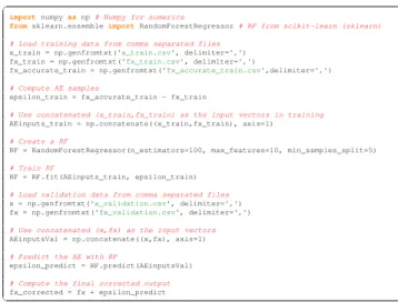
In this paper, we use an open source machine learning library scikit-learn1 for Python (Pedregosa et al., 2011) to implement the RF. In the scikit-learn library, the RF used for regression is named asRandomForestRegressor. In this paper, we study the effect of three different
RandomFore-stRegressor training parameters on the RF accuracy. These
three parameters aren_estimators, the number of trees in the forest,max_features, the number of input variables to con-sider when looking for the best split, andmin_samples_split, the minimum number of training samples required to split a node. For all the otherRandomForestRegressorparameters, the default values are used. An example code listing for train-ing and evaluattrain-ing the RF with the scikit-learn is given in Fig. 2.
1version 0.14.1, http://scikit-learn.org/
❉✐s❝✉ss✐♦♥
P
❛♣
❡r
⑤
❉✐s❝✉ss✐♦♥
P
❛♣
❡r
⑤
❉✐s❝✉ss✐♦♥
P
❛♣
❡r
⑤
❉✐
s❝✉ss
✐♦♥
P
❛♣
❡r
⑤
✞
importnumpyasnp# Numpy for numerics
fromsklearn.ensembleimportRandomForestRegressor# RF from scikit-learn (sklearn)
# Load training data from comma separated files
x_train = np.genfromtxt('x_train.csv', delimiter=',')
fx_train = np.genfromtxt('fx_train.csv', delimiter=',')
fx_accurate_train = np.genfromtxt('fx_accurate_train.csv',delimiter=',')
# Compute AE samples
epsilon_train = fx_accurate_train - fx_train
# Use concatenated (x_train,fx_train) as the input vectors in training AEinputs_train = np.concatenate((x_train,fx_train), axis=1) # Create a RF
RF = RandomForestRegressor(n_estimators=100, max_features=10, min_samples_split=5) # Train RF
RF = RF.fit(AEinputs_train, epsilon_train) # Load validation data from comma separated files
x = np.genfromtxt('x_validation.csv', delimiter=',')
fx = np.genfromtxt('fx_validation.csv', delimiter=',')
# Use concatenated (x,fx) as the input vectors AEinputsVal = np.concatenate((x,fx), axis=1) # Predict the AE with RF
epsilon_predict = RF.predict(AEinputsVal) # Compute the final corrected output fx_corrected = fx + epsilon_predict
✌
✝ ✆
Fig. 2. An example code listing for training and evaluating an RF model in scikit-learn.
3 Cloud droplet formation parameterization
Formation of cloud droplets in the atmosphere is a dynam-ical process affected by local meteorology and aerosol par-ticles acting as cloud condensation nuclei. In the most so-phisticated parameterizations, CDNC is calculated based on aerosol particle size distribution and chemical composition, pressure, temperature and vertical velocity of air parcel form-ing the cloud (Abdul-Razzak et al., 1998; Abdul-Razzak and Ghan, 2000, 2002; Nenes and Seinfeld, 2003; Fountoukis and Nenes, 2005).
The simulations in this study are conducted using the SALSA sectional aerosol model developed for atmospheric models (Kokkola et al., 2008; Bergman et al., 2012). In SALSA, aerosol size distribution is divided to different sub-ranges based on the particle size (3–50, 50–700, and 700– 10 000 nm). The size resolution differs between the sub-ranges depending on how sensitive the aerosol processes are to particle sizes of given subrange. In this study, the size sections within subranges have a constant volume ratio be-tween the adjacent sections. When using the default setup of SALSA, it has 10 size sections divided so that there are 3 sec-tions in the first subrange, 4 in the second subrange, and 3 in the third subrange. A more detailed description of the model is given by Kokkola et al. (2008).
Table 1.The numbers and names of the input variables in the ARG parameterizations.
Parameterization input variable name Number of variables Number of variables Number of variables in 4 size sections 7 size sections 70 size sections parameterization parameterization parameterization
Temperature 1 1 1
Pressure 1 1 1
Vertical velocity 1 1 1
Particle number concentration 8 13 130
Volume concentration of sulphate 8 13 130
Volume concentration of organic carbon 2 4 40
Volume concentration of dust 8 13 130
Total number of variables 29 46 433
take into account CDNC affecting processes within cloud, e.g. entrainment and as such is not a complete representation of CDNC. Also, we are omitting the first subrange as usually the cloud droplet nucleation in the atmosphere is not affected by these particles as they are too small to act as cloud con-densation nuclei. For simplicity, in this study we have also assumed that aerosol is composed of only one highly hygro-scopic compound (sulphate), one slightly hygrohygro-scopic com-pound (organic carbon) and one non-hygroscopic comcom-pound (dust).
Beyond evaluating the size resolution effect, we also study if the RF can be used to minimise the parameterization er-rors caused by the ARG parameterization itself in the estima-tion of CDNC. For that purpose we use an air parcel model, that solves the differential equations describing the aerosol growth to cloud droplets by water uptake in an adiabatically ascending air parcel. The model used has been described in detail elsewhere (Kokkola et al., 2003) and it has been used in several aerosol cloud interaction studies (e.g. Ro-makkaniemi et al., 2005, 2012). In the model, the differential equations are solved using an ordinary differential equation solver DLSODE (www.netlib.org), which solves initial-value problems for stiff or non-stiff ordinary differential equations using backward differentiation formulae. The liquid phase thermodynamics needed for the vapour pressures on the liq-uid particle surfaces are calculated with AIM, which is a chemical equilibrium code (Clegg et al., 1998). The aerosol size distribution is represented by the method of moving sec-tions, with 250 sections in this study. In the current study the model is used in its simplest setup, where only the condensa-tion of water is taken into account without other microphys-ical processes.
4 Models, simulations and results
4.1 Accurate and reduced models
Letf (x)∈Rdenote the numerically convergent computa-tional ARG cloud droplet formation parameterization that
Table 2.Size section configurations of the cloud droplet formation parameterizations used in simulations.
Total number Size sections in the Size sections in the of size sections diameter range diameter range
in the model 50–700 nm 0.7–10 µm
70 40 30
7 4 3
4 2 2
computes the value of the CDNC for the given inputx. By numerically convergent, it is meant that the output of the parameterization do not significantly change if more size sections were added. The input parameter vector x con-tains aerosol particle size and composition distributions, ver-tical velocity, pressures and temperature information. For the names and number of input variables in different parame-terizations see Table 1. In the following computations, the number of size sections for the representation of the particle size distributions is 70, see Table 2. With this discretization, the average simulation time of the accurate model is about 0.92 ms.
In the parameter vectorx˜of the reduced modelf (˜ x˜), the number of size sections for the aerosol particle size distribu-tions have been significantly reduced. We consider two dif-ferent levels of model reduction. In the first one, the number of size sections is 7 and in the second one 4, see Table 2. The average computation times are about 0.11 and 0.07 ms for the 7 and 4 sections parameterizations, respectively. Thus, when reducing from 70 size sections to 7 or 4 sections the aver-age reductions in computation times are about 89 and 93 %, respectively.
4.2 Construction of the RF predictor model
2092 A. Lipponen et al.: Correction of approximation errors with RF
Table 3.The prior probability distribution models used for the cloud droplet formation parameterization inputs. TheU,N, andŴdenote the uniform, Gaussian and gamma distributions, respectively. The details of the probability distribution functions are shown in Table 4.
Variable Distribution Unit
w Ŵ(1.25,0.75) m s−1
p U(10 000,100 000) P T U(240,300) K
ntot,1 Ŵ(2,800) cm−3
µ1 U(50,80) nm
σ1 N(1.5,0.125)
ntot,2 Ŵ(3,200) cm−3
µ2 U(100,200) nm
σ2 N(1.5,0.125)
ntot,3 Ŵ(1.25,0.75) cm−3
µ3 U(500,1500) nm
σ3 N(1.5,0.125)
prior probability distribution models, which were selected so that the realisations are plausible representations of their val-ues in the nature. The aerosol particle number distribution
n=n(d), whered is the diameter of the particle, was mod-elled as a sum of three log-normal modes representing the Aitken, accumulation and coarse mode aerosols:
n(d)=
3
X
i=1
ni(d) (5)
where each of the modes was modelled by
ni(d)=
ntot,i
d
q
2π (log(σi))2 exp
n
−(log(d/µi))2/
2σi2
o (6)
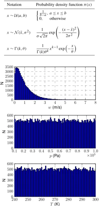
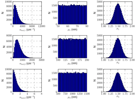
where thentot,i is the total number of particles in modei, andσi andµi the shape and log-scale parameters of modei. The parameters of the prior probability distribution models used in the generation of the vertical velocityw, pressurep, temperatureT, and the particle number distribution parame-terni,σi,µi samples are shown in Table 3 and the respec-tive probability density functions are shown in Table 4. The histograms of the temperature, pressure and vertical veloc-ity samples, and the particle number distribution parameters in the training sample set{xk}are shown in Figs. 3 and 4, respectively. The aerosol particle volume size distributions were constructed with the particle number distributions of the modes and randomly distributed volume fractions of each compound. The volume fractions for the sulphate were drawn from an uniform distributionU(0.01,1)separately for each mode. Further, the fractions of dust and organic carbon were drawn from uniform distributions such that the sum of the compound fractions was 1.
Table 4.The notations used for the probability distributions and their probability density functions.Ŵ(k)denotes the Gamma func-tion.
Notation Probability density functionπ(x)
x∼U(a, b)
1
b−a, a≤x≤b 0, otherwise
x∼N(x, σ¯ 2) 1
σ√2πexp − (x− ¯x)2
2σ2 !
x∼Ŵ(k, θ ) 1 Ŵ(k)θkx
k−1
exp
−x
θ
0 1 2 3 4 5 6 7 8
w(m/s) 0
500 1000 1500 2000 2500 3000 3500
N
0.1 0.2 0.3 0.4 0.5 0.6 0.7 0.8 0.9 1.0
p(Pa) ×105
0 100 200 300 400 500 600
N
240 250 260 270 280 290 300
T (K)
0 100 200 300 400 500 600
N
Fig. 3.Histograms of vertical velocityw, pressurepand temper-atureT in the sample set used for constructing the approximation error samples.Ndenotes the number of samples.
0 4000 8000 12000 ntot,1(cm
−3) 0
2000 4000 6000 8000 10000
N
50 60 70 80
µ1(nm)
0 500 1000 1500
N
1.00 1.25 1.50 1.75 2.00 σ1
0 1000 2000 3000 4000 5000
N
0 1000 2000 3000
ntot,2(cm
−3) 0
2000 4000 6000 8000
N
100 125 150 175 200 µ2(nm)
0 500 1000 1500
N
1.00 1.25 1.50 1.75 2.00 σ2
0 1000 2000 3000 4000 5000
N
0 2 4 6 8
ntot
,3(cm
−3) 0
2000 4000 6000 8000 10000
N
500 750 1000 1250 1500 µ3(nm)
0 500 1000 1500
N
1.00 1.25 1.50 1.75 2.00 σ3
0 1000 2000 3000 4000 5000
N
Fig. 4.Histograms for number concentrations of particlesni, scale parametersµi and shape parametersσi for the log-normal modesi = 1,2,3.Ndenotes the number of samples.
(a)
0 500 1000 1500 2000 2500 3000 3500 4000
f(x)(cm−3)
0 500 1000 1500 2000 2500 3000 3500 4000
˜f(˜x
)
(cm
−
3)
(b)
0 500 1000 1500 2000 2500 3000 3500 4000
f(x)(cm−3
) 0
500 1000 1500 2000 2500 3000 3500 4000
˜f(˜
x
)
(cm
−
3)
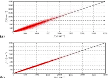
Fig. 5.Cloud droplet number concentrations (CDNC) computed with the approximate modelf (˜x˜)as functions of CDNCs given by the accurate modelf (x).(a)Approximate parameterization with 4 size sections for the aerosol particle size distributions.(b) Approx-imate parameterization with 7 size sections for the aerosol particle size distributions. Black solid lines represent the identity lines.
lower CDNC with the smaller number of size sections is the lower maximum supersaturation when using the ARG para-meterization.
Given the samples{xk}, the realisations of the approxima-tion error were simulated as
{ǫk=f′(xk)− ˜f′(P (xk)) , k=1, . . . , N}. (7) where f′(xk)=log(f (xk)) and f˜′(P (xk))= logf (P (˜ xk))
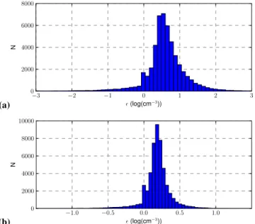
. It was found that the use of linear or logarithmic scale for the CDNC in the RF training resulted in similar root-mean-square errors and bias in the estimates. In some RF models, however, the mean relative error was more than ten times higher with the linear scale than with the logarithmic scale. Therefore, we chose to use CDNC with logarithmic scale in the computations. The histograms of the approximation errorsǫfor both the 7 and 4 size sections parameterizations are shown in Fig. 6.
Finally, the sample sets {xk,f˜′(P (xk))} and {ǫk} were used as the RF training set inputs and outputs, respectively, and the RF models were trained as described in the Sect. 2.3. Also here, the addition of logarithms of the coarse parame-terization outputs in the training set slightly improved the RF model accuracy and was therefore used. Once the RF pre-dictorg˜was constructed, the output of the accurate simulator
f (x)was approximated with
f (x)≈exp logf˜ x˜
+ ˜gx˜,f˜ x˜
2094 A. Lipponen et al.: Correction of approximation errors with RF
(a)
−3 −2 −1 0 1 2 3
ǫ(log(cm−3))
0 2000 4000 6000 8000
N
(b)
−1.0 −0.5 0.0 0.5 1.0
ǫ(log(cm−3))
0 2000 4000 6000 8000 10000
N
Fig. 6.Histograms of the approximation errorsǫ(x).Ndenotes the number of samples.(a)Approximate parameterization with 4 size sections for the aerosol particle size distributions.(b)Approximate parameterization with 7 size sections for the aerosol particle size distributions.
4.3 Results
4.3.1 Compensation of approximation errors due to
reduced coarse sectional representation of the aerosol size distribution
To evaluate the proposed approach, multiple RF predic-tor models for the approximation errors corresponding to both approximate ARG parameterizations, with 7 and 4 size sections, were constructed with different RF train-ing parameters. All possible combinations of parameter sets {25,50,100,200,400},{5,10,15,25}, and{2,5,15,25,100}
for n_estimators, max_features and min_samples_split,
re-spectively, were used. These parameter ranges were selected based on a test which showed that selecting values out-side these ranges either resulted in poor model accuracy or considerably larger computational burden with no signifi-cant improvement on the model accuracy. To avoid overop-timistic results, the constructed AE models were evaluated with a separate validation set of 25 000 samples of ARG model inputs. The validation set was sampled similarly as the training set but the samples were not included in the training of the RF model.
All predictor models were evaluated using the validation set, and the root-mean-squared error (RMSE) ǫRMSE and
mean relative error (MRE)ǫMREestimates were computed.
The error estimates were computed as
ǫRMSE=
v u u t 1
N N X
i=1
f (xi)− ˆf x˜i 2
,
ˆ
f (x˜)=exp logf˜ x˜
+ ˜gx˜,f˜ x˜
(9) and
ǫMRE=
1
N N X
i=1
|f (xi)− ˆf (x˜i)| |f (xi)|
. (10)
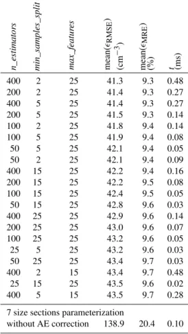
As the construction of an RF model is random, the tests were repeated 25 times for each AE model to also evaluate the ran-dom variations in the results. The average RMSE and MRE, average computation time of the approximation error model, and the model parameters for both of the approximate param-eterizationsf (˜x˜)corresponding to 20 different combinations of RF training parameters (n_estimators,max_features, and
min_samples_split) are given in Table 5 for the
parameteriza-tion with 7 size secparameteriza-tions and Table 6 for the parameterizaparameteriza-tion with 4 size sections. Complete results tables are given in the supplementary material of the paper. The bottom row in both Tables gives the respective errors between the accurate para-meterizationf (x)and reduced parameterizationf (˜x˜) with-out approximation error correction. The CDNC values com-puted with the accurate parameterizationf (xj)as a function of the AE corrected CDNC values using the predictorg˜with the lowest RMSE error are shown in Fig. 7. Panel a shows the case for the reduced model with 4 size sections and panel b the case with 7 size sections for the particle size distributions. The results show that by using the AE correction with the RF predictor model, both the RMSE and MRE errors are significantly decreased. In the case of the reduced pa-rameterization f (˜x˜) with 7 size sections, the RF training parameter selectionsn_estimators=400,max_features=2,
andmin_samples_split=25 resulted in the overall model in
which both the RMSE and MRE were the smallest. Here, the approximation error correction decreased the RMSE and the MRE to values less than 30 and 50 %, respec-tively, of the RMSE and MRE values of the CDNC com-puted without the approximation error correction. In the case of the reduced parameterizationf (˜x˜)with 4 size sec-tions, the lowest RMSE was obtained with the RF train-ing parameters n_estimators=400, max_features=2, and
min_samples_split=15. Also here, both the RMSE and
Table 5. Training parameters and results of the AE correc-tion in the case of 7 size seccorrec-tions parameterizacorrec-tion: number of trees in the RF modeln_estimators, the RF training parameters
min_samples_split, and max_features, the mean values of
root-mean-squared errorsǫRMSE(RMSE) and mean relative errorsǫMRE
(MRE), and the average time used for evaluating the RF modelt.
n_estimator
s
min_samples_split max_featur
es
mean(
ǫRMSE
)
(cm
−
3)
mean(
ǫMRE
)
(%) t (ms)
400 2 25 41.3 9.3 0.48
200 2 25 41.4 9.3 0.27
400 5 25 41.4 9.3 0.27
200 5 25 41.5 9.3 0.14
100 2 25 41.8 9.4 0.14
100 5 25 41.9 9.4 0.08
50 5 25 42.1 9.4 0.05
50 2 25 42.1 9.4 0.09
400 15 25 42.2 9.4 0.16
200 15 25 42.2 9.5 0.08
100 15 25 42.4 9.5 0.05
50 15 25 42.8 9.6 0.03
400 25 25 42.9 9.6 0.14
200 25 25 43.0 9.6 0.07
100 25 25 43.2 9.6 0.05
25 5 25 43.2 9.6 0.03
50 25 25 43.4 9.7 0.03
400 2 15 43.4 9.7 0.48
25 15 25 43.5 9.6 0.02
400 5 15 43.5 9.7 0.28
7 size sections parameterization
without AE correction 138.9 20.4 0.10
The mean of the CDNC values computed with the 70 size sections parameterization: 574.8 cm−3.
The standard deviation of the CDNC values computed with the 70 size sections parameterization: 509.5 cm−3.
The results also show that the RF model training pa-rameters did not significantly affect the accuracy of the AE model. The RF training parameter affecting the accu-racy of the model most wasmax_features. The randomness in the RF model training caused only minor variations in the resulting RF models showing the robustness of the ap-proach. As an example, in the 7 size sections AE corrected model with the RF training parametersn_estimators=400,
min_samples_split=2, and max_features=25, the RMSE
and the MRE varied between values 41.2–41.4 cm−3 and 9.23–9.28 %, respectively.
The average times to simulate the AE models varied be-tween 0.02 and 0.48 ms in the case of 7 size sections parame-terization and between 0.02 and 0.49 ms in 4 size sections pa-rameterization on a standard desktop computer. The average time to simulate the reduced modelf (˜x˜)with 7 and 4 size
Table 6.Training parameters and results of the AE correction in the case of 4 size sections parameterization: number of trees in the RF modeln_estimators, the RF training parametersmin_samples_split
and max_features, the mean values of root-mean-squared errors
ǫRMSE(RMSE) and mean relative errorsǫMRE(MRE), and the
av-erage time used for evaluating the RF modelt.
n_estimator
s
min_samples_split max_featur
es
mean(
ǫRMSE
)
(cm
−
3)
mean(
ǫMRE
)
(%) t (ms)
400 2 15 95.5 23.5 0.48
400 5 15 95.7 23.5 0.26
200 2 15 95.9 23.6 0.26
200 5 15 96.1 23.5 0.13
400 2 25 96.7 23.1 0.49
100 2 15 96.8 23.7 0.14
100 5 15 96.9 23.7 0.08
200 2 25 97.2 23.2 0.26
100 2 25 97.3 23.3 0.14
200 5 25 97.9 23.2 0.13
50 5 15 98.2 23.8 0.05
50 2 15 98.4 24.0 0.08
400 5 25 98.6 23.1 0.26
400 15 15 98.8 24.0 0.16
200 15 15 99.2 24.1 0.08
100 5 25 99.4 23.3 0.08
50 5 25 99.6 23.5 0.05
100 15 15 99.8 24.2 0.05
400 2 10 99.8 24.6 0.48
200 2 10 100.1 24.6 0.26
4 size sections parameterization
without AE correction 341.1 54.6 0.06
The mean of the CDNC values computed with the 70 size sections parameterization: 574.8 cm−3.
The standard deviation of the CDNC values computed with the 70 size sections parameterization: 509.5 cm−3.
sections were about 0.10 and 0.06 ms, respectively. These AE model running times for computingf (ˆx˜)resulted in overall average runtimes of 0.12–0.58 ms for the 7 size sections and 0.08–0.54 ms for the 4 size sections AE corrected parame-terizations. Thus, the reduction in computation times of the approximation error corrected modelsf (ˆx˜)is in the range of 37–91 % compared to the run time of the accurate model
2096 A. Lipponen et al.: Correction of approximation errors with RF
(a)
0 500 1000 1500 2000 2500 3000 3500 4000
f(x)(cm−3)
0 500 1000 1500 2000 2500 3000 3500 4000
ˆf(˜x
)
(cm
−
3)
(b)
0 500 1000 1500 2000 2500 3000 3500 4000
f(x)(cm−3)
0 500 1000 1500 2000 2500 3000 3500 4000
ˆf(˜x
)
(cm
−
3)
Fig. 7.Cloud droplet number concentrations (CDNC) computed with the approximation error corrected parameterizationf (ˆ x˜j)as functions of CDNCs given by the accurate parameterizationf (xj).
(a)Reduced parameterizationf (˜x˜)with 4 size sections for the rep-resentation of the aerosol particle size distributions.(b)Reduced parameterizationf (˜x˜)with 7 size sections for the representation of the aerosol particle size distributions. Black solid lines represent the identity lines.
of, for example, the RF predictor model with the training parametersn_estimators=25,min_samples_split=15, and
max_features=25 resulted in the overall model with only
slightly larger (about 0.3 %) MRE error and 0.46 ms faster running time compared to the RF model with the smallest MRE error in the case of 7 size sections parameterization. Notice that the computation time of the error prediction by the RF model is independent of the computation times off
orf˜. Thus, the relative time saving by the proposed approach will increase as the computation time off increases.
4.3.2 Compensation of approximation errors due to
reduction of process model internal numerics
In addition to the coarse sectional representation of the the aerosol particle distribution as the approximation error source, also simulations with an air parcel modelh(xj)as the accurate model were carried out (see Sect. 3 for the descrip-tion ofh(xj)). In these simulations, the 7 size sections ARG parameterization was used as the approximative model. The same training and validation datasets as in the previous ARG parameterization simulations were used and an RF model with parameters n_estimators=400, min_samples_split=
2, andmax_features=25 was trained to predict the approx-imation errors. The CDNC values computed with and with-out the approximation error correction as functions of CDNC values of the air parcel model h(xj)are shown in Fig. 8. With the approximation error correction, the decrease of the errors was significant, the RMSE decreased from 206.5 to 93.3 cm−3 (the mean of the CDNC values computed with
(a)
0 500 1000 1500 2000 2500 3000
h(x)(cm−3)
0 500 1000 1500 2000 2500 3000
˜f(˜x
)
(cm
−
3)
(b)
0 500 1000 1500 2000 2500 3000
h(x)(cm−3
) 0
500 1000 1500 2000 2500 3000
ˆf(˜x
)
(cm
−
3)
Fig. 8.Cloud droplet number concentrations (CDNC) computed with the the approximate modelf (˜ x˜)(a)and the approximation error corrected parameterizationf (ˆx˜)(b)as functions of CDNCs given by the air parcel modelh(xj). Black solid lines represent the identity lines.
h(xj)was 452.7 cm−3) and the MRE from 36.6 to 12.6 %. The biases in the approximative model (Fig. 8a) and the AE corrected model (Fig. 8b) are 132 and 9.1 cm−3, respectively. These results show that the proposed AE compensation ap-proach is also capable of compensating the errors due to re-duction of the internal numerics of the process model.
5 Conclusions
Due to computational time and resource limitations related to atmospheric models, several physical processes have to be simulated using reduced models. The use of a reduced model, however, induces approximation errors to the simulation re-sults. In this study, we presented a novel approach to correct these approximation errors and applied it to the calculation of cloud droplet number concentration (CDNC). In the paper, the approximation errors (in CDNC) caused by coarse sec-tional representation of the aerosol particle distribution and the approximative ARG parameterization of aerosol activa-tion were studied.
In our approach, the approximation errors caused by model reduction are modelled as an additive approximation error noise process in the simulation model and the RF al-gorithm is utilised for construction of a predictor for the re-alisation of the approximation error for given model input parameters. This way the accurate simulation model can be approximated in a computationally fast form by evaluating the reduced model and the prediction of the approximation error.
significantly smaller errors in the CDNC calculation than us-ing the reduced model alone with a small increment in the computational cost. Also the systematic errors caused by re-duced model accuracy can be efficiently eliminated. Further it was noted that the use of CDNC in logarithmic scale in the RF training may have high impact on the MRE of the final CDNC estimates. In some cases, the MRE was more than ten times higher if the linear scale for the CDNC was used in the training instead of logarithmic scale.
Another significant result in this study was that if the num-ber of size sections were further decreased from 7 to 4, the RMS errors in the RF corrected CDNC of the 4 sections model were lower than the errors of the uncorrected 7 sec-tions model. This shows that the RF method could be useful in reducing the number of size distribution parameters, when aerosol models are developed for simulations of decades or centuries. As the method is in no way limited to sectional ap-proach, it could be applied for reducing number of modes in modal models. This type of model reduction has been con-sidered, for example, in Liu et al. (2012).
Here the RF method was employed in the calculation of CDNC with variables typical to atmospheric models. The method can be easily and efficiently extended to take ac-count more complex aerosol including for example surface active (Sorjamaa et al., 2004) or semi-volatile aerosol com-pounds (Romakkaniemi et al., 2005) by simply adding new variables to the training data. The method is highly efficient especially in the case of physical processes, which have been found to be difficult to parameterize with traditional meth-ods due to high dependence of the processes on several pa-rameters. For example in our simplest case in the calculation of cloud droplet formation, the number of parameters was 29 and thus finding for example analytic formulas for cor-rections are difficult. A possible topic of future studies is to test the proposed approach with some variant of the RF algo-rithm, such as the weighted RF (Chen et al., 2004). Further, the proposed approach is rather general and extension of it to different physical simulation models is a straightforward task.
Appendix A
ALGORITHMS
Algorithm 1: Simulation of training data.
Inputs:Accurate and approximative modelsf(x)andf˜(x˜), respectively, prior probability distribution modelπ(x)for the input variablex, model reduction mappingPand the number of samplesNto be used in the precomputation steps.Output:
Training data{x˜k,ǫk}for the RF model 1:fori=1, .., Ndo
2: Draw a random samplexi from the probability distributionπ(x)(or use sample from a set of measured realisations ofx).
3: Simulate the accurate model, i.e. computef(xi). 4: Simulate the approximate model, i.e. computef˜(P (xi)). 5: Add a sample(x˜i,ǫi)wherex˜i=P (xi)and
ǫi=f(xi)−f˜(P (xi))to the training set. 6:end for
Supplementary material related to this article is available online at http://www.geosci-model-dev.net/6/ 2087/2013/gmd-6-2087-2013-supplement.pdf.
Acknowledgements. The financial support by the Academy of
Finland (project 119270 and Centre of Excellence programmes 1118615 and 250215) and by the strategic funding of the University of Eastern Finland are gratefully acknowledged.
Edited by: A. Kerkweg
References
Abdul-Razzak, H., Ghan, S. J., and Rivera-Carpio, C.: A paramete-rization of aerosol activation 1. single aerosol type, J. Geophys. Res., 103, 6123–6131, doi:10.1029/97JD03735, 1998.
Abdul-Razzak, H. and Ghan, S. J.: A parameterization of aerosol activation 2. Multiple aerosol types, J. Geophys. Res., 105, 6837– 6844, doi:10.1029/1999JD901161, 2000.
Abdul-Razzak, H. and Ghan, S. J.: A parameterization of aerosol ac-tivation 3. Sectional representation, J. Geophys. Res., 107, AAC 1-1–AAC 1-6, doi:10.1029/2001JD000483, 2002.
Arridge, S., Kaipio, J., Kolehmainen, V., Schweiger, M., Somersalo, E., Tarvainen, T., and Vauhkonen, M.: Approx-imation errors and model reduction with an application in optical diffusion tomography, Inverse Probl., 22, 175–195, doi:10.1088/0266-5611/22/1/010, 2006.
Bechtel, B. and Daneke, C.: Classification of local climate zones based on multiple earth observation data, IEEE J. Sel. Top. Appl., 5, 1191–1202, doi:10.1109/JSTARS.2012.2189873, 2012. Bergman, T., Kerminen, V.-M., Korhonen, H., Lehtinen, K. J.,
2098 A. Lipponen et al.: Correction of approximation errors with RF
ECHAM5-HAM aerosol-climate model, Geosci. Model Dev., 5, 845–868, doi:10.5194/gmd-5-845-2012, 2012.
Breiman, L.: Random Forests, Mach. Learn., 45, 5–32, doi:10.1023/A:1010933404324, 2001.
Chen, C., Liaw, A., and Breiman, L.: Using random forests to learn imbalanced data, Technical Report 666, Statistics Department of University of California, Berkeley, USA, 2004.
Clegg, S. L., Brimblecombe, P., and Wexler, A. S.: Thermodynam-ical model of the system H+-NH+4-SO24−-NO−3-H2O at tropo-spheric temperatures, J. Phys. Chem. A, 102, 2137–2154, 1998. Forster, P., Ramaswamy, V., Artaxo, P., Berntsen, T., Betts, R.,
Fa-hey, D., Haywood, J., Lean, J., Lowe, D., Myhre, G., Nganga, J., Prinn, R., Raga, G., Schulz, M., and Van Dorland, R.: Changes in atmospheric constituents and in radiative forcing, in: Cli-mate Change 2007: The Physical Science Basis, Contribution of Working Group I to the Fourth Assessment Report of the Inter-governmental Panel on Climate Change, edited by: Solomon, S., Qin, D., Manning, M., Chen, Z., Marquis, M., Averyt, K., Tig-nor, M., and Miller, H., Cambridge University Press, Cambridge, UK and New York, NY, USA, 2007.
Fountoukis, C. and Nenes, A.: Continued development of a cloud formation parameterization for global climate models, J. Geo-phys. Res., 110, D11212, doi:10.1029/2004JD005591, 2005. Haykin, S. O.: Neural networks and learning machines, Prentice
Hall, New York, 2009.
Jacobson, M. Z.: GATOR-GCMM: a global through urban scale air pollution and weather forecast model. 1. Model design and treatment of subgrid soil, vegetation, roads, rooftops, wa-ter, sea ice, and snow, J. Geophys. Res., 106, 5385–5402, doi:10.1029/2000JD900560, 2001.
Kaipio, J. and Somersalo, E.: Statistical and Computational Inverse Problems, Springer, New York, 2005.
Kokkola, H., Romakkaniemi, S., Kulmala, M., and Laaksonen, A.: A cloud microphysics model including trace gas condensation and sulfate chemistry, Boreal Environ. Res., 8, 413–424,2003. Kokkola, H., Korhonen, H., Lehtinen, K. E. J., Makkonen, R.,
Asmi, A., Järvenoja, S., Anttila, T., Partanen, A.-I., Kulmala, M., Järvinen, H., Laaksonen, A., and Kerminen, V.-M.: SALSA – a Sectional Aerosol module for Large Scale Applications, At-mos. Chem. Phys., 8, 2469–2483, doi:10.5194/acp-8-2469-2008, 2008.
Kolehmainen, V., Schweiger, M., Nissilä, I., Tarvainen, T., Ar-ridge, S., and Kaipio, J.: Approximation errors and model reduc-tion in three-dimensional diffuse optical tomography, J. Opt. Soc. Am. A, 10, 2257–2267, doi:10.1364/JOSAA.26.002257, 2009. Kolehmainen, V., Tarvainen, T., Arridge, S., and Kaipio, J.:
Marginalization of uninteresting distributed parameters in in-verse problems – application to diffuse optical tomography, International Journal for Uncertainty Quantification, 1, 1–17, doi:10.1615/Int.J.UncertaintyQuantification.v1.i1.10, 2011. Lehikoinen, A., Finsterle, S., Voutilainen, A., Heikkinen, L.,
Vauhkonen, M., and Kaipio, J.: Approximation errors and truncation of computational domains with application to geophysical tomography, Inverse Probl. Imag., 1, 371–389, doi:10.3934/ipi.2007.1.371, 2007.
Liu, X., Easter, R. C., Ghan, S. J., Zaveri, R., Rasch, P., Shi, X., Lamarque, J.-F., Gettelman, A., Morrison, H., Vitt, F., Con-ley, A., Park, S., Neale, R., Hannay, C., Ekman, A. M. L., Hess, P., Mahowald, N., Collins, W., Iacono, M. J.,
Brether-ton, C. S., Flanner, M. G., and Mitchell, D.: Toward a min-imal representation of aerosols in climate models: description and evaluation in the Community Atmosphere Model CAM5, Geosci. Model Dev., 5, 709–739, doi:10.5194/gmd-5-709-2012, 2012.
Munro, N. P., Cairns, D. A., Clarke, P., Rogers, M., Stanley, A. J., Barrett, J. H., Harnden, P., Thompson, D., Eardley, I., Banks, R. E., and Knowles, M. A.: Urinary biomarker profiling in tran-sitional cell carcinoma, Int. J. Cancer, 119, 2642–2650, 2006. Nenes, A. and Seinfeld, J.: Parameterization of cloud
dropletfor-mation in global climate models, J. Geophys. Res., 108, 4415, doi:10.1029/2002JD002911, 2003.
Nissinen, A., Heikkinen, L., Kolehmainen, V., and Kaipio, J.: Compensation of errors due to discretization, domain trunca-tion and unknown contact impedances in electrical impedance tomography, Meas. Sci. Technol., 20, 105504, doi:10.1088/0957-0233/20/10/105504, 2009.
Nissinen, A., Kolehmainen, V., and Kaipio, J.: Compensation of modelling errors due to unknown domain boundary in electri-cal impedance tomography, IEEE T. Med. Imaging, 30, 231–242, 2011.
Pal, M.: Random Forest classifier for remote sens-ing classification, Int. J. Remote Sens., 26, 217–222, doi:10.1080/01431160412331269698, 2005.
Pedregosa, F., Varoquaux, G., Gramfort, A., Michel, V., Thirion, B., Grisel, O, Blondel, M., Prettenhofer, P., Weiss, R., Dubourg, V., Vanderplas, J., Passos, A., Cournapeau, D., Brucher, M., Per-rot, M., and Duchesnay, E.: Scikit-learn: Machine Learning in Python, J. Mach. Learn. Res., 12, 2825–2830, 2011.
Rodriguez, M. and Dabdub, D. J.: IMAGES-SCAPE2: A model-ing study of size and chemically resolved aerosol thermodynam-ics in a global chemical transport model, J. Geophys. Res., 109, D02203, doi:10.1029/2003JD003639, 2004.
Rojas, R.: Neural Networks: A Systematic Introduction, Springer-Verlag, Berlin, 1996.
Romakkaniemi, S., Kokkola, H., and Laaksonen, A.: Parameteriza-tion of the nitric acid effect on CCN activaParameteriza-tion, Atmos. Chem. Phys., 5, 879–885, doi:10.5194/acp-5-879-2005, 2005.
Romakkaniemi, S., Arola, A., Kokkola, H., Birmili, W., Tuch, T., Kerminen, V.-M., Rïsänen, P., Smith, J. N., Korhonen, H., and Laaksonen, A.: Effect of aerosol size distribution changes on AOD, CCN and cloud droplet concentration: Case studies from Erfurt and Melpitz, Germany, J. Geophys. Res., in press, doi:10.1029/2011JD017091, 2012.
Sorjamaa, R., Svenningsson, B., Raatikainen, T., Henning, S., Bilde, M., and Laaksonen, A.: The role of surfactants in Köh-ler theory reconsidered, Atmos. Chem. Phys., 4, 2107–2117, doi:10.5194/acp-4-2107-2004, 2004.
Tesfamariam, S. and Liu, Z.: Earthquake induced damage classifica-tion for reinforced concrete buildings, Struct. Saf., 32, 154–164, doi:10.1016/j.strusafe.2009.10.002, 2010.
Weisenstein, D. K., Penner, J. E., Herzog, M., and Liu, X.: Global 2-D intercomparison of sectional and modal aerosol modules, At-mos. Chem. Phys., 7, 2339–2355, doi:10.5194/acp-7-2339-2007, 2007.