www.ann-geophys.net/26/167/2008/ © European Geosciences Union 2008
Annales
Geophysicae
Observed tail current systems associated with bursty bulk flows and
auroral streamers during a period of multiple substorms
C. Forsyth1, M. Lester1, S. W. H. Cowley1, I. Dandouras2, A. N. Fazakerley3, R. C. Fear1, H. U. Frey4, A. Grocott1,
A. Kadokura5, E. Lucek6, H. R`eme2, S. E. Milan1, and J. Watermann7
1Dept. Physics and Astronomy, University of Leicester, Leicester, LE1 7RH, UK
2CESR/CNRS, 9 Avenue du Colonel Roche, B.P. 4346, 31028, Toulouse Cedex 4, France
3Mullard Space Science Laboratory, University College London, Holmbury St. Mary, Dorking, Surrey, RH5 6NT, UK 4Space Sciences Laboratory, University of California, Berkeley, CA 94720, USA
5National Institute of Polar Research, 9-10-1 Kaga, Itabashi, Tokyo 173-8515, Japan 6Blackett Laboratory, Imperial College, London, SW7 2BZ, UK
7Atmosphere Space Research Division, Danish Meteorological Institute, Copenhagen, Denmark
Received: 26 March 2007 – Revised: 14 December 2007 – Accepted: 18 December 2007 – Published: 4 February 2008
Abstract. We present a multi-instrument study of a
sub-storm bursty bulk flow (BBF) and auroral streamer. During a substorm on 25 August 2003, which was one of a series of substorms that occurred between 00:00 and 05:00 UT, the Cluster spacecraft encountered a BBF event travelling Earth-wards and duskEarth-wards with a velocity of∼500 km s−1some nine minutes after the onset of the substorm. Coincident with this event the IMAGE spacecraft detected an auroral streamer in the substorm auroral bulge in the Southern Hemisphere near the footpoints of the Cluster spacecraft. Using FluxGate Magnetometer (FGM) data from the four Cluster spacecraft, we determine the field-aligned currents in the BBF, using the curlometer technique, to have been∼5 mA km−2. When pro-jected into the ionosphere, these currents give ionospheric field-aligned currents of∼18 A km−2, which is comparable with previously observed ionospheric field-aligned currents associated with BBFs and auroral streamers. The observa-tions of the BBF are consistent with the plasma “bubble” model of Chen and Wolf (1993). Furthermore, we show that the observations of the BBF are consistent with the creation of the BBF by the reconnection of open field lines Earthward of a substorm associated near-Earth neutral line.
Keywords. Magnetosphere (Auroral phenomena; Current
systems; Storms and substorms)
Correspondence to:C. Forsyth (cf50@ion.le.ac.uk)
1 Introduction
The current circuits of the magnetosphere-ionosphere system are a fundamental constituent of the near-Earth space envi-ronment. Whereas large scale current systems, such as the substorm current wedge, can excite auroral activity covering many hours of magnetic local time (MLT), localised current systems can excite localised auroral forms. Ground-based magnetometers and radars and low Earth orbiting spacecraft have previously been used to study the ionospheric current systems, but the launch of the Cluster mission in 2001 pro-vides a unique opportunity to study current systems out in the magnetosphere.
BXand the change inBY was negative (positive), the
space-craft passed through the duskward (dawnward) edge of the flow (Sergeev et al., 1996, Fig. 2) and vice versa beneath the plasma sheet. It should be noted that most definitions of BBFs (see e.g. Cao et al., 2006) consider multiple bursts of high speed plasma flow within a limited period (commonly 10 min) to be a single BBF. As such, we can apply the re-sults of Chen and Wolf (1993) and Sergeev et al. (1996) to individual flow bursts within a BBF.
In recent years, there have been a number of studies re-lating BBFs to auroral streamers either explicitly, with di-rect observation of both features (e.g. Lyons et al., 1999; Nakamura et al., 2001a,b), or implicitly, with ionospheric measurements being compared to the predicted form of the ionospheric manifestations of BBFs from the model of Chen and Wolf (1993) (e.g. Henderson et al., 1998; Amm et al., 1999; Sergeev et al., 2004). In particular, Nakamura et al. (2001a) dealt with the footprint location of the Geotail satel-lite and the comparison of Geotail observations of BBFs and the passage of the streamers near the spacecraft’s footprint. They found good spatial and temporal correlation between flow bursts in the tail and auroral activity. They also found that auroral enhancements that break up within the vicinity of the spacecraft footprint, calculated using the Hybrid In-put Algorithm (HIA) (Kubyshkina et al., 1999) to modify the magnetic field model of Tsyganenko (1989), appeared within ±1 min of the flow onset in the tail. It should be noted that in the study by Nakamura et al. (2001a), the variations in the footpoint location from the different models tended to be in the north-south direction as opposed to a change in the MLT. Studies of ionospheric current systems near the footpoints of BBFs and associated with auroral streamers have shown that they are also consistent with the Chen and Wolf (1993) model (Amm et al., 1999; Sergeev et al., 2004; Nakamura et al., 2005). Combined ground and space-based studies of the ionosphere during the passage of auroral streamers have shown that the bright westward edge of the streamer is associated with a large, upward field-aligned current den-sity whereas diffuse aurora to the east is associated with a lower, Earthward current density (Amm et al., 1999; Sergeev et al., 2004), although a lack of tail observations meant that these streamers could not be directly associated with bursty bulk flows. Amm et al. (1999) inferred field-aligned currents in streamers of ∼25 A km−2 by using the method of char-acteristics (Inhester et al., 1992; Amm, 1995, 1998) to in-vert ground magnetic field data and ionospheric electric field data. This forward technique solves a 2-D partial differential equation along its characteristics for the Hall conductance, allowing other electrodynamic parameters to be inferred with the inclusion of the measurements. Grocott et al. (2004) es-timated an ionospheric field-aligned current of∼0.2 A km−2 near the footpoint of the Cluster spacecraft as the spacecraft detected the passage of a BBF during a “quiet” period, by measuring the curl of the ionospheric flows detected by the CUTLASS radars (Lester et al., 2004) and assuming a
non-substorm Pedersen conductivity of a few Siemens. They showed that this current system was associated with auro-ral activity with a maximum brightness of∼1 kR, although they did not discuss the current system in terms of the Chen and Wolf (1993) model. Nakamura et al. (2005) inferred the curl of the ionospheric equivalent currents near the footpoint of the Cluster spacecraft at the time of a BBF using the 2-D spherical elementary current technique of Amm and Vil-janen (1999) to invert IMAGE magnetometer data. In the case of uniform conductances within the region of the Clus-ter footpoint, this gave field-aligned currents of the order of 3 A km−2. However, no auroral data were presented such that the passage of an auroral streamer could not be con-firmed. Also, EISCAT radar data indicated that there were localised conductance enhancements, although the localised feature was considered not to affect the overall current pat-tern. The currents observed in these studies vary by two or-ders of magnitude, although the three values were obtained during differing periods of auroral, magnetic and substorm activity, indicating that the substorm phase during which the BBF is detected has a strong influence on the associated cur-rents. A review of the ionospheric signatures of BBFs is given by Amm and Kauristie (2002).
On 25 August 2003, the Cluster spacecraft observed a BBF consisting of two flow bursts during a period of mul-tiple substorms. Simultaneously, the IMAGE spacecraft ob-served an auroral streamer in the Southern Hemisphere auro-ral oval. We show that the field-aligned currents detected by the Cluster spacecraft, calculated using the curlometer tech-nique (Dunlop et al., 1988; Robert et al., 1998, and references therein), are consistent with previous ground-based studies of ionospheric currents detected in association with an auroral streamer by Amm et al. (1999). The pitch angle distribu-tion, energy spectra of particles, ion density and magnetic flux within the flow are shown to be consistent with the re-connection of open field lines close to the spacecraft.
2 Instrumentation
dawn and Cluster 2 (green) was closest to dusk. Cluster 3 (yellow) was furthest down tail. At 01:00 UT Cluster 1 was located at [−18.62,−3.58,−0.96]REand the average
separa-tion of the spacecraft was 120 km. Cluster data are presented here from the FluxGate Magnetometer (FGM; Balogh et al., 2001), the Cluster Ion Spectrometer CODIF sensor (CIS; R`eme et al., 2001), and the Plasma Electron And Current Experiment High Energy Electron Analyser (PEACE HEEA; Johnstone et al., 1997). The FGM data presented is based on the full resolution (22 Hz) data from the Cluster Active Archive. These data have been calibrated such that they are better suited to the multi-spacecraft analysis presented within this study. Plots of the data from the PEACE HEEA sensor also include a trace of the spacecraft potential, as measured by the Electric Fields and Waves instrument (EFW; Gustafs-son et al., 2001).
The IMAGE spacecraft passed through perigee at around 23:30 on 24 August 2003 and was travelling sunward and duskward during the interval, passing over the southern mag-netic pole shortly after midnight. Data is presented from the Far-UltraViolet Wideband Imaging Camera (FUV-WIC; Mende et al., 2000a,b) on board IMAGE.
Interplanetary magnetic field and solar wind data were obtained by the Advanced Composition Explorer spacecraft (ACE; Stone et al., 1998) located in the solar wind upstream of the Earth at [227,−26,15]RE GSM. Data are employed
from the magnetometer (MAG; Smith et al., 1998) and So-lar Wind Electron Proton Alpha Monitor (SWEPAM; McCo-mas et al., 1998) instruments. The data have been lagged by 44 min to the magnetopause using the method of Khan and Cowley (1999), with an uncertainty of±3 min.
Ground-based magnetometer data are presented from the west coast magnetometer stations of the Greenland mag-netometer chain operated by the Danish Meteorological Institute (DMI) (for instrument details, see http://www. dmi.dk/projects/chain/greenland.html) and from the Antarc-tic low power magnetometer (LPM) chains operated by the British Antarctic Survey (BAS) and the Japanese Na-tional Institute for Polar Research (NIPR) (for instru-ment details, see http://www.antarctica.ac.uk/bas research/ instruments/lpm.php). Figure 2 indicates the locations of these magnetometer stations in MLT-invariant latitude mag-netic coordinates at 01:16 UT on 25 August 2003 from alti-tude adjusted corrected geomagnetic coordinates (AACGM) (Baker and Wing, 1989). The magnetic footpoint of the Clus-ter spacecraft, calculated using the T96 model, is shown as a red star in each panel.
3 Observations
3.1 Cluster observations
Data from the Cluster FGM and CIS instruments from Clus-ter 4 between 01:00 and 02:00 UT, encompassing the
sub-5 0 -5 -10 -15 -20 -25 XGSM
15 10 5 0 -5 -10 -15
YGSM
5 0 -5 -10 -15 -20 -25 XGSM
-15 -10 -5 0 5 10 15
ZGSM
-15 -10 -5 0 5 10 15 YGSM
-15 -10 -5 0 5 10 15
ZGSM
Cluster 1 (Rumba)
Cluster 2 (Salsa)
Cluster 3 (Samba)
Cluster 4 (Tango)
00:00 U
T 01:0
0UT 02:00 UT
00:00 UT 01:00 T 02:00
0:00U
T
01:00 UT
02:00 UT
00:00 UT 01:00 UT
02:00 UT
00:00 UT
01:00 UT 02:00 UT
U U
(a)
(c)
(b)
T
Fig. 1. Plots of the Cluster and IMAGE orbital positions between 00:00, 01:00 and 02:00 UT in the(a)X-Y,(b)Y-Z and(c)X-Z in GSM coordinates. The Cluster tetrahedron is magnified by a factor of 200. Cluster 1 (Rumba, blue) is plotted at the correct location. The dotted lines represent the magnetic field lines passing through Cluster 1 at 00:00, 01:00 and 02:00 UT as determined by the Tsy-ganenko T96 model (TsyTsy-ganenko and Stern, 1996).
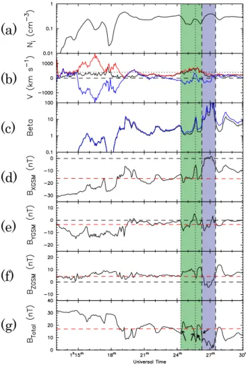
storm, are presented in Fig. 3. CIS data were unavailable from Cluster 1 and 2 and data from Cluster 3 were noisy and will not be discussed here. Discussion of ion moments from the CIS instrument on board Cluster 4 will refer to the proton moments derived from the CODIF sensor, since the proton densities detected by the CIS instrument were much larger than the densities of other ions. Differences in the FGM data from the four spacecraft are unnoticeable on the timescales presented here and as such, overall magnetic field conditions are taken to be those at Cluster 4. The FGM data have been smoothed using a 4 s Box Car filter. Figure 3a shows the ion density moments from the CIS instrument. Figure 3b–e shows the magnetic field components in the X, Y and Z GSM directions and the total magnetic field strength, respectively, from the FGM instrument. The red dashed line in Fig. 3b–e represents the T96 model magnetic field values at the loca-tion of the spacecraft. The vertical dashed line at 01:15 UT indicates the time at which Cluster first detected evidence of the substorm expansion phase, evidenced as a decrease in the total magnetic field of∼30 nT over the following 12 min, dominated by a decrease in theBXcomponent indicating a
dipolarisation of the magnetic field. The shaded area indi-cates the time at which Cluster encountered the BBF.
(a)
THL SVS KUV
UPN UMQ
GDH ATU STF SKT GHB
NRD
DMH DNB
SCO
FHB NAQ
AMK
(b)
M78-337
M79-336M81-338 M82-003 M83-348 M84-336M85-002
M85-096
M87-028 M87-068 M88-316
M68-041 M69-041 M70-039
M70-044M74-043 M77-040
Fig. 2. Maps indicating(a)the locations of the Greenland mag-netometer chain run by the Danish Meteorological Institute and(b)
the Antarctic low power magnetometer chains run by the British Antarctic Survey and the Japanese National Institute for Polar Re-search in MLT-invariant latitude coordinates calculated at 01:16 UT on 25 August 2003 from altitude adjusted corrected geomagnetic coordinates (12:00 MLT is at the top and 18:00 MLT to the left). The Cluster footpoint at this time is indicated by the red star. The radial dotted lines indicate hours of MLT, while the dotted concen-tric circles are shown for every 10◦of magnetic latitude.
(Fig. 3e) dropped by∼30 nT, dominated by a decline in the
BXcomponent (Fig. 3b). TheBZ component (Fig. 3d) was
elevated above that of the model field throughout most of the
(a)
(b)
(c)
(d)
(e)
Fig. 3. Stacked plots of the ion and magnetic field data from Clus-ter 4, showing(a)the ion density,(b–d)the X, Y, and Z components of the magnetic field in GSM coordinates, and(e)the total magnetic field value. The dashed lines represent the zero value in panels (b– e), while the red dashed line represents the T96 model field value. The vertical dashed line indicates the time at which Cluster 4 de-tected the substorm expansion phase. The shaded area indicates Cluster’s encounter with the BBF.
interval, which, coupled with the decrease in theBX
compo-nent, indicates that the field became more dipole-like at this time. This is taken to be an indication that the Cluster space-craft detected a substorm expansion phase onset at 01:15 UT. Since Cluster was initially in the southern lobe and moving away from the central plasma sheet, the plasma sheet config-uration changed so as to engulf the spacecraft.
conditions that the peak flow velocity perpendicular to the magnetic field,Vperp,>250 km s−1and thatβXY>2 (based
on the X and Y components of the magnetic field). We adapt the above to emphasise the convective element of the model such thatVperp>300 km s−1for the flow enhancement to be considered a BBF. Based on the prediction of the model of Chen and Wolf (1993) that the under-populated flux tubes that make up a BBF are convecting magnetic structures in which the magnetic field magnitude is enhanced, we distin-guish between flow bursts within the BBF based on the mag-netic field magnitude. We also compare the magmag-netic field data and ion density to distinguish between separate flow bursts. This differs from the definition given by Angelopou-los et al. (1992), who used the plasma flow data to define flow bursts.
At 01:24 UT, approximately 9 min after Cluster detected the substorm expansion phase, the spacecraft encountered a bursty bulk flow consisting of two flow bursts (indicated by the shaded region in Fig. 3) followed by a low magnetic field event in which the total magnetic field strength at Cluster dropped to∼1 nT . We now consider data from the Cluster spacecraft which illustrate the passage of the BBF and the subsequent low field event.
Presented in Fig. 4 are data from the FGM and CIS instru-ments between 01:18 and 01:30 UT. Figure 4a shows the ion density. Figure 4b shows the ion velocity perpendicular to the magnetic field (black), defined asb×(V×b)wherebis
the unit magnetic field vector andV is the ion velocity
vec-tor, the ion velocity parallel to the magnetic field (blue), and the total ion velocity(red). Figure 4c shows plasma beta (β, black) and the plasma beta calculated using only theBXand
BY GSM components (βXY, blue). Figure 4d–g shows the X,
Y and Z GSM components of the magnetic field and the total magnetic field strength, respectively. The green shaded area indicates the time at which the BBF engulfed Cluster. The horizontal dashed line in Fig. 4b–f indicates the zero value. The horizontal dotted line in Fig. 4b indicates 300 km s−1. The red dashed line in Fig. 4d–g represents the T96 model field value. The dotted vertical lines represent the start of each of the two flow bursts. The dashed vertical lines en-close the low field event.
Between 01:24:15 and 01:26:15 UT, the ion velocity per-pendicular to the magnetic field at Cluster (Fig. 4b) increased to >300 km s−1 with a peak value of ∼720 km s−1 and a mean value of∼500 km s−1. Simultaneously, the magnetic field strength increased in all components by∼5 nT indicat-ing that Cluster encountered a BBF. The ion density detected by Cluster at this time halved (Fig. 4a). There was a brief drop in the magnetic field magnitude between ∼01:25:30 and∼01:25:50 UT coincident with a recovery in the ion den-sity, indicating that the BBF consisted of two flow bursts or plasma “bubbles” as described by Chen and Wolf (1993). Following the encounter with the BBF, the magnetic field strength dropped to ∼5 nT at 01:26:20 UT and continued to drop until∼1:27:20 UT, with theBX (Fig. 4d) andBZ
(a)
(b)
(c)
(d)
(e)
(f)
(g)
Fig. 4. Stacked plots of the ion and magnetic field data from Clus-ter 4, showing(a)the ion density,(b)the ion velocity,(c)the plasma beta,(d–f)the X, Y, and Z components of the magnetic field in GSM coordinates, and(g)the total magnetic field value. The red line shows the total ion velocity, the blue line shows the field paral-lel velocity and the black line shows the field perpendicular veloc-ity in panel (b); the dotted line represents 300 km s−1. The black
dashed lines represent the zero value in panels (b) and (d–f); the red dashed lines in panels (d–g) represents the T96 model field value. The green shaded area indicates the time at which Cluster 4 en-countered the BBF and the blue shaded area indicates the low field event. The arrows indicate the magnetic features used in the MVAB and four-spacecraft timing analysis. The dotted vertical lines rep-resent the start of each of the two flow bursts. The dashed vertical lines enclose the low field event.
(Fig. 4f) components reversing just before the field strength reached its minimum value. During the recovery of theBX
andBZcomponents, theBY (Fig. 4e) component also briefly
reversed. We note that the plasmaβ andβXY were similar
throughout. At the time of the BBF, both were∼2, whereas during the PSBL crossings both were<1.
Table 1. The means of the outputs of the minimum variance analysis (MVAB) across the Cluster spacecraft and the outputs of the four-spacecraft timing analysis (4SC) at various universal times. The universal times indicate the start of a 5 s period of data analysed by each method. The vectors are the normals to the boundaries of the flow bursts.
UT MVAB X MVAB Y MVAB Z λ2/λ3 4SC X 4SC Y 4SC Z Vel.
01:24:25 0.406 0.147 0.897 31.6 0.297 0.239 0.924 160 km s−1 01:25:32 0.286 −0.911 0.289 16.6 0.691 −0.223 0.688 165 km s−1
01:25:47 0.214 0.573 0.780 7.6 0.446 0.073 0.892 190 km s−1 01:26:15 0.605 0.332 0.722 36.6 0.444 0.333 0.871 170 km s−1
1.5 1.0 0.5 0.0 -0.5 -1.0 -1.5
1.0 0.0 -1.0
1.5 1.0 0.5 0.0 -0.5 -1.0 -1.5
-1.0 0.0 1.0
1.5 1.0 0.5 0.0 -0.5 -1.0 -1.5
-1.0 0.0 1.0
1.5 1.0 0.5 0.0 -0.5 -1.0 -1.5
1.0 0.0 -1.0
1.5 1.0 0.5 0.0 -0.5 -1.0 -1.5
-1.0 0.0 1.0
1.5 1.0 0.5 0.0 -0.5 -1.0 -1.5
-1.0 0.0 1.0
1.5 1.0 0.5 0.0 -0.5 -1.0 -1.5
1.0 0.0 -1.0
1.5 1.0 0.5 0.0 -0.5 -1.0 -1.5
-1.0 0.0 1.0
1.5 1.0 0.5 0.0 -0.5 -1.0 -1.5
-1.0 0.0 1.0
1.0 0.0 -1.0 1.0
0.0 -1.0
1.0 0.0 -1.0 -1.0
0.0 1.0
1.0 0.0 -1.0 -1.0
0.0 1.0
XY
XZ
YZ
(a)
(b)
(c)
(d)
Fig. 5.Plots of the boundaries of the BBF flow bursts as determined by MVAB (blue) and four-spacecraft timing analysis (black) at the four times given in Table 1 (linesa–d, respectively) in the XY, XZ and YZ GSM planes. The horizontal axes are in the XGSM, XGSM
and YGSMdirections, respectively. The lines represent the bound-ary of the BBF flow bursts and the arrows represent the normals to the boundary. The green arrows indicate the perpendicular ion velocity at the given times.
direction to be>10RE (Sergeev et al., 1996; Angelopoulos
et al., 1997; Kauristie et al., 2000; Nakamura et al., 2001b, 2004; Amm and Kauristie, 2002). We therefore assume that the separation of the Cluster spacecraft during the interval in question (∼120 km) was significantly less than the scale size of the BBF. Considering the two flow bursts as localised magnetic field structures, we can determine the orientation of the boundaries of these structures, and the directions of
the normals to the boundaries, by considering the boundary locally as a planar surface and applying minimum variance analysis (MVAB) (Sonnerup and Cahill, 1967; Sonnerup and Scheible, 1998) and four-spacecraft timing analysis (Russell et al., 1983; Harvey, 1998) techniques to the magnetic field data. The arrows in Fig. 4g indicate the variations in the to-tal magnetic field used in the four-spacecraft timing analysis. The results of these two analysis techniques are given in Ta-ble 1. The X, Y, and Z columns show the components of the vector normal to the boundary determined by each method. The universal times indicate the start of a 5 s period of data analysed by each method. The ratio of the intermediate to minimum eigenvalues (λ2andλ3, respectively) for the vari-ance directions are given as an indicator of the quality of the MVAB results, with larger ratios indicating a more reliable result. The velocity is the velocity of the boundary along the vector as determined by the four-spacecraft timing analysis. The mean results from MVAB from all four Cluster space-craft are given for 01:24:25 and 01:26:15 UT. The mean results from MVAB from Cluster 2, 3 and 4 are given for 01:25:32 UT and from Cluster 1, 2 and 3 for 01:25:47 UT. At these times, the vectors from the remaining spacecraft were significantly different from those presented. Also, the ratios of the intermediate to minimum eigenvalues, were low (of the order of 1), indicating that the MVAB results were poor com-pared with the results from the other spacecraft. We note that the ratios of the intermediate to minimum eigenvalues given are, in most cases, greater than those obtained by Nakamura et al. (2001b), who used this method to find the normal to the discontinuity in the magnetic field at the surface of a number of BBFs. Comparison of the full resolution FGM data from each spacecraft (not shown) for the field reversals shows that the field reversals were “nested” such that the last spacecraft to detect the negative change inBZwas the first to detect the
positive change inBZ. This signature is consistent with the
of the structure using either four-spacecraft timing or MVAB is badly defined, although a visual inspection of the data sug-gests motion predominantly in the ZGSMdirection.
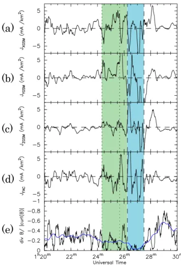
Figure 5 shows the MVAB (blue) and four-spacecraft tim-ing analysis (black) vectors normal to the flow boundaries as arrows, and the flow boundaries themselves as lines in the X-Y, X-Z and Y-Z planes at 01:24:25, 01:25:32, 01:25:47, and 01:26:15 UT (rows a–d, respectively). The green arrows represent the unit vectors of ion velocity perpendicular to the field at those times. The sense of the MVAB and four-spacecraft timing vectors are similar, such that, in each case, the vectors are pointing through the same quadrant. Rows (a) and (d) show a particularly good correspondence between the two analysis techniques, whereas in rows (b) and (c), in which the MVAB vectors had a lower eigenvalue ratio, the correspondence is less good between the two techniques. The vectors in the X-Z plane show that the normals to the boundaries and the motion of the field lines were predom-inantly in the Z direction, although this is expected, given that the plasma sheet field lines are highly distended and contracting. The orientation of the boundary changes in the dusk-dawn direction between rows (a) and (b), representing the boundaries of the first flow burst. This change is not seen between rows (c) and (d), representing the boundaries of the second flow burst, such that both boundaries are orientated towards dusk. We note that at each boundary the ion veloc-ity perpendicular to the field, i.e. the field line motion, was directed more towards dusk than the boundaries in each case. Comparison of the instantaneous magnetic field vector be-tween the four Cluster spacecraft enables the curl and di-vergence of the magnetic field within the tetrahedron to be estimated by the curlometer technique and the net current through the spacecraft tetrahedron to be calculated (Dunlop et al., 1988; Robert et al., 1998, and references therein). We note that the divergence of the magnetic field is zero, from Gauss’ Law, and as such, any measured divergence high-lights the limitations of this analysis technique. We there-fore use the measured divergence as a numerical check by comparing this with the measured curl of the magnetic field. Figure 6 shows the results of the curlometer analysis. Fig-ure 6a–d shows the currents in the X, Y, Z and field parallel (i.e. field-aligned currents) directions deduced from the curl of the magnetic field. Positive field-aligned currents indicate a tailward directed current. The ratio of the divergence of the magnetic field and modulus of the curl of the magnetic field (Fig. 6e) acts as an indication of the quality of the result from the curlometer technique, with lower ratios indicating more reliable results. The analysis output has been smoothed using a 10 s Box Car filter in order to reduce the variability in the data and highlight the large scale structure. The blue line in Fig. 6e is the ratio of the divergence and curl of the magnetic field smoothed with a 60 s Box Car filter to further highlight the lower ratio at the time of the BBF. We note that the un-smoothed currents (not shown) are highly variable, with the polarity of the current changing rapidly. However, such small
(a)
(b)
(c)
(d)
(e)
Fig. 6. Stacked plots of the results of the curlometer analysis of the FGM data from the Cluster spacecraft, showing(a–d)the X, Y, Z and field-aligned components of curl vector of the magnetic field and(e)the ratio of the moduli of the divergence and curl of the magnetic field. The data have been smoothed with a 10 s Box Car filter. The dashed lines represent the zero value in panels (a– d). The blue line (panel e) shows the ratio of the moduli of the divergence and curl of the magnetic field smoothed with a 60 s Box Car filter. The green shaded area indicates the time at which Cluster encountered the BBF and the blue shaded area indicates the low field event. Positive field-aligned currents represent tailward flow, given that Cluster was beneath the current sheet. The dotted vertical lines represent the start of each of the two flow bursts. The dashed vertical lines indicate enclose the low field event.
scale current systems are beyond the scope of this paper, in which we consider the variations in the current on the scale of the flow bursts themselves.
2x10⁵
1x10⁵
0 2x10⁵
1x10⁵
0 2x10⁵
1x10⁵
0 2x10⁵
1x10⁵
0 2x10⁵
1x10⁵
0 (a)
(b)
(c)
(d)
(e)
Fig. 7. The pitch angle distribution of the ion differential num-ber flux for ions with energy>1 keV at(a)01:15:13,(b)01:17:04,
(c)01:21:10,(d)01:24:57,(e)01:28:55 UT. A pitch angle of 180◦ represents Earthward flowing ions.
currents in the plasma sheet can be scaled up, although some-what crudely, using the T96 model magnetic field to give an estimate of the ionospheric field-aligned currents associated with the detected flow of∼18 A km−2. During the low field event (indicated by the blue shading) that follows the BBF, between 01:26:15 and 01:27:45 UT, the field-aligned cur-rents become larger, with peaks>10 mA km−2. The means of the magnitudes of the X, Y and Z components of the mag-netic field and current data show that during this period the Z component of the magnetic field and Y component of the current had the largest components, suggesting that Cluster entered the current sheet. The ratio of the moduli of the di-vergence and curl of the field (Fig. 6e) drops during the pas-sage of the BBF and the low field event, indicating that the results of the curlometer are due to currents flowing through the spacecraft tetrahedron.
Figure 7 shows the pitch angle distribution of ions with energy>1 keV from the CIS instrument on board Cluster 4 at (a) 01:15:13, (b) 01:17:04, (c) 01:21:10, (d) 01:24:57, (e) 01:28:55 UT. These times are indicative of Cluster first en-tering the PSBL, Cluster approaching the inner edge of the PSBL, Cluster located in the plasma sheet before the BBF, Cluster’s encounter with the BBF and Cluster re-entering the plasma sheet, respectively. A pitch angle of 180◦represents Earthward flowing ions. Presented in Fig. 8 is the omni-directional ion differential number flux in the energy range 10 eV to 30 keV between 01:10 and 01:30 UT from the CIS instrument on board Cluster 4. Panel (a) presents the data
i ii
(a)
(b)
01:17:0401:24:57 (a) (b) (c) (d) (e)
Fig. 8. (a)Colour spectrogram of the ion differential number flux for energies in the range 10 eV–30 keV across all pitch angles from the CIS CODIF sensor(b)the ion differential number flux against energy at (black) 01:17:04 and (yellow) 01:24:57 UT. The labels on the bottom axis of panel (a) represent the times of the traces in Fig. 7. Arrows i and ii indicate the times at which Cluster encoun-tered the PSBL and BBF, respectively. The colour scale is shown on the right hand side.
as a spectrogram, whereas panel (b) shows the differential number flux against ion energy at 01:17:04 UT (black) and 01:24:57 UT (yellow). At the bottom of Fig. 8a are letters (a) to (e) representing the times of the pitch angle distributions presented in Fig. 7. From Fig. 8, it can be seen that through-out the interval of interest, the majority of the ion population had energies>1 keV.
(a)
(b)
(c)
i ii
Fig. 9.The differential energy flux of electrons in the energy range 37–2.2×10⁴eV(a)parallel,(b)perpendicular and(c)antiparallel to the magnetic field from the PEACE HEEA sensor on board Cluster 4 between 01:10–01:30 UT shown in colour spectrogram format. The colour scale is shown on the right hand side. The black trace in each panel represents the spacecraft potential in volts. Arrows i and ii indicate the times at which Cluster encountered the PSBL and BBF, respectively. The colour scale is shown on the right hand side.
detected during the BBF encounter. After Cluster encoun-tered the BBF, the spacecraft re-enencoun-tered the plasma sheet, as seen by the isotropic pitch angle distribution (Fig. 7e) and the similarity between the ion differential number fluxes (Fig. 8a).
Presented in Fig. 9 are the differential energy fluxes of electrons moving parallel, perpendicular and antiparallel to the magnetic field (Fig. 9a–c, respectively) from the PEACE HEEA sensor on board Cluster 4 for the interval 01:10– 01:30 UT. The spacecraft potential in volts from the EFW instrument is shown as a black trace at the bottom of each panel. Between 01:10 and 01:18 UT, there is a high flux of low energy (<60 eV) electrons, although comparison with the spacecraft potential shows that these are photo-electrons
-10 -5 0 5 10 15 20
-30 -25 -20 -15 -10 -5 0 (a) 01:15:45
-10 -5 0 5 10 15 20
-30 -25 -20 -15 -10 -5 0
-10 -5 0 5 10 15 20
-30 -25 -20 -15 -10 -5 0
-10 -5 0 5 10 15 20
-30 -25 -20 -15 -10 -5 0 (b) 01:17:48
-10 -5 0 5 10 15 20
-30 -25 -20 -15 -10 -5 0
-10 -5 0 5 10 15 20
-30 -25 -20 -15 -10 -5 0
-10 -5 0 5 10 15 20
-30 -25 -20 -15 -10 -5 0 (c) 01:19:52
-10 -5 0 5 10 15 20
-30 -25 -20 -15 -10 -5 0
-10 -5 0 5 10 15 20
-30 -25 -20 -15 -10 -5 0
-10 -5 0 5 10 15 20
-30 -25 -20 -15 -10 -5 0 (d) 01:21:56
-10 -5 0 5 10 15 20
-30 -25 -20 -15 -10 -5 0
-10 -5 0 5 10 15 20
-30 -25 -20 -15 -10 -5 0
-10 -5 0 5 10 15 20
-30 -25 -20 -15 -10 -5 0 (e) 01:23:59
-10 -5 0 5 10 15 20
-30 -25 -20 -15 -10 -5 0
-10 -5 0 5 10 15 20
-30 -25 -20 -15 -10 -5 0
-10 -5 0 5 10 15 20
-30 -25 -20 -15 -10 -5 0 (f) 01:26:03
-10 -5 0 5 10 15 20
-30 -25 -20 -15 -10 -5 0
-10 -5 0 5 10 15 20
-30 -25 -20 -15 -10 -5 0
-10 -5 0 5 10 15 20
-30 -25 -20 -15 -10 -5 0 (g) 01:28:06
-10 -5 0 5 10 15 20
-30 -25 -20 -15 -10 -5 0
-10 -5 0 5 10 15 20
-30 -25 -20 -15 -10 -5 0
-10 -5 0 5 10 15 20
-30 -25 -20 -15 -10 -5 0 (h) 01:30:10
-10 -5 0 5 10 15 20
-30 -25 -20 -15 -10 -5 0
-10 -5 0 5 10 15 20
-30 -25 -20 -15 -10 -5 0
-10 -5 0 5 10 15 20
-30 -25 -20 -15 -10 -5 0 (i) 01:32:13
-10 -5 0 5 10 15 20
-30 -25 -20 -15 -10 -5 0
-10 -5 0 5 10 15 20
-30 -25 -20 -15 -10 -5 0
-10 -5 0 5 10 15 20
-30 -25 -20 -15 -10 -5 0 (j) 01:34:17
-10 -5 0 5 10 15 20
-30 -25 -20 -15 -10 -5 0
-10 -5 0 5 10 15 20
-30 -25 -20 -15 -10 -5 0
-10 -5 0 5 10 15 20
-30 -25 -20 -15 -10 -5 0 (k) 01:36:21
-10 -5 0 5 10 15 20
-30 -25 -20 -15 -10 -5 0
-10 -5 0 5 10 15 20
-30 -25 -20 -15 -10 -5 0
-10 -5 0 5 10 15 20
-30 -25 -20 -15 -10 -5 0 (L) 01:15:45 <30000 3250 3500 3750 4000 4250 4500 4750 5000 5250 5500 5750 Rayleighs BAS/NIPR DMI
Fig. 10. Eleven consecutive auroral images from the FUV-WIC instrument on board the IMAGE spacecraft, taken from 01:15 to 01:37 UT mapped into the AACGM coordinate system and plotted in MLT-invariant latitude coordinates. The top of each panel rep-resents the 06:00–18:00 MLT meridian. The vertical dotted line in each panel represents the 00:00 MLT meridian. The colour scale of the images is shown on the right hand side. Panel (L) shows the locations of the (green dots) BAS and NIPR LPM magnetometer chain in the Southern Hemisphere and the (blue dots) DMI magne-tometer chain in the Northern Hemisphere in AACGM coordinates and plotted in MLT-invariant latitude coordinates at 01:15:45 UT. The footprint of the Cluster spacecraft in the Southern Hemisphere at that time is shown as a red star in panel (L).
and not part of the natural plasma population. Between 01:24 and 01:26 UT (Fig. 9 arrow ii) the perpendicular electron flux decreased and the electron flux increased in the parallel and antiparallel directions, indicating that Cluster encountered field-aligned beams of electrons, which we interpret as the signature of newly reconnected field-lines (e.g. Keiling et al., 2006), complementing the ion data. We note, however, that the differential energy flux and energy of the electrons was lower during the PSBL crossing compared with the BBF en-counter.
3.2 IMAGE FUV-WIC observations
22:00 23:00 00:00 01:00 02:00 Magnetic Local Time
-12-4
-2
0
2
-4 -2 0 2
Normalised luminosity
1:19:52
1:21:56
1:23:59
1:26:03
UT
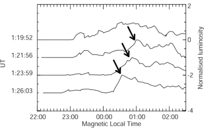
Fig. 11. Time series of normalised auroral luminosity above 3 kR between 01:19 and 01:27 UT. Each trace has been normalised to the maximum luminosity along the trace. The traces plot these values between magnetic latitudes of−67◦and−68◦in the range 22:00– 02:00 MLT. Each successive trace is offset by−1. The arrows in-dicate the signature of the auroral streamer.
01:37 UT. The images have been mapped into AACGM co-ordinates and plotted in MLT-invariant latitude coco-ordinates based on spacecraft pointing data. The dotted rings repre-sent −80◦, −70◦, and−60◦ of invariant latitude from the top of the image outwards. The radial dotted lines represent hours of MLT. The top of each panel represents the 06:00– 18:00 MLT meridian and the vertical dotted lines represent the 00:00 MLT meridian. The T96 model, applied using data from the ACE spacecraft lagged by 44 min, with an error of ±3 min, using the technique of Khan and Cowley (1999), puts the mapped footpoint of Cluster 4 at ∼01:00 MLT throughout the interval. Figure 10L shows the location of the BAS and NIPR LPM magnetometer chains in the South-ern Hemisphere (green dots) and the DMI magnetometers in the Northern Hemisphere (blue dots) in MLT-invariant lati-tude coordinates from AACGM coordinates at 01:15:45 UT. The Cluster footpoint in the Southern Hemisphere is shown as a red star. We note that mapping field lines between hemi-spheres is non-trivial and that equivalent MLT-invariant lat-itude coordinates may not indicate true magnetic conjugacy (see e.g. Østgaard et al., 2004). The FUV-WIC data have been calibrated such that the flat-field and dayglow have been removed. Comparing Fig. 10a and Fig. 10b shows that there was a brightening of the auroral bulge between the images at 01:15:45 and 01:17:48 UT centred at∼01:00 MLT which extended over 2 h of MLT towards dusk and dawn. This indi-cates the start of an auroral substorm expansion phase, which occurred∼1–3 min after Cluster detected the substorm ex-pansion phase in the tail. Figure 10c–k shows that the au-roral bulge expanded polewards, as expected for an auau-roral substorm, to cover∼15◦ of magnetic latitude at its widest point at 01:36 UT. Figure 10 panels (c–k) also show that the auroral breakup was predominantly in the post-midnight
sec-tor. Although the breakup was over the NIPR LPM magne-tometers (around 01:00 MLT, Fig. 10a), the breakup did not expand duskwards to encompass the BAS LPM magnetome-ters until 01:26:03 UT (Fig. 10f). An auroral streamer was evident dawnward of the Cluster 4 footpoint in the images between 01:21–01:27 UT (Fig. 10d–f), highlighted by white circle), giving it a lifetime of 6-10 min, based on the cadence of the FUV-WIC instrument.
Presented in Fig. 11 is a time series of auroral luminos-ity above 3 kR from FUV-WIC taken between magnetic lati-tudes of−67◦and−68◦and between 22:00 and 02:00 MLT from 01:19 to 01:27 UT. The luminosity in each image has been normalised to the maximum luminosity along the trace, such that the maximum data value is 1. The auroral streamer that was detected at 01:21 UT is evident as a peak in the 00:00–01:00 MLT range between 01:21 and 01:26 UT, indi-cated by the arrows on Fig. 11. Successive traces show that this peak moves westwards with a velocity of ∼3 km s−1. Amm et al. (1999) and Sergeev et al. (2004) showed that the bright, duskward edge of an auroral streamer is associ-ated with a large, upward current whereas the trailing diffuse aurora is associated with a smaller downward current. Al-though the peak of the streamer is evident in Fig. 11, the edge of the diffuse aurora is not well defined. As such, we cannot estimate the width of the streamer, and therefore the width of the BBF, solely from the auroral data.
3.3 Ground-based magnetometer observations
20 nT
-20 nT
Fig. 12.Stacked plots of the northward (H) component of the mag-netic field from the west coast magnetometer chain of the DMI Greenland magnetometer network. The dotted horizontal lines rep-resent the baseline (0 nT) for each station. The stations are plotted in descending latitudinal order and the stations corrected geomag-netic latitudes are shown on the right hand side of the plot. Each plot baseline is separated by 250 nT. The vertical dotted lines indi-cate hours. The lower panel shows the northward (H) component of the magnetic field from NAQ filtered using a 4 min high pass filter.
(discounting M79-336) of∼180 s, caused by instrumental ef-fects.
Figure 14 shows stacked plots of the (a) eastward, and (b) vertically downward magnetic field components detected by the NIPR LPM chain between 01:15 UT and 01:35 UT. The vertical dashed line represents the time at which FUV-WIC observed the auroral streamer over the NIPR LPM chain. The eastward component (Fig. 14a) shows a “sawtooth-like” sig-nature accompanied by a minimum in the vertically down-ward (Fig. 14b) component, considered to be a characteristic signature of the streamer (Amm et al., 1999), at the time of the passage of the streamer. This indicates the passage of a weaker east-west current system, in which the current direc-tion changed in the vertical direcdirec-tion during the passage of the structure. However, it should be noted that although the signature is observed at the three stations, timing uncertain-ties in the data of the order of 100 s for both M70-039 and M68-041 mean that the data cannot be used to determine the motion, if any, of the magnetic structure. The timing uncer-tainties in the data from M69-041 were<1 s.
0000 0030 0100 0130 0200 0230 0300
CGM lat.
-77.64
-75.45
-73.31
-72.09
-71.12
-69.14
-68.61
-68.51
-66.32
-65.20
-63.49 Station
code
M85-096
M87-068
M87-028
M88-316
M85-002
M84-336
M82-003
M83-348
M81-338
M79-336
M78-337
500 nT between base lines
LPM Stackplot, H
Fig. 13.Stacked plots of the northward (H) component of the mag-netic field detected by the BAS LPM chain. The dotted horizontal lines represent the baseline (0 nT) for each station. The stations are plotted in ascending latitudinal order and the stations corrected ge-omagnetic latitudes are shown on the right hand side of the plot. Each plot baseline is separated by 500 nT. The vertical dotted lines indicate hours.
4 Discussion
Previous studies of the ionospheric current systems associ-ated with the passage of auroral streamers or BBFs have in-vestigated the currents during various phases of substorm activity. Amm et al. (1999) investigated the current sys-tems associated with an auroral streamer detected 14 min af-ter an auroral breakup and found currents of ∼25 A km−2. Grocott et al. (2004), Sergeev et al. (2004), and Naka-mura et al. (2005) investigated the current systems associ-ated with BBFs during fairly quiet periods (potentially sub-storm growth phases) and found currents ranging from 0.2 to 7 A km−2. The range of these current values (two orders of magnitude) suggests that substorm phase is important to the currents associated with a BBF.
0115 0120 0125 0130 0135
0115 0120 0125 0130 0135
0115
0125
0135 M70-039
M69-041
M68-041
200 nT between base lines
D component
Z component M70-039
M69-041
M68-041
-69.67
-69.29
-68.57
-69.67
-69.29
-68.57 CGM lat. Station
Code
(a)
(b)
Fig. 14. Stacked plots of the(a)eastward (D) and(b) vertically downward (Z) components of the magnetic field detected by the NIPR LPM chain. The dotted horizontal lines represent the base-line (0 nT) for each station. The stations are plotted in ascending latitudinal order and the stations corrected geomagnetic latitudes are shown on the right hand side of the plot. Each plot baseline is separated by 200 nT. The vertical dashed line indicates when the au-roral streamer was above the magnetometer stations, as determined by the FUV-WIC data.
substorm expansion phase onset occurred around 01:15 UT, indicated by an auroral breakup, the formation of an east-west current system accompanied by Pi2 band noise, and a large drop in the tail magnetic field. However, Southern Hemisphere magnetometer data from the BAS LPM chain indicates that an electrojet didn’t form in the Southern Hemi-sphere until 01:25 UT. The timing discrepancy between the Greenland and BAS magnetometers is explained by estimat-ing the position of the auroral breakup region in the North-ern Hemisphere. Østgaard et al. (2004) empirically showed that the offset in location of auroral activity between hemi-spheres is related to the solar wind conditions. Using their results, we estimate that the Greenland magnetometers were near the centre of the breakup region, whereas Fig. 10f shows the auroral breakup region was not over the BAS chain un-til 01:26 UT. We note that the timing discrepancy between the formation of the electrojets in the northern and southern hemispheres (∼600 s) is much larger than the timing error in the BAS LPM data (∼180 s).
As discussed previously, the magnetic field magnitude data from Cluster indicates that the BBF encountered con-sisted of two flow bursts or “bubbles” as described in the model of Chen and Wolf (1993). During the BBF encounter, theBXcomponent of the magnetic field remained negative,
although the gradient of theBY component of the field varied
from negative to positive twice during the encounter. From Sergeev et al. (1996), this indicates that the spacecraft twice
X Y
JFAC
Earth
Fig. 15. Diagram illustrating the relative motion of the Cluster spacecraft across the BBF, looking down on the BBF in the X-Y (GSM coordinates) plane from the current sheet (i.e. into the southern magnetosphere). The BBF consists of two flow bursts. Field-aligned currents associated with the BBF are shown as yellow (Earthward) and grey (tailward) arrows. In both flow burst encoun-ters, the Cluster spacecraft entered the flow burst on the duskward side, close to the nose of the flow, then traversed through to the dawnwards side of the flow burst. The graph indicates the field-aligned currents detected by the spacecraft during their encounter with the each flow burst.
model of Chen and Wolf (1993) as shown by Sergeev et al. (1996). We note that the various analysis methods used show that the flow bursts had significant velocity in the Z direction and that the orientation of the normals to flow boundaries were consistently towards the middle of the plasma sheet. This is consistent with highly stretched magnetic flux tubes convecting and contracting through the plasma sheet.
Data from the NIPR LPM chain showed magnetic signa-tures of auroral streamers, similar to, but weaker than, those reported by Amm et al. (1999). The observations of these signatures were centred at 01:24 UT and with a duration of ∼6–8 min. The magnetic field detected by these magnetome-ters before and during the substorm was highly variable, al-though by comparing the magnetometer and auroral data the magnetic signatures seen around 01:24 UT can be attributed to the BBF. Using the Tsyganenko T96 model and the veloc-ity of the streamer determined from the auroral data this gives the BBF a width of∼3–4RE. This agrees with the expected
dawn-dusk spatial size of a BBF of 3–5RE (Angelopoulos
et al., 1997; Kauristie et al., 2000; Nakamura et al., 2001b). Integrating the ion velocity perpendicular to the field from Cluster 4 during the BBF encounter, and considering that Cluster is essentially stationary during that period (veloc-ity of the order of 1 km s−1 since the spacecraft were near apogee), gives the size of the BBF as 2.3RE.
The event studied by Amm et al. (1999) had background conditions most similar to the event presented here (multiple substorms and streamer detected after an auroral breakup) and, correspondingly, showed very similar field-aligned ionospheric currents (25 A km−2compared with 18 A km−2 detected in our event). The ground magnetic field data pre-sented by Amm et al. (1999) shows a far stronger eastward component signature associated with the passage of the au-roral streamer for a comparatively small change in current.
The event studied by Grocott et al. (2004) occurred during a relatively quiet time, with no apparent substorm activity and was associated with ionospheric currents of ∼0.2 A km−2. The authors compared their ionospheric data with data from FUV-WIC and found that their current sys-tem coincided with an auroral enhancement which had a brightness approximately an order of magnitude lower than the brightness of the streamer presented here. Cowley and Bunce (2001) showed that, based on the theory of Knight (1973) and Lundin and Sandahl (1978), the energy flux into the ionosphere due to aligned currents driven by a field-parallel voltage, such as those that cause the aurora, is related to the square of the field-aligned current. Assuming that, at the energies involved in the currents under discussion, the auroral luminosity is directly related to the energy flux of the electrons, we therefore find that the results of Grocott et al. (2004) are qualitatively consistent with the results presented here.
The field reversals in theBX andBZ directions suggests
that after the passage of the BBF, Cluster crossed a current sheet. This is in agreement with the currents determined
by the curlometer method (Fig. 6), which shows strong cur-rents detected in the X-Y plane. Comparison of the mag-netic fields across the four Cluster spacecraft shows that the magnetic signature was “nested” such that the current sheet moved across the spacecraft then returned, or that the space-craft encountered a convecting feature into which they pen-etrated to differing depths. The magnetic field components during the encounter with this current sheet were not suffi-ciently ordered to allow for meaningful determination of the direction of the motion of the current sheet. Sergeev et al. (1996) showed that the model of Chen and Wolf (1993) pre-dicted that flux tubes in front of a plasma bubble would be displaced by its passage. Sergeev et al. (1996) considered the case of a bubble where the normal to the edge of the bub-ble was in the X-Y plane to demonstrate that there would be a front-side shear. It is, therefore, conceivable that if the bubble was tilted about the X-axis, such that the normal to its edge on the duskward and dawnward flanks had some Z component, that plasma would be displaced in the Z direc-tion also. After the bubble’s passage, the displaced plasma would recoil back towards its original position since the bub-ble causes no persistent dipolarisation of the field, as shown by Lyons et al. (1999). If the current sheet is displaced by this travelling feature and recoils after its passage, the current sheet may overshoot its former position. This could explain why Cluster briefly detects the current sheet.
The origins of BBFs are not yet understood, although they have often been associated with reconnection processes (e.g. Chen and Wolf, 1993; Birn et al., 1999; Sitnov et al., 2005). Based on the simple model of plasma sheet acceleration, as discussed in Cowley (1984), we consider methods of BBF creation by reconnection. We assume the magnetosphere is under-going Dungey Cycle convection (Dungey, 1961) such that there is a reconnection X-line in the far tail. We also as-sume that substorm expansion phase conditions are created by the reconnection of open magnetic flux in the tail by a near-Earth neutral line (NENL) reconnection X-line (Baker et al., 1996, and references therein). In this simple model, the rate of reconnection (EY), theBZcomponent of the
mag-netic field across the current sheet and the velocity of the re-connected field lines (de Hoffmann-Teller velocity,VH T, de
Hoffmann and Teller (1950)) are related by
EY =BZ.VH T (1)
where, for stress balance,VH T is equal to the Alfv´en speed of
the lobe plasma at the reconnection site less the speed of the lobe plasma at the reconnection site. Plasma flows into the reconnection site at theE×Bvelocity from both the northern
and southern lobes and flows out at the velocity of the Earth-ward (VBE) and tailward (VBT) beams, found by coordinate
transformation to be
VBE=2VA−VL≡VH T +VA (2)
whereVA is the Alfv´en speed of the lobe plasma andVLis
nL`
XGSM
(a)
(b)
(c)
(d)
(e)
(f)
D
D S
S
S B
B
(g)
B
Fig. 16.A series of diagrams depicting the generation of a BBF by open field line reconnection. The colours represent field lines with different ion densities. Tailward pointing arrows indicate the motion of the X-lines and Earthward pointing arrows indicate the motion of the reconnected field lines. Panel(a)shows a simple variation of the plasma density in the lobes based on Cowley (1984). Initially the plasma sheet is thin and being populated by the Dungey cycle recon-nection X-line (panelb), with Cluster (represented by the triangle) in the lobe. A substorm X-line forms Earthwards of the Dungey cycle X-line and reconnects through the closed field lines, forming a plasmoid between itself and the Dungey cycle X-line. When the substorm X-line begins to reconnect lobe field lines, the plasmoid is disconnected from the Earth and the plasmoid and substorm X-line retreat tailward. The plasma sheet then expands and the Clus-ter spacecraft are engulfed by the PSBL populated by the substorm X-line (panelc). As the substorm X-line retreats further downtail and the plasma sheet continues to expand, the Cluster spacecraft are engulfed by the central plasma sheet (paneld). A new X-line, lo-calised in the Y direction, forms Earthward of the substorm X-line. This reconnects through the closed field lines, creating a plasmoid between itself and the substorm X-line, and begins to reconnect lobe field lines. This injects lower density lobe plasma into the plasma sheet and creates a BBF (yellow) (panele). The injected plasma then convects through the plasma sheet as a BBF (panelsfandg).
increased ion velocity and BZ component then it is
appar-ent, from Eqs. (1) and (2), that the creation of BBFs requires an increased rate of reconnection (assumingVA is fixed for
a given location in the lobe under the timescales being con-sidered). BBFs can show a decreased plasma density (e.g. Lyons et al., 1999; Nakamura et al., 2005), as in the case presented here. From the model of Cowley (1984), it can be shown that plasma density on the newly reconnected field lines is equal to the density in the lobe source region. As such, in order to create a low density fast flow, the den-sity of the lobe plasma at the source of the flow must be lower than that of the surrounding compressed central plasma sheet. One possibility is that density perturbations within the lobe plasma are coupled with an increased rate of reconnec-tion at the tail X-line, although the mechanisms for creating the density perturbations in the lobes that would necessarily also cause an increase in the reconnection rate upon the field-line reaching the plasma sheet are unclear. Another possibil-ity is that a burst of reconnection occurs closer to the Earth than the global X-line or alternatively, a part of the X-line, localised in the Y direction, moves Earthward. Since lobe plasma density increases with increasing tailward distance, the site of the bursty reconnection would create a low den-sity injection into the plasma sheet if the X-line reconnects through to the open field-lines of the lobe. The reconnected field-lines associated with the low density injection, i.e. the BBF, will necessarily have a higher de Hoffmann-Teller ve-locity than those reconnected at the substorm X-line since, as noted above, the de Hoffmann-Teller velocity is equal to the Alfv´en speed of the lobe plasma being reconnected and Alfv´en velocity is inversely proportional to the plasma den-sity. As such, the BBF will convect through the plasma sheet. What is unclear, from the data presented, is the evolution of the BBF X-line. CIS instrument data shows that the ion den-sity and velocity returns to pre-BBF values over∼1.5 min after the velocity in the X direction reaches its maximum. However, analysis of the flow boundaries indicates that Clus-ter does not pass along the whole length of the flow, rather it exits through the side, such that Cluster does not observe the full evolution of the flow.
rate of reconnection at this new X-line is higher than that of the substorm X-line, such that the X-line reconnects through the closed field lines and eventually reconnects the open field lines of the lobes. This X-line injects plasma from the lobes Earthwards of the substorm line (Fig. 16e), such that the ion density on these field lines is lower than the surrounding field lines. Since the Alfv´en speed of the plasma is inversely re-lated to the plasma density, the speed of the field lines away from the reconnection site is higher, hence the field lines con-vect through the plasma sheet as a BBF. As noted above, the data presented are insufficient to determine the full evolution of the new X-line. For illustrative purposes, we show the BBF as a convecting bundle of flux that is no longer being fed by the line that created it (Fig. 16f and g), with the X-line retreating downtail in a manner similar to the substorm recovery phase (e.g. Hones, 1984).
The above model considers the origins of a BBF to be re-connection of open field lines. This agrees with the work of Lyons et al. (1999) and Grocott et al. (2004) who associated BBFs with pseudo-breakups, which are often considered to be the localised closure of open flux. If we consider sub-storm reconnection to take place at a single X-line, as in the NENL and current disruption models, and the creation of a BBF to occur Earthwards of that line then such a burst of reconnection would create a flux rope Earthwards of the sub-storm reconnection site as shown in Fig. 16e. The subsub-storm X-line creates a flux rope between itself and the downtail (Dungey cycle) X-line, hence there would be two flux ropes in the tail. It has been suggested that the passage of multi-ple flux ropes is a signature of multimulti-ple X-line reconnection (e.g. Slavin et al., 2005), hence the detection of BBFs during substorms could also be considered to be a signature of mul-tiple X-lines. Alternatively, the generation of a BBF could be considered to show that substorm reconnection does not occur on one “global” X-line, but on a series of X-lines sep-arated in the Y direction, such as has been suggested for flux transfer events at the dayside magnetopause. A BBF could be generated by an X-line markedly Earthwards of the av-erage position of the substorm X-lines. The model is also applicable to “quiet” time observations of BBFs. It is gen-erally accepted that Dungey Cycle reconnection in the tail is ongoing. As such, any reconnection Earthwards of the Dungey Cycle X-line would inject low density plasma into the plasma sheet. A recent study by Grocott et al. (2007) has provided evidence of localised tail reconnection during quiet times, termed by the authors as tail reconnection during IMF northward non-substorm intervals, or TRINNI, and the de-tection of an associated BBF, hence reconnection is a viable method by which to inject BBFs into the plasma sheet dur-ing both quiet and disturbed times. It should be noted that this model does not consider the evolution of the motion of the BBF through the substorm populated plasma sheet and is complementary to the model of Chen and Wolf (1993), who only considered the time evolution of a plasma bubble after its generation and not the generation mechanism itself.
Particle data from the CIS and PEACE instruments dur-ing the BBF are consistent with the above reconnection model. During reconnection, both ions and electrons are en-ergised in the field-aligned direction. The velocity of the electrons away from the reconnection is greater than that of the ions, hence electrons will mirror in the inner mag-netosphere and return along the field lines before the ions such that bidirectional electron beams form before bidirec-tional ion beams. During this event, bidirecbidirec-tional ion and electron beams are observed by Cluster when it passes into the PSBL at 01:15 UT (Fig. 7a and b and Fig. 9). During the encounter with the BBF at 01:24 UT, Cluster observed a bidirectional electron and ion beams, although the Earthward ion beam had a greater differential number flux than the tail-ward beam (Figs. 7c and 9), suggesting that the spacecraft were sufficiently close to the reconnection site that the ma-jority of the ion population had insufficient time to mirror in the inner magnetosphere and return to the spacecraft po-sition, such that the BBF consisted of recently reconnected field lines. Cluster detected a dispersed ion energy signature when the spacecraft crossed the PSBL (Fig. 8a), indicating that the PSBL was the result of reconnection. During the BBF encounter, the ions were energised to a level similar to that in the PSBL, although there was no apparent energy dis-persion. Given that estimates of the width of the BBF from ground-based data and from integrating the ion velocity per-pendicular to the magnetic field during the BBF encounter are∼3RE and BBFs are considered to be long and narrow
(Sergeev et al., 2000; Amm and Kauristie, 2002), and that the spacecraft crossed the width of the BBF, it is conceiv-able that the spacecraft did not travel far enough along the BBF to detect any energy dispersion. The similarity between the ion density during the passage of the BBF and the earlier PSBL crossing (Fig. 3a) suggests that the BBF reconnection site was close to the location of the substorm X-line location when Cluster was engulfed by the PSBL.
5 Conclusions
the duskward and exited on the dawnward side. The pro-jected ionospheric field-aligned currents were found to be ∼18 A km−2, comparable to the measured ionospheric cur-rents associated with an auroral streamer as reported by Amm et al. (1999), who also obtained their readings during a period of multiple substorms and after an auroral breakup. The detection of currents that, when projected into the iono-sphere, are comparable with the currents detected in associ-ation with auroral streamers lends support to the argument that auroral streamers can be considered the auroral manifes-tation of BBFs.
The results presented are consistent with a model of the connection of open field-lines Earthward of the substorm re-connection region for BBF generation based upon the plasma sheet acceleration model of Cowley (1984). The pitch an-gle distribution of the ions from the CIS instrument on Clus-ter 4 showed that during the passage of the BBF the ions were approximately field-aligned in an Earthwards direction, whereas the electrons showed bi-directional beams, indicat-ing that Cluster encountered recently reconnected field lines. The elevatedBZ component indicates that the reconnection
event that generated the BBF had a greater rate of reconnec-tion than the source of the plasma sheet detected around the flow. Since the lobe plasma density increases with distance from the Earth, reconnection of open (lobe) field lines closer to the Earth than the substorm X-line would inject lower den-sity plasma into the plasma sheet. This is also consistent with the notion that pseudo-breakups are BBFs outside of substorm times.
Acknowledgements. The authors wish to thank CDAWeb for
pro-viding the IMAGE FUV-WIC data; ESA Cluster Active Archive for providing the full resolution FGM data; M. P. Freeman, M. Rose and others at the British Antarctic Survey for providing the low power magnetometer data. Thanks go to the operations teams of the various instruments used in this study. Analysis of the Cluster FGM data and CIS moments was done with the QSAS science anal-ysis system provided by the United Kingdom Cluster Science Cen-tre (Imperial College London and Queen Mary, University of Lon-don) supported by PPARC. M. Lester, R. C. Fear, A. Grocott, and S. E. Milan were supported by PPARC grant PPA/G/O/2003/00013 and STFC grant PP/E000983. During this study C. Forsyth was supported by STFC studentship PPA/S/S/2005/04156, while S. W. H. Cowley was supported by a Royal Society Leverhulme Trust Senior Research Fellowship.
Topical Editor I. A. Daglis thanks O. Amm and another anony-mous referee for their help in evaluating this paper.
References
Amm, O.: Direct determination of the local ionospheric Hall con-ductance distribution from two-dimensional electric and mag-netic field data: Application of the method using models of typi-cal ionospheric electrodynamic situations, J. Geophys. Res., 100, 21 473–21 488, doi:10.1029/95JA02213, 1995.
Amm, O.: Method of characteristics in spherical geometry applied to a Harang-discontinuity situation, Ann. Geophys., 16, 413–
424, 1998,
http://www.ann-geophys.net/16/413/1998/.
Amm, O. and Kauristie, K.: Ionospheric signatures of bursty bulk flows, Surv. Geophy., 23, 1–32, 2002.
Amm, O. and Viljanen, A.: Ionospheric disturbance magnetic field continuation from the ground to the ionosphere using spherical elementary current systems, Earth, Planets, and Space, 51, 431– 440, 1999.
Amm, O., Pajunp¨a¨a, A., and Brandstr¨om, U.: Spatial distribution of conductances and currents associated with a north-south auro-ral form during a multiple-substorm period, Ann. Geophys., 17, 1385–1396, 1999,
http://www.ann-geophys.net/17/1385/1999/.
Angelopoulos, V., Baumjohann, W., Kennel, C. F., Coronti, F. V., Kivelson, M. G., Pellat, R., Walker, R. J., Luehr, H., and Paschmann, G.: Bursty bulk flows in the inner central plasma sheet, J. Geophys. Res., 97, 4027–4039, 1992.
Angelopoulos, V., Kennel, C. F., Coroniti, F. V., Pellat, R., Kivel-son, M. G., Walker, R. J., Russell, C. T., Baumjohann, W., Feld-man, W. C., and Gosling, J. T.: Statistical characteristics of bursty bulk flow events, J. Geophys. Res., 99, 21 257–21 280, 1994.
Angelopoulos, V., Phan, T. D., Larson, D. E., Mozer, F. S., Lin, R. P., Tsuruda, K., Hayakawa, H., Mukai, T., Kokubun, S., Ya-mamoto, T., Williams, D. J., McEntire, R. W., Lepping, R. P., Parks, G. K., Brittnacher, M., Germany, G., Spann, J., Singer, H. J., and Yumoto, K.: Magnetotail flow bursts: association to global magnetospheric circulation, relationship to ionospheric activity and direct evidence for localization, Geophys. Res. Lett., 24, 2271–2274, doi:10.1029/97GL02355, 1997.
Baker, D. N., Pulkkinen, T. I., Angelopoulos, V., Baumjohann, W., and McPherron, R. L.: Neutral line model of substorms: Past results and present view, J. Geophys. Res., 101, 12 975–13 010, doi:10.1029/95JA03753, 1996.
Baker, K. B. and Wing, S.: A new magnetic coordinate system for conjugate studies at high latitudes, J. Geophys. Res., 94, 9139– 9143, 1989.
Balogh, A., Carr, C. M., Acu˜na, M. H., Dunlop, M. W., Beek, T. J., Brown, P., Fornac¸on, K.-H., Georgescu, E., Glassmeier, K.-H., Harris, J., Musmann, G., Oddy, T., and Schwingenschuh, K.: The Cluster Magnetic Field Investigation: Overview of in-flight performance and initial results, Ann. Geophys., 19, 1207–1217, 2001,
http://www.ann-geophys.net/19/1207/2001/.
Birn, J. and Hesse, M.: Details of current disruption and diversion in simulations of magnetotail dynamics, J. Geophys. Res., 101, 15 345–15 358, doi:10.1029/96JA00887, 1996.
Birn, J., Hesse, M., Haerendel, G., Baumjohann, W., and Shiokawa, K.: Flow braking and the substorm current wedge, J. Geophys. Res., 104, 19 895–19 904, doi:10.1029/1999JA900173, 1999. Birn, J., Raeder, J., Wang, Y., Wolf, R., and Hesse, M.: On the
propagation of bubbles in the geomagnetic tail, Ann. Geophys., 22, 1773–1786, 2004,
http://www.ann-geophys.net/22/1773/2004/.