A Work Project presented as part of the requirements for the Award of a Masters Degree in Economics from the NOVA – School of Business and Economics
Cost Efficiency in the Portuguese
Water Sector
The case of multimunicipal systems operating at the
bulk level
Tiago Lopes da Silva
Student number 520
A Project carried out on the Applied Policy Analysis major, under the
supervision of Professor Susana Peralta
-1-Abstract: The purpose of this paper is to study the cost efficiency of multimunicipal systems operating at the bulk level in the Portuguese water sector. We will use Pooled OLS, Fixed Effects and Stochastic Frontier Analysis (SFA) to study the role of structural variables such as water losses, network density, water sources, quality measures, rainfall and topography in explaining the cost differences among those systems. Moreover, using SFA we determine
operators’ efficiency scores. We found that inefficiency of operators remained constant over time. The main source of the distance to the cost frontier is a high degree of inefficiency and not exogenous random shocks.
Keywords: Portuguese water sector; wholesale market; cost efficiency; Stochastic Frontier Analysis (SFA).
Acknowledgments: I would like to express my gratitude to Professor Susana Peralta for her
inspiring orientation and everlasting patience. I also express my acknowledgment to the Department of Financial and Economic Analysis (DEF) of the Water and Waste Services Regulation Authority (ERSAR), particularly in the person of Luís Pereira for his availability and enthusiasm that supported me throughout the last months. Any remaining errors or ambiguities are exclusively of my own responsibility.
1- Introduction.
-2-single firm minimizes total costs. In addition, water operators usually develop their activities under regional exclusivity. In other words, they can be both legal and natural monopolies. A monopolistic market structure potentially entails three types of inefficiency: allocative, technical and dynamic. Firstly, a monopolist is bound to produce less and charge a higher price for its output when compared to the competitive case, implying allocative inefficiency: some units are not produced for which consumers would be willing to pay more than the social marginal cost of production. Moreover, a monopolist is technically inefficient when it does not necessarily produce the maximum possible output using the minimum quantity of inputs. Additionally, sectors characterized by a lack of competitive pressure tend to present lower rates of innovation, implying potential dynamic inefficiencies.
The absence of a competitive environment in the water sector brings about the need for fair prices and the reduction of losses in social well-being. Therefore, under a normative view, there appears to be public interest justifications for regulatory intervention. In this context, benchmarking becomes very relevant since it helps regulatory authorities to define the appropriate policy instruments for the sector, while inducing the so called “good behavior” and potentially enhancing operators’ productivity.1 Moreover, the improvement in econometric
methods throughout time and the increasing availability of data (i.e. the existence of longer panels) favored the discussion and the growing interest about efficiency analysis.
The aim of this paper is to study the cost efficiency of multimunicipal systems operating at the bulk level in the Portuguese water sector. These systems were created with the purpose of operating bulk activities. The vast majority of studies only considers operators that supply water or provide wastewater services to final users (retail market), excluding operators which act as wholesalers (bulk level).
1 In broad terms, “good behavior” can be interpreted as incentives alignment between the regulatory authority and the regulated
-3-We will use Pooled OLS (POLS), Fixed Effects (FE) and Stochastic Frontier Analysis (SFA) to study the role of structural variables such as water losses, network density, water sources, quality measures, rainfall and topography in explaining the cost differences among those systems. Moreover, using stochastic frontier models for panel data we determine operators’
technical efficiency scores.
The importance of this type of papers relies on the encouragement of more efficient performances. Nevertheless, the existing data constraints and the difficulties in ensuring data comparability implicitly require that the conclusions here presented should be interpreted with some prudence and should never be read in an isolated manner. We must emphasize that the choice of the econometric strategy, the selection of specific variables and the inherent quality of data can potentially be reflected in substantially different empirical results.
The remainder of the text is structured into sections. In Section 2, an overview of the Portuguese water sector is provided. In Section 3, we review some literature regarding cost efficiency in the water sector. In Section 4, we describe the data and the underlying methodology. In Section 5, the empirical results are presented and discussed. Finally, Section 6 concludes the paper.
2- The Portuguese water sector: an overview.
Throughout this text, whenever water sector is mentioned, it is our purpose to encompass two distinct but complementary services within the scope of sanitation: the drinking water supply service (AA) and the wastewater management service (WW). Unlike what happens in most EU members, the Portuguese water sector is not vertically integrated – it is characterized by a bulk-retail dichotomy in the supply chain.
-4-In order to overcome geomorphological barriers, water circulates under pressure in pipes to a given treatment plant. This stage is known as water elevation. In treatment plants, the water characteristics are corrected in such a way that it becomes safe for human consumption. Subsequently, treated water is transported from the zone of production (upstream) to the zone of consumption (downstream), where it is stored to ensure continuity of supply. Since the industry is not vertically integrated, it is then responsibility of the retailers to ensure the water distribution to final consumers. A complementary activity is the management of wastewater. The first stage consists in wastewater collection, which is done by retailers. Following the drainage and elevation, the treatment of wastewater is done by those operating at the bulk level. Moving up in the supply chain, another stage is sludge processing. After this stage, the solid content is transported to an adequate final destination, such as agricultural use or to a landfill, while the liquid content is discharged in the water environment.
In the beginning of the 1990s, it was then considered that Portugal presented very poor indicators regarding population coverage of drinking water supply and basic sanitation: 80% and 60% of coverage, respectively. Almost 20 years later, a significant improvement was registered. According to the most recent statistics, in 2009, 96% of the Portuguese population was served by drinking water supply and 84% already had access to basic sanitation.2
Undeniably, 1993 represents a crucial year in explaining the significant changes that took place in the Portuguese water sector. From 1977 to 1993, the Law of Sectors’ Delimitation (Law no. 46/77, July 8) clearly defined which sectors of the economy were not allowed to belong to the private initiative. The water sector was one of them. In 1993, it became possible to open the sector to private investors. Until then, it was responsibility of the Portuguese municipalities to ensure the reasonable operation of local water supply and wastewater management services.
-5-The only exception was EPAL in the municipality of Lisbon.3 Following the structural changes in the sector, Águas de Portugal was created in 1993, to speed up the development of multimunicipal systems, aimed at correcting the considerable heterogeneity and local fragmentation that characterized the Portuguese water sector. In addition, multimunicipal systems were created to ensure stable and safe drinking water quality, and to enlarge the access to basic sanitation. The Decree-Law no. 379/93 (November 5) then established the division between bulk and retail activities. Finally, it must also be recognized that since Portugal joined the European Economic Community (EEC), in 1986, the access to European funds allowed significant investments in network infrastructures.4
Since 1997, Portugal has its own national regulation authority for the water sector (Decree-Law no. 230/97, August 30). ERSAR (formerly IRAR – Institute for the Regulation of Water and Solid Waste) is the Portuguese water and waste services regulation authority, and also the national authority for drinking water quality control. Initially, its jurisdiction in terms of
economic regulation was limited to concessions and to a “soft” regulatory approach known as
“sunshine regulation” – comparison of performance indicators applied to each operator, followed by their public display. This form of regulation is not coercive and rests on engaging operators in a virtual form of competition: operators are expected to react to that public display of information in such a way they try to improve and achieve a better place in the next year’s ranking. Given these limitations, an effort was made so that its powers and scope of action have
3 The Decree-Law no. 553-A/74 (October 30) created EPAL – Empresa Pública das Águas de Lisboa in substitution of CAL – Companhia das Águas de Lisboa, which was the concessionaire of water supply services to the city of Lisbon between 1868 and 1974. In 1991, it was transformed in a public limited company (Decree-Law no. 230/91, April 21), and renamed to EPAL –
Empresa Portuguesa das Águas Livres, SA.
4 For example, between 1986 and 1988, Portugal received from the European Commission the equivalent to 1185 millions of
-6-been enlarged in the last years. At the time of writing, ERSAR is rethinking its regulatory model and new legislation is under discussion in order to ensure an independent regulation.
3- Literature review.
The existing empirical literature on the water sector comprises the following topics: 1) the debate between public and private ownership; 2) the findings related to economies of scale, economies of output density and economies of scope; 3) the estimation of cost frontiers and efficiency scores; 4) the role of structural variables (e.g. population density, water sources and elevation differences) and the introduction of quality indicators, such as water losses and chemical treatment. In the next lines, a comprehensive literature survey is provided.
Regarding the debate between public and private ownership, the main conclusion to derive from the literature is the existence of very modest empirical justifications for a general conjecture in favor of each type of ownership. When looking for evidence regarding the merits of public versus private ownership in Portugal, again no clear picture emerges. On the one hand, Martins, Fortunato and Coelho (2005) found that private ownership is statistically significant and positively related to total costs. On the other hand, Correia (2008) concluded that private ownership is statistically significant but negatively related to total costs. Although both authors use similar data sources, they use different econometric approaches.5 Moreover, the residuality of private ownership may also explain such opposite conclusions. In light of Walter et al. (2009), the conclusion is that the merits of ownership should not be studied alone, because the institutional context and the regulatory model also play an important role. In this paper, since the Portuguese State is the majority shareholder in multimunicipal systems, the question of ownership will not be our main interest.
5 Martins, Fortunato and Coelho (2005) use a cubic cost function application, while Correia (2008) prefers to follow SFA and
-7-Researchers have been demonstrating a growing interest about efficiency analysis in the water sector. Therefore, it is not difficult to find several studies for the majority of developed countries. Fraquelli and Moiso (2005) studied the cost efficiency and economies of scale in the Italian water sector using a stochastic frontier approach. They found that vertical integration seems to generate economies of scale, implying that the optimum size of operators should be revised. Inefficiency scores are initially increasing and then tend to decrease over time. Zschille and Walter (2011) analyzed the performance of public and private water utilities in Germany and applied both Data Envelopment Analysis (DEA) and SFA. In order to account for structural differences in water supply, they considered explanatory variables such as output density, water losses, ratio of groundwater input, elevation differences, per-capita debt of municipalities, and dummy variables for location in East Germany, governance mode and joint provision of water and sewerage services. Efficiency levels under SFA are considerably higher than those predicted by DEA, which can be explained by methodological differences between these approaches.6 In general, they conclude for the absence of economies of scope between water and sewerage. Moreover, a higher share of water losses, higher output density, higher elevation differences and location in East have a positive and statistically significant impact on costs. On the other hand, the per-capita debt of a municipality and private ownership are not statistically significant. Bottasso and Conti (2003) analyzed the evolution of operating cost inefficiency for the English and Welsh water industry over the 1995-2001 period by estimating an heteroskedastic stochastic variable cost frontier. They found that industry operating cost inefficiency has decreased over the sample period and that inefficiency differentials among firms have steadily narrowed. The authors suggest that their findings rest on efficiency enhancing effects brought about by incentives provided in the context of the 1989’s sector
6 DEA is a non-parametric approach based on linear programming techniques. Comparing to SFA, DEA is very sensitive to
-8-privatization and subsequent changes in the regulatory model in order to introduce yardstick competition. Coelli and Walding (2005) provide the first published set of comprehensive performance measures for the Australian water supply industry. DEA is used to provide measures of technical and scale efficiency for each operator. Their results indicate that the average firm has a technical efficiency score of 90.4%. Another example is the study by Filippini, Hrovatin and Zoric (2007) for the Slovenian water distribution utilities. The levels of efficiency estimates as well as the corresponding rankings strongly depend on the econometric model specification, meaning some volatility in their conclusions. Nevertheless, the different models produce consistent findings regarding economies of density (output and customer) and economies of scale.
The econometric contributions presented in this section should be compared with some prudence. Reliability of data, data comparability issues and different estimation techniques contribute to different conclusions, recommending that performance measures should be interpreted very carefully.
4- Data and methodology.
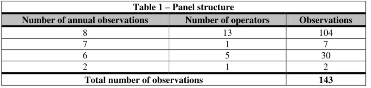
As initially stated, the purpose of this paper is to study the cost efficiency of multimunicipal systems operating at the bulk level in the Portuguese water sector. An unbalanced panel data is used including all operators over the 2004-2011 period, consisting of a total of 143 observations. Not every operator is yearly observed between 2004 and 2011, explaining the panel unbalancedness.7 The dataset used in this paper covers 20 firms, including at most 8 observations per operator and a minimum of 2. The following table characterizes the panel structure:
7 For the following firms data was collected after the panel first year: Águas do Centro Alentejo (2005), Águas do Mondego
(2006) and SIMARSUL (2006). Águas do Noroeste arose in 2010 from the merger of 3 multimunicipal systems: Águas do Ave,
-9-Table 1 – Panel structure
Number of annual observations Number of operators Observations
8 13 104
7 1 7
6 5 30
2 1 2
Total number of observations 143
The data was taken from the Annual Reports on Water and Waste Services in Portugal (RASARP), the regulator’s online private database (Portal ERSAR) and from the operators’
annual financial statements (Relatório e Contas). Based on the Portuguese fiscal year, each year of observation starts at January 1 and ends the following December 31.
As suggested by standard microeconomic theory (Varian, 2010), in order to estimate a cost function we need information on input prices and output quantities. It is also possible to include other explanatory variables to account for the sector specific characteristics. These are often
named “structural variables” or “output characteristic variables”. In our cost model
specification, we consider that operators use 2 inputs (L: labor; K: capital), with the corresponding pricespLandpK. They can produce 2 outputs: water (YAA) and wastewater services (YWW). Billed water was used as YAA and collected wastewater as YWW(both variables
are expressed in thousands of m3). Since there is no specific information on input prices, proxies were used to overcome this problem. In this context, we followed the suggestions of Lin (2005), Fraquelli and Moiso (2005), and Filippini, Hrovatin and Zoric (2007).
-10-can appear in the numerator and denominator. In our model, capital costs only consist of
depreciation expenses, that is, the recognition in costs that asset’s value decrease during the
period in which it is expected to be used. The capital stock is approximated by the annual treatment capacity. This variable is obtained multiplying by 12 the monthly maximum treatment capacity. Since it is expressed in m3 of water, in the case of multi-output operators we just added the water treatment capacity to the wastewater treatment capacity.
The dependent variable, total costs (TC), is obtained by adding up four main components: labor costs, depreciation, costs of goods sold (e.g. water and wastewater treatment products) and external supplies (essentially, energy costs). On average, the cost structure of multimunicipal systems is characterized by 20% of labor costs, 40% of depreciation costs and the remaining 40% corresponds to the cost of goods sold and external supplies. The small values of standard deviations associated to each weight suggest a very low variability of the cost structure among operators, which was expectable since they belong to the same shareholder (Águas de Portugal), implying harmonization of management choices.
To the best of our knowledge, the issue of endogeneity is not acknowledged in the references mentioned in this paper. Nevertheless, we should recognize beforehand that the way input prices are proxied potentially leads to endogenous regressors. In order to overcome this problem we estimated our regressions using input prices lagged 1 period (pLt1andpKt1), implying the loss of 20 observations.
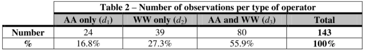
-11-the different types of operators included in -11-the sample, since each type is allowed to have a different intercept or, when considering interactions with other explanatory variables, a different slope. Whenever we were interested in a specific variable for water supply operators, in order to perform an interaction, we defined the dummy d13d1d3. In a similar way, for wastewater management operators: d23 d2d3.
Table 2 – Number of observations per type of operator AA only (d1) WW only (d2) AA and WW (d3) Total
Number 24 39 80 143
% 16.8% 27.3% 55.9% 100%
The network length corresponds to the kilometers of pipes and collection network. This is an
important variable to distinguishing between economies of output density and economies of scale. We expect that more kilometers of network increase total costs of operators. As a proxy
for population density we used the ratio between the number of houses covered by the system
and the size of service area (in km2). We expect an ambiguous effect for this variable. On the one hand, it can be more costly to serve more dispersed consumers, because more network infrastructure is needed per connection. On the other hand, there is the possibility of congestion problems in more densely populated areas. In our cost model, we also recognize the role of
water abstraction sources: surface water, groundwater or both sources. Under the assumption
that surface water abstraction requires more treatment to purify the water, as stated in Bottasso and Conti (2003) and Zschille and Walter (2011), we defined the following dummies to evaluate the impact of water sources on total costs: dSurface1 if the operator only uses surface water and dGroundwater 1 for groundwater abstraction only. Since this is a time-invariant regressor, we will assess its impact on costs under Pooled OLS estimation.
It is also interesting to evaluate the role of water losses in explaining total costs. By water losses
-12-Following the approach of Correia (2008) and Zschille and Walter (2011), we obtained the losses ratio as the ratio between water losses and total water input (m3 of water in the system). As pointed out by Coelli and Walding (2005), the type of soil can influence total costs by means of higher water losses. They argue that clay soils are more prone to pipe breakages, leading to higher maintenance costs. However, considering a longer time horizon, water losses do not only depend on exogenous circumstances. Indeed, water losses allow us to evaluate the status of infrastructures: older networks and lack of maintenance decisively contribute to higher water losses. Therefore, two effects should be considered: higher water losses today may increase total costs today via the reintroduction of water in the system; on the other hand, higher water losses today may also mean higher total costs in the following period via better network maintenance and replacement investments. However, in subsequent periods, a renewed water network will probably reduce the costs of reintroducing water in the system to compensate for losses. Considering the available literature, it is often missing a reference to additional influencing factors such as output quality, climatic conditions or geomorphological characteristics. This
paper will try to assess the impact of those factors in operators’ total costs. Lin (2005) explores the introduction of output quality variablesand their impact on operators’ performance. The
underlying idea is that quality improvements raise costs. In order to study this aspect, we calculated the water quality indicator (WQI) used by ERSAR, which is the percentage of water analyses that met the parametric values. We then converted those values into an ordered scale:
“10” for WQI0.970; “20” if 0.970WQI 0.990; “30” if 0.990WQI0.995; “40”
if 0.995WQI 1.000; and “50” when WQI 1.000. In what concerns climatic influences, we want to study the impact of average rainfall on total costs. Annual climatic bulletins
-13-the operator’s type, we expect different signs for -13-the impact of rainfall on total costs. On -13-the one
hand, lower levels of rainfall reduce the quantity of surface water, forcing the multimunicipal systems to import water from neighboring systems or, alternatively, to explore other sources of groundwater abstraction. On the other hand, in the case of wastewater management services, due to specific network configuration, rain is collected by drains and gullies before being removed by the operator via public sewer. Therefore, when drainage does not separate rain from wastewater, a higher level of rainfall can potentially increase treatment costs. Furthermore,
geomorphological characteristics can also influence operators’ performance. A hilly
topography, that is, considerable elevation differences within the service area of a given
operator will probably require higher pumping costs. In order to assess this aspect, we combined a hypsometric map with a map showing the delimitation of each multimunicipal system and constructed the variable “average elevation” (expressed in meters). This variable was calculated as the average between the highest and the lowest point within the area covered by each system. A higher average elevation is thus expected to increase operators’ costs, regardless of their type. Finally, depending on the model specification, time fixed effects were also included in order to
capture unobserved year effects and to see how total costs have behaved over time.
The estimation of a cost function requires a functional form. In the existing literature, the most common functional forms are the Cobb-Douglas and the transcendental logarithmic (translog) specification. Despite its flexibility, the translog specification often violates the assumptions of monotonicity and concavity, which are desirable for a cost function.8 Moreover, since the interactive terms are usually highly correlated it potentiates multicollinearity problems (one variable can be linearly predicted from the others), thus influencing the model statistical significance. Furthermore, in small samples, too many degrees of freedom are consumed. In
8 A detailed discussion about the desirable properties of a cost function can be found in
-14-light of these reasons, we decided to adopt the Cobb-Douglas specification. In order to obtain linearity in the parameters, we took the natural logarithm of all continuous variables, such that the estimated coefficients can be read as elasticities.9 A general example of a log-linear form of the Cobb-Douglas model is presented below (where Z is a given structural variable and D a possible dummy variable):
In this paper, a more complete version of the cost model presented above is estimated using Pooled OLS, Fixed Effects (FE) and Stochastic Frontier Analysis (SFA). Given the specific characteristics of each estimation approach, the cost model may present different specifications. For example, if we are interested in the role of several time-invariant explanatory variables (e.g. water sources or geomorphological characteristics), the FE model should be disregarded. Therefore, we should use of Pooled OLS or Random Effects (RE). The FE (or “within”) estimator, which explores the variation in data over time, eliminates the fixed effects by mean-differencing and provides consistent estimators for the FE model. We cannot estimate the coefficient on a invariant variable since all observations of the mean-difference of a time-invariant variable are 0. RE is an alternative, but it does not control for unobserved heterogeneity which is constant over time. In this case, the estimators may be biased. Although it yields estimates of all coefficients even those of time-invariant regressors, RE considers unobserved individual heterogeneity as being distributed independently of the regressors. This is a stronger assumption comparing to FE but it is often unsupported by the data.10 If the appropriate model is FE, Pooled OLS and RE both yield inconsistent estimators.
Nevertheless, none of those least squares-based regression techniques is particularly suitable for studying cost efficiency. Indeed, several factors influence the structure of the production process
9 When necessary, in order to allow for linearization, 0 values were replaced by 10-9. 10 For a comprehensive discussion of linear panel models:
Cameron, A. Colin and Pravin K. Trivedi. 2009. Microeconometrics – Methods and Applications, 8th edition, New York: Cambridge University Press, pp. 697-778.
it
it Lit Kit it it it
it it it it K it L it it D Z p p Y TC D Z p p Y TC 5 4 3 2 1 0 5 0 ln ln ln ln exp ln exp exp exp
exp 1 2 3 4 (1)
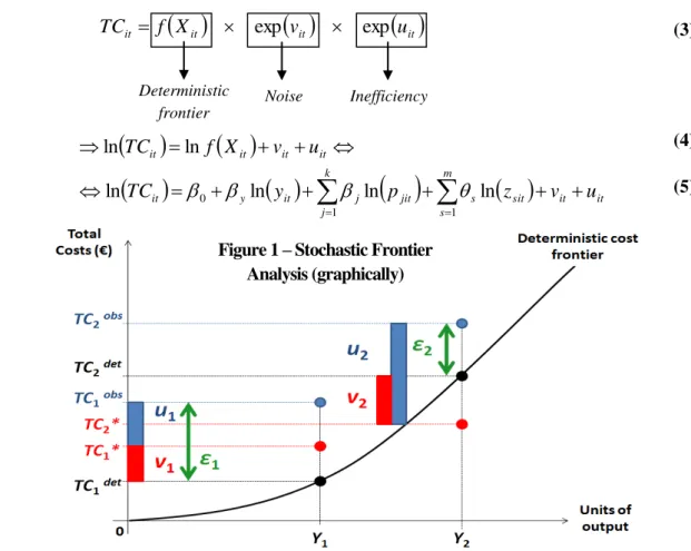
-15-which, in turn, can explain the differences in efficiency behavior among firms. Knowing that, almost always, firms are not successful optimizers, SFA – introduced by Aigner, Lovell and Schimidt (1977) – is an econometric technique that allows modeling this type of behavior. Since it produces efficiency scores, we can obtain information for benchmarking purposes, which might justify its increasing popularity in the literature. The main particularity of SFA is that the error term is divided in two components: uit is a non-negative random variable representing the
operator’s own inefficiency and vit is a noise term, which can be positive or negative, reflecting
the influences affecting the operator (vit 0 if it operates in a favorable environment and 0
it
v if it faces a negative environment). In a panel data context, assuming that there are k
inputs and m structural variables, the cost frontier can be specified as:11
it itm s sit s k j jit j it y it it it it it it it it it u v z p y TC u v X f TC u v X f TC
1 10 ln ln ln
ln ln ln exp exp
11 The graphical example is based on Figure 9.1 (p. 244) from
Coelli et al. 2005. An Introduction to Efficiency and Productivity Analysis, 2nd Edition, Springer, New York.Although Coelli et al. present the case of a production frontier, the cost frontier
model is very similar and easy to derive: instead of production as dependent variable we have total costs, quantities of inputs (K and L) are substituted by input prices as regressors, and the inefficiency termis multiplied by -1.
Deterministic
frontier Noise Inefficiency
Figure 1 – Stochastic Frontier Analysis (graphically)
(3)
-16-Total costs of inefficient firms
uit 0
lie above the minimum established by the cost frontier, that is, obs it*it TC
TC . Obviously, efficient firms operate at the frontier
uit 0
. Therefore, bydefinition, we have: it it
obs
it TC u
TC * ;TCit*TCitdetvit; it it it it
obs
it TC u v
TC det .
Figure 1 illustrates the typical case of 2 firms. On the one hand, firm 1 operates in an unfavorable environment
v1 0
, implying total costs at the frontier higher than the deterministic value
TC TCdet
1
1* . On the other hand, firm 2 faces a favorable operating environment
v2 0
.12 Since v2 u2 2 0, observed total cost for firm 2 is higher than the deterministic value
TC obs TC det
2
2 . Following the notation presented before, we can easily obtain the efficiency score for firm i at time t from the estimated cost frontier:13
it
it it it it it obs it u u v X f v X f TC TC
ES
exp exp exp exp ) ( *
Given that uit was assumed as being a non-negative random variable, ESit will be constrained between 0 and 1, providing a meaningful interpretation: the closer ESit is to 1, the closer the firm is to maximum efficiency.
Stata (xtfrontier) offers two possibilities of stochastic frontier models for panel data: a time-invariant model (TI) and a time-varying decay specification (TVD). Stata provides maximum likelihood (ML) estimates for the parameters of both models. The time-invariant model assumes that inefficiency is constant over time: uit ui. Under this specification, the inefficiency term is a time-invariant random variable following a truncated-normal distribution, which is truncated at 0 with mean and variance 2
u
. By assumption, uiand vitare distributed independently of
12 In our example, an operator facing an unfavorable environment can be one located in a rural area, characterized by a lower
network density and small business size, or one located in a region of hilly topography.
13 The inefficiency score is simply given by the reciprocal. Some papers, e.g. Bottasso and Conti (2003) and Fraquelli and
Moiso (2005), present an alternative formula (but with similar interpretation) for the efficiency score, which corresponds to the inverse of ESit.
-17-each other and of the regressors. Then ~
; 2
u
i iid N
u and ~
0; 2v it iid N
v . When the
time span covered by the panel is short, assuming time-invariant inefficiency seems a realistic assumption. It can also be a reasonable assumption if we are studying non-competitive environments, which are characterized by lower rates of innovation. In the particular case of the water sector, one may suspect that technological change has lagged behind other network industries, such as gas, electricity or telecommunications. On the other hand, in the time-varying decay model, also known as “Battese-Coelli model”, uitis defined as a truncated-normal
random variable multiplied by an exponential specification of the behavior of individual effects over time, that is, uit itui exp
tTi
ui. Following the notation of Battese andCoelli (1992), denotes the decay parameter, characterizing the evolution of inefficiency over time, t is the corresponding time period and Ti is the last period observed in the i-th panel. Immediately, tTi in the last period, implying that the last period for firm i represents its base level of inefficiency. Therefore, this facilitates the interpretation of the decay parameter, because if 0it means that inefficiency decreases over time towards the base level. Alternatively, if
0
the inefficiency of operators increases over time. Moreover, when 0, the time-varying decay model is simply reduced to the time-invariant model. Under this specification, ui
and vit keep the same distributional assumptions as in the time-invariant model. Indeed, the hypothesis of time-varying inefficiency is suitable for long panels. Nevertheless, as pointed out by Lin (2005), time-varying efficiency models restrict the technical efficiency of all firms, forcing them to follow the same trend direction. In other words, all operators must increase their levels of technical efficiency, or all must decrease them over time.
-18-5- Empirical results: discussion.
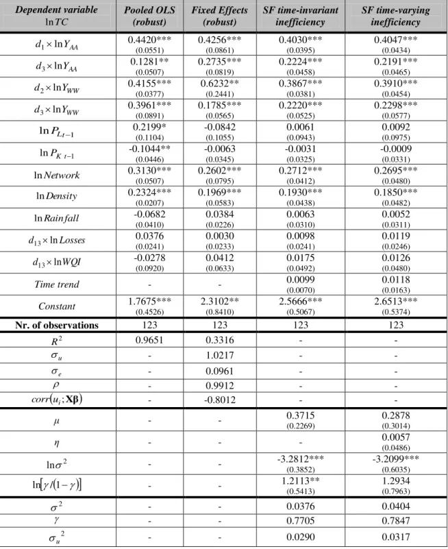
As mentioned before, depending on the estimation approach, the cost model may present slightly different specifications. In the next table, we present the estimation results for the
“preferred” specification for each econometric model:
Table 3 –Estimation results for the “preferred” specification for each econometric model
Dependent variable
TC
ln Pooled OLS (robust)
Fixed Effects (robust) SF time-invariant inefficiency SF time-varying inefficiency AA Y
d1ln 0.4420***
(0.0551) 0.4256*** (0.0861) 0.4030*** (0.0395) 0.4047*** (0.0434)
AA
Y
d3ln 0.1281**
(0.0507) 0.2735*** (0.0819) 0.2224*** (0.0458) 0.2191*** (0.0465)
WW
Y
d2ln 0.4155***
(0.0377) 0.6232** (0.2441) 0.3867*** (0.0381) 0.3910*** (0.0454)
WW
Y
d3ln 0.3961***
(0.0891) 0.1785*** (0.0565) 0.2220*** (0.0525) 0.2298*** (0.0577)
1
lnPLt 0.2199* (0.1104) -0.0842 (0.1055) 0.0061 (0.0943) 0.0092 (0.0975)
1
lnPKt -0.1044** (0.0446) -0.0063 (0.0345) -0.0031 (0.0325) -0.0009 (0.0331)
Network
ln 0.3130*** (0.0507) 0.2602*** (0.0795) 0.2712*** (0.0412) 0.2695*** (0.0480)
Density
ln 0.2324***
(0.0207) 0.1969*** (0.0583) 0.1930*** (0.0438) 0.1850*** (0.0482)
fall Rain
ln -0.0682
(0.0410) 0.0384 (0.0226) 0.0063 (0.0310) 0.0052 (0.0311) Losses
d13ln 0.0376
(0.0241) 0.0030 (0.0233) 0.0098 (0.0241) 0.0119 (0.0246) WQI
d13ln -0.0278
(0.0920) 0.0412 (0.0633) 0.0175 (0.0492) 0.0126 (0.0480)
Time trend - - 0.0099 (0.0070) 0.0118 (0.0163)
Constant 1.7675*** (0.4526) 2.3102** (0.8410) 2.5666*** (0.5067) 2.6513*** (0.5374)
Nr. of observations 123 123 123 123
2
R 0.9651 0.3316 - -
u
- 1.0217 - -
e
- 0.0961 - -
- 0.9912 - -
ui;Xβ
corr - -0.8012 - -
μ - - 0.3715 (0.2269) 0.2878 (0.3014)
η - - - 0.0057 (0.0486)
2
ln - - -3.2812*** (0.3852) -3.2099*** (0.6035)
/1
ln - - 1.2113** (0.5413) 1.2934 (0.7963) 2
- - 0.0376 0.0404
- - 0.7705 0.7847
2
u
-19-Firstly, Pooled OLS was used to evaluate the impact of average elevation and water sources in
total costs. Regardless of the operator’s type (AA only, WW only or AA and WW), a hilly topography is expected to increase total costs via higher pumping costs. In what concerns the dummies for water sources, we would expect a negative sign for groundwater abstraction only and a positive sign if only surface water is used. Although not reported in Table 3, these variables were shown to be statistically insignificant when included in the regression. Regarding hilly topography, the effect is perhaps negligible: while in theory it could have an impact, in practice it is not an important determinant of costs. As far as we know, in the only paper where this factor is accounted for (Zschille and Walter, 2011), the authors found a positive and statistically significant impact. On the other hand, the impact of water sources could have been studied using an alternative variable if better data were available. For example, it would be preferable to have the shares of each type of water input, since the majority of operators uses water from both sources. When we introduce year dummies, although the estimated coefficients are positive, they are not statistically significant as well. Moreover, rainfall, water losses and water quality also do not explain well total costs.
In the Pooled OLS estimation, the coefficients on outputs and price of labor are significant and consistent with economic theory: higher levels of output and a higher price of labor will raise total costs. Despite of being statistically significant, the coefficient on the price of capital is unexpected. In general, Pooled OLS is not the most efficient way to explore jointly the within (time dimension) and between (individual dimension) variability of data. If the appropriate model is FE, it will yield biased and inconsistent estimators.
2
v
- - 0.0086 0.0087
The output reports the estimates for the coefficients and several parameters. Standard errors are clustered at the firm level and appear between brackets.
-20-Secondly, we estimated our cost model by FE. For every specification, the Hausman Test was performed and allowed us to conclude that FE is always preferred to RE. As well as in the Pooled OLS estimation, panel-robust standard errors were used in order to adjust for heteroskedasticity. Although the clustered robust standard errors are slightly larger, the estimated coefficients remain practically unchanged. Regarding output quantities, we reach the same conclusions as in Pooled OLS, but input prices are now statistically insignificant, raising the possibility that price differences are not important in explaining total costs. Under FE estimation, we can conclude that average annual rainfall, water quality, water losses and year dummies apparently do not have a role in explaining total costs. Additional information can be extracted from the FE regression output. The standard deviation of residuals within operators
u 1.0217
is approximately 11 times higher than the standard deviation of overall residuals
e 0.0961
. The fraction of variance due to residuals within operators,
2 2
99%2
u u e
, tells us that practically all variance is due to considerable differences from one operator to another in terms of data variation. Finally, the empirical correlation between the errors within operators and the set of regressors, corr
ui;Xβ
, is about -0.8012 (under RE this correlation is 0 by assumption). Nevertheless, least squares-based regression techniques, such as Pooled OLS, FE or RE, estimate cost functions assuming that deviations from cost-minimizing behavior are attributed exclusively to random statistical noise. Those approaches do not consider that each firm potentially expends more than it should due to an inherent degree of inefficiency. Therefore, it is useful to estimate our cost model under a last approach – Stochastic Frontier Analysis (SFA).
-21-(“Battese-Coelli model”). Considering the two specifications, there are no significant differences between the estimated coefficients. As already expected, a higher level of output will result in higher costs. As in FE, input prices are not statistically significant. We note that under every approach (Pooled OLS, FE and SFA), the coefficients on network length and density (proxy for population density) always have a positive and statistically significant impact on total costs. Regarding network length, it just confirms our prediction: more kilometers of network mean higher costs. On the other hand, the positive sign on density points out that it is not more costly to serve more dispersed consumers, thus contradicting our initial belief. Under SFA, rainfall, water losses and water quality are not statistically significant.
The SFA outputs also provide us some parameters of interest. The estimate on 2, the total variance disturbance
2 2 2
v
u
, can be used as a measure of the goodness of fit – the best model specification is the one with lower overall disturbance. The very high estimates of
, which is defined as 2
2 2
v u
u
-22-the bulk level in -22-the Portuguese water sector. Since -22-the coefficients are not statistically significant, we can conclude for the absence of technological change during the period under analysis (2004-2011). Although the time-invariant hypothesis is somewhat restrictive because, hopefully, managers learn from past experience, we found evidence that operators kept their levels of inefficiency constant over time. As explained before, this is a reasonable hypothesis in the context of non-competitive environments, such as the water sector.
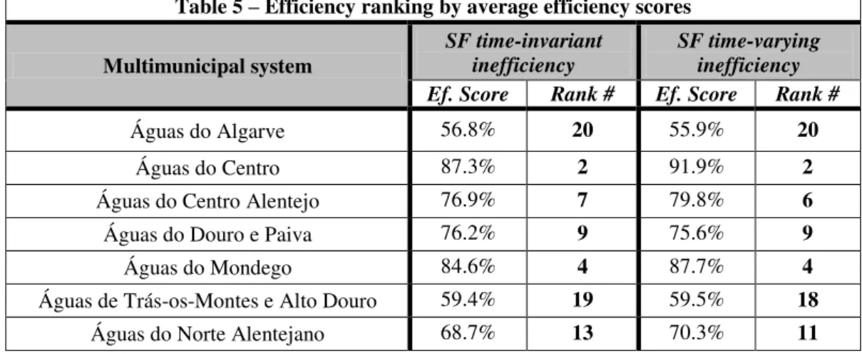
Under SFA, we can obtain operators’ efficiency scores, which can be used for benchmarking
purposes. Using the expression derived in Section 4, the average efficiency scores per type of operator are presented in the next table:
Table 4 – Average efficiency scores per type of operator
Selected model AA only WW only AA and WW Overall
SF time-invariant inefficiency 80.3% 73.9% 71.1% 73.1% SF time-varying inefficiency 80.1% 76.9% 71.3% 74.0%
The efficiency scores were obtained from the SF regressions presented in Table 3. Due to the different specifications for the inefficiency term, the individual efficiency scores will be constant over time under the time-invariant model. This comes from the assumption that operator i is as inefficient in t 1as in t 2;3;;T.On the other hand, in the time-varying model, each operator will have an efficiency score for every year of activity. In the next table, we present the ranking of multimunicipal systems by average efficiency scores:
Table 5 – Efficiency ranking by average efficiency scores
Multimunicipal system
SF time-invariant inefficiency
SF time-varying inefficiency Ef. Score Rank # Ef. Score Rank #
Águas do Algarve 56.8% 20 55.9% 20
Águas do Centro 87.3% 2 91.9% 2
Águas do Centro Alentejo 76.9% 7 79.8% 6
Águas do Douro e Paiva 76.2% 9 75.6% 9
Águas do Mondego 84.6% 4 87.7% 4
Águas de Trás-os-Montes e Alto Douro 59.4% 19 59.5% 18
-23-Águas do Oeste 67.1% 14 67.9% 14
Águas do Zêzere e Côa 72.5% 11 74.7% 10
SANEST 63.1% 17 64.0% 16
SIMARSUL 76.4% 8 78.8% 8
SIMLIS 85.7% 3 91.7% 3
SIMRIA 79.9% 5 84.6% 5
SIMTEJO 64.3% 16 65.4% 15
Águas do Ave 59.7% 18 57.1% 19
Águas do Cávado 94.8% 1 95.8% 1
Águas do Minho e Lima 78.2% 6 79.2% 7
Águas do Noroeste 75.2% 10 63.6% 17
EPAL –“bulk” 69.8% 12 69.0% 12
Águas de Santo André –“bulk” 66.2% 15 67.9% 13
-24-6- Conclusion.
This paper aimed at studying the cost efficiency of multimunicipal systems operating at the bulk level in the Portuguese water sector. Under every approach (Pooled OLS, FE and SFA), higher output quantities are expected to raise total costs. It can also be concluded that input prices –
usually included to capture regional price differences – do not seem to have a significant influence in total costs. This conclusion is in line with the findings of Correia (2008) and corroborates the hypothesis of Martins, Fortunato and Coelho (2005), when they state that regional differences in prices are small in a small country like Portugal. Additionally, average rainfall, water losses and water quality apparently do not play a role in explaining operators’
total costs. Contrarily to our initial belief, the sign of the coefficient on density suggests that it is not more costly to serve more dispersed consumers. Regarding water sources and average elevation, they have shown to be irrelevant when Pooled OLS was performed. Since the time-decay parameter is close to 0 and statistically insignificant, the time-invariant inefficiency model seems to be the most appropriate. We also found that inefficiency of operators remained constant over time, which is not an encouraging conclusion. The main source of the distance to the cost frontier is a high degree of inefficiency and not exogenous random shocks. However, average efficiency scores are not very far from those presented in other studies for developed countries. Since single product operators present higher average efficiency scores, there is also some evidence for gains from specialization.
-25-References
Aigner, Dennis, C. A. Knox Lovell and Peter Schmidt. 1977. “Formulation and Estimation
of Stochastic Frontier Production Function Models.” Journal of Econometrics, 6(1): 21-37. Bain, Joe. 1956. Barriers to New Competition. Cambridge, MA: Harvard University Press. Battese, G. E., and T. J. Coelli. 1992. “Frontier production functions, technical efficiency and panel data: With application to paddy farmers in India.” Journal of Productivity Analysis, 3(1): 153-169.
Bottasso, Anna and Maurizio Conti. 2003. “Cost Inefficiency in the English and Welsh
Water Industry: An Heteroskedastic Stochastic Cost Frontier Approach.” Economics discussion
papers 573, University of Essex, Department of Economics.
Cameron, A. Colin and Pravin K. Trivedi. 2009. Microeconometrics – Methods and
Applications, 8th edition, New York: Cambridge University Press, pp. 697-778.
Coelli, T. J. and Shannon Walding. 2005. “Performance Measurement in the Australian
Water Supply Industry.” Centre for Efficiency and Productivity Analysis (CEPA), Working Paper Series No. 01/2005, School of Economics, University of Queensland, St. Lucia Australia. Coelli, T. J., D.S. Prasada Rao, Christopher J. O'Donnell and G. E. Battese. 2005. An Introduction to Efficiency and Productivity Analysis, 2nd Edition, Springer, New York, pp. 241-288.
Correia, Tânia. 2008. “Eficiência dos Serviços de Água e de Águas Residuais em Portugal – Aplicação da Análise de Fronteira Estocástica.” Dissertação para a obtenção do Grau de Mestre
em Engenharia Civil, Instituto Superior Técnico, Universidade Técnica de Lisboa, Portugal. Filippini, M., Nevenka Hrovatin and Jelena Zoric. 2007. “Cost Efficiency of Slovenian Water Distribution Utilities: An Application of Stochastic Frontier Methods.” 19th SIEP
Conference – Human Capital Economics, September 13-14, Pavia, Italy.
Fraquelli, Giovanni and Valentina Moiso. 2005. “Cost efficiency and economies of scale in the Italian Water Industry.” 17th SIEP Conference – Public Sector Financing, September 15-16,
Pavia, Italy.
Krause, Mathias. 2009. The Political Economy of Water and Sanitation. New York: Routledge.
Kumbhakar, S. C., and C. A. K. Lovell. 2000. Stochastic Frontier Analysis. Cambridge: Cambridge University Press.
Lin, Chen. 2005. “Service Quality and Prospects for Benchmarking: Evidence from the Peru Water Sector.” Utilities Policy, 13(3): 230-239.
Martins, Rita, Adelino Fortunato and Fernando Coelho. 2006. “Cost Structure of the
Portuguese Water Industry: A Cubic Cost Function Approach.” Group of Monetary and Fiscal
Studies (GEMF), Working Paper No. 9, Faculty of Economics, University of Coimbra, Portugal.
Varian, Hal R. 2010. Intermediate Microeconomics: A Modern Approach, 8th edition, New York: W. W. Norton & Company, pp. 332-394.
Walter, Mathias, Astrid Cullmann, Christian von Hirschhausen, Robert Wand and Michael Zschille. 2009. “Quo vadis efficiency analysis of water distribution? A comparative literature review.” Utilities Policy, 17(3-4): 225-232.
Zschille, Michael and Matthias Walter. 2011. “The Performance of German Water Utilities:
A (Semi)-Parametric Analysis”. Discussion Papers of DIW Berlin 1118, German Institute for