Principal Component Analysis applied to
digital image compression
Utilização da Análise de Componentes Principais na compressão de imagens digitais
Rafael do Espírito Santo*
Study carried out at Instituto do Cérebro – InCe, Hospital Israelita Albert Einstein – HIAE, São Paulo (SP), Brazil.
* Instituto do Cérebro - InCe, Hospital Israelita Albert Einstein – HIAE, São Paulo (SP), Brazil.
Corresponding author: Rafael do Espírito Santo – Avenida Morumbi, 627/701 – Morumbi – Zip code: 05651-901 – São Paulo (SP), Brazil – Phone: (55 11) 2151-1366 – Fax: (55 11) 2151-0273 – E-mail: rafaeles@einstein.br
Received on: Sep 5, 2011 – Accepted on: Jun 13, 2012 Conflict of interest: none.
ABSTRACT
Objective: To describe the use of a statistical tool (Principal Component Analysis – PCA) for the recognition of patterns and compression, applying these concepts to digital images used in Medicine. Methods: The description of Principal Component Analysis is made by means of the explanation of eigenvalues and eigenvectors of a matrix. This concept is presented on a digital image collected in the clinical routine of a hospital, based on the functional aspects of a matrix. The analysis of potential for recovery of the original image was made in terms of the rate of compression obtained. Results: The compressed medical images maintain the principal characteristics until approximately one-fourth of their original size, highlighting the use of Principal Component Analysis as a tool for image compression. Secondarily, the parameter obtained may reflect the complexity and potentially, the texture of the original image. Conclusion: The quantity of principal components used in the compression influences the recovery of the original image from the final (compacted) image.
Keywords: Principal component analysis; Eigenvalues; Eigenvectors; Image compressing; Patters; Dimensionality reduction
RESUMO
Objetivo: Descrever a utilização de uma ferramenta estatística (Análise de Componentes Principais ou Principal Component Analysis – PCA) para reconhecimento de padrões e compressão, aplicando esses conceitos em imagens digitais utilizadas na medicina. Métodos: A descrição da Análise de Componentes Principais é realizada por meio da explanação de autovalores e autovetores de uma matriz. Esse conceito é apresentado em uma imagem digital coletada na rotina clínica de um hospital, a partir dos aspectos funcionais de uma matriz. Foi feita a análise de potencial para recuperação da imagem original em termos de taxa de compressão obtida. Resultados: As imagens médicas comprimidas mantêm as características principais até aproximadamente um quarto de seu volume original, destacando
o emprego da Análise de Componentes Principais como ferramenta de compressão da imagem. Secundariamente, o parâmetro obtido pode refletir a complexidade e, potencialmente, a textura da imagem original. Conclusão: A quantidade de componentes principais utilizada na compressão influencia a recuperação da imagem original a partir da imagem final (compactada).
Descritores: Análise de componentes principais; Autovalores; Autovetores; Compressão de imagens; Padrões; Redução de dimensão
INTRODUCTION
Principal Components Analysis (PCA)(1) is a
mathematical formulation used in the reduction of
data dimensions(2). Thus, the PCA technique allows the
identification of standards in data and their expression in such a way that their similarities and differences are emphasized. Once patterns are found, they can be compressed, i.e., their dimensions can be reduced without much loss of information. In summary, the PCA formulation may be used as a digital image compression algorithm with a low level of loss.
In the PCA approach, the information contained in a set of data is stored in a computational structure with reduced dimensions based on the integral projection of the data set onto a subspace generated
by a system of orthogonal axes(3). The optimal system
of axes may be obtained using the Singular Values
Decomposition (SVD) method(4). The reduced
dimension computational structure is selected so that relevant data characteristics are identified with little
loss of information(3). Such a reduction is advantageous
representation, calculation reduction necessary in subsequent processing, etc.
Use of the PCA technique in data dimension reduction is justified by the easy representation of multidimensional data, using the information contained in the data covariance matrix, principles of linear
algebra(3) and basic statistics. The studies carried out
by Mashal et al.(5) adopted the PCA formulation in
the selections of images from a multimedia database.
According to Smith(6), PCA is an authentic image
compression algorithm with minimal loss of information. The relevance of this work is in the performance evaluation of the PCA formulation in compressing digital images from the measurement of the degree of compression and the degree of information loss that the PCA introduces into the compressed images in discarding some principal components.
OBJECTIVE
This article has the purpose of describing the PCA of a population of data and the possibility of applying it to the compression of digital images. The application of the technique in pattern recognition is also emphasized.
METHODS
Digital images
Admitting digital processing, a continuous (analogical) datum is converted into a matrix of simple elements (pixels) that assume discrete values (gray levels), that is:
(expression 1)
In which the values of x and y (x, y) are the
coordinates of the pixels in the image, and f(x,y) is the
corresponding level of gray(7).
COVARIANCE Of AN IMAGE
The covariance matrix of an image is given by:
covImg = f(x,y)*f(x,y)T3 (expression 2)
PCA
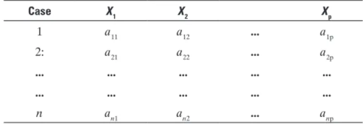
A PCA may be characterized from the data of p variables
for n individuals, as is indicated on table 1.
By definition(1), the first principal component is the
linear combination of variables X1X2;...;Xp, that is,
Z1 = a11X1 + a12X2 +... + a1pXp (expression 3)
The second principal component
Z2 = a21X1 + a22X2 +... + a2pXp (expression 4)
Table 1. Format of data for a Principal Component Analysis from n observations of variables X1 and Xp
Case X1 X2 Xp
1 a11 a12 ... a1p
2: a21 a22 ... a2p
... ... ... ... ...
... ... ... ... ...
n an1 an2 ... anp
The third principal component,
Z3 = a31X1 + a32X2 +... + a3pXp (expression 5)
and so forth. If there are p variables, then there are
at most p principal components, always calculated
according to expressions similar to expressions (3) or (4) or (5).
The results of a PCA, that is, the principal
components Zp are obtained from an analysis that
consists in finding the eigenvalues(3-6) of a sample
covariance matrix(8). The covariance matrix is
symmetrical and has the form:
(expression 6),
in which the elements cjj, positioned along the primary
diagonal, are the variances of Xi (var(Xi))and the cij’s of the secondary diagonal represent the covariance between the variables Xi Xj (cov (Xi, Xj)).
The eigenvalues of matrix C are the variances of
the principal components. There are p eigenvalues.
They are always numbers greater than or equal to zero,
represented by the symbol λ. Negative λ’s are not allowed
in a covariance matrix(6). Assuming that the eigenvalues
are ordered as λ1>λ2>...λp> 0, then λ1corresponds to
the first principal component (expression 1), and λi to
the i-th principal component, or:
As was mentioned, var(Zi) = λi and the constants
ai1, ai2,..., aip are the elements of the corresponding
eigenvector, graduated so that(6)
(expression 8)
The fact that cii is the variance of Xi and that λi is the
variance of Zi implies that the sum of variances of the
principal components is equal to the sum of variances
of the original variances(6). Thus, in a way, the principal
components contain all the variation of the original data(5,6).
The steps normally followed in a PCA of a digital image can now be established:
Step 1: In the computational model of a digital image, in expression 1, the variables X1, X2,...,Xpare the columns of the image. The PCA is begun by coding (correcting) the image to that its columns have zero means and unitary variances. This is common, in order to avoid one or the other of the columns having undue influence on
the principal components(6):
image corrected by the mean = image – mean of the image
(expression 9)
Step 2: The covariance matrix C is calculated using expression 6, implemented computationally, that is:
covImage = image corrected by the mean ×
(image corrected by the mean)T (expression 10)
Step 3: The eigenvalues λ1,λ2,...,λp and the corresponding eigenvectors a1, a2,..., ap. are calculated.
Step 4: The value of a vector of characteristics is obtained, a matrix with vectors containing the list of eigenvectors
(matrix columns) of the covariance matrix(6).
vc = (av1, av2, av3,..., avn) (expression 11)
Step 5: The final data are obtained, that is, a matrix with all the eigenvectors (components) of the covariance matrix.
finaldata = vcT× (Image - mean)T (expression 12)
Step 6: The original image is obtained from the final data without compression using the expression
Image T = (vc)T× finaldata + meanT (expression 13)
Step 7: Any components that explain only a small portion of the variation in data for the effect of image
compression are discarded. The eliminations have the effect of reducing the quantity of eigenvectors of the characteristics vectors and can produce final data with a smaller dimension. The use of expression 13 in these conditions allow the recovery of the original image with compression.
Compression rate
According to Castro(9,10), low-loss compression
afforded by the present method may be expressed in
terms of the compression factor of (ρ) and of the mean
squared error (MSE) committed in the approximation
of A (original image) by à (image obtained from the
disposal of some of the components). The compression factor is defined by:
(expression 14)
And the MSE committed in the approximation of
A byà is:
MSE =
(expression 15)
RESULTS
This section shows examples of compression of digitalized images using the PCA formulation. Various situations are presented as examples.
Example 1: Recovering a TIFF image with 512x512 pixels with all the components (512) of image covariance matrix (without compression, i.e., steps 1 to 6).
Recovered image (512x512 pixels) from 512 principal components
Memory necessary (final data)=512x512=262144 units of memory Compression factor (ρ)=262144/262144=1
Compression rate (1-ρ)=1-1=0 Mean squared error (MSE)=0
Example 2: Recovery of a TIFF image with 512x512 pixels with 112 principal components of the covariance matrix of the image (with compression, that is, steps from 1 to 5 to 7).
Original image: TIff with 512x512 pixels*
Image recovered (512x512 pixels) from 112 principal components
Memory necessary (final data)=112x512=57344 units of memory Compression factor (ρ)=57344/262144=0.219
Compression rate (1-ρ)=1-0.219=0.781 Mean squared error (MSE)=0213
Example 3: Recovery of an image with 32 principal components of the image covariance matrix (with compression).
Original image: TIff with 512x512 pixels*
Recovered image (512x512 pixels) from 32 principal components
Memory necessary (final data)=32x512=16384 units of memory Compression factor (ρ)=16384/262144=0.0625
Compression rate (1-ρ)=1-0.0625=0.9375 Mean squared error (MSE)=0.8825
Example 4: Recovery of an image with 12 principal components of the covariance matrix of the image (with compression).
Recovered image (512x512 pixels) from 12 principal components
Memory necessary (final data)=12x512=6144 units of memory Compression factor (ρ)=6144/262144=0.0234
Compression rate (1-ρ)=1-0.0234=0.9766 Mean squared error (MSE)=0.9505
* Structural image of the brain acquired at the Magnetic Resonance Department of Hospital Israelita Albert Einstein. The im-age was acquired using a T1-weighted Spoiled Gradient Recalled Asymmetric Steady State (SPGR) sequence, in a magnetic resonance clinical examination apparatus from GE Sigma LX 1.5T (Milwaukee, USA). One hundred and twenty eight 1-mm isotropic slices of the cerebral cortex were acquired.
DISCUSSION
Examples 1 to 4 show the effects of the reduction in number of principal components (elevation of the image compression rate) in the increased loss of information. This application may bring great savings in storage of medical images. However, the level of information preserved depends on the parameters (compression rate), and should be modulated by the user’s interest. The higher the compression rate (the fewer principal components are used in the characteristics vector) the more degraded the quality of the image recovered (examples 3 and 4).
In certain applications, such as brain function images, the central principle is the variation of the resonance signal over time. In these conditions, the spatial information may be maintained in a reference file, making it possible to compress subsequent images with no loss. On the other hand, it is still necessary to evaluate the pertinence of the application of high compression rates when an assessment of structures of
reduced dimensions relative to the size of the voxelsis
needed.
Furthermore, the observation of the results from the application of the PCA technique in medical images may be considered a complexity measure. In other words, images with dense texture patterns tend to produce different results with the use of the
technique described. Nevertheless, this hypothesis was not tested in this project; it only points to the line of investigation, in which the results may certify and quantify this possibility.
New secondary applications (based on the results here described) may encompass various conditions in the medical routine. These applications benefit from the procedures described herein. In this way, the comprehension of the principles here presented is important for the better use of medical applications based on these foundations.
CONCLUSION
The quantity of principal components used in compression influences the recovery of the original image from the compacted image. This tool allows significant savings of storage space, which can be critical in clinical applications and in processing large volumes of data. As a secondary property, these components also have the potential of reflecting the complexity of the image, enabling their correlation with the texture of the image.
REfERENCES
1. Haykin S. Neural networks: a comprehensive foundation. New York: Prentice Hall; 1999.
2. Jolliffe IT. Principal component analysis. New York: Springer-Verlag; 1986. 3. Ye J, Janardan R, Li Q. GPCA: an efficient dimension reduction scheme for image
compression and retrieval [Internet]. In: Conference on Knowledge Discovery in Data Proceedings of the tenth ACM SIGKDD international conference on Knowledge discovery and data mining. Seattle (WA); 2004. [cited 2012 Apr 12]. Available in: http://www.public.asu.edu/~jye02/Publications/Papers/ gpca-kdd04.pdf
4. Golub GH, Van Loan CF. Matrix computations. 3rd ed. Baltimore (MD): The Johns Hopkins University Press; 1996.
5. Mashal N, Faust M. Hendler T. The role of the right hemisphere in processing nonsalient metaphorical meanings: application of principal components analysis to fMRI data. Neuropsychologia. 2005;43(14):2084-100.
6. Smith LI. A tutorial on principal components analysis [Internet]. 2002 [cited 2011 May 22]. Available in: http://www.sccg.sk/~haladova/principal_ components.pdf
7. Gonzalez RC, Woods RE. Digital imaging processing. Massachusetts: Addison-Wesley; 1992.
8. Boldrini JL, Costa CR, Figueirado VL, Wetzler HG. Álgebra linear. 3a ed. São Paulo: Harbra; 1984.
9. Castro MC. Algoritmo herbiano generalizado para extração dos componentes principais de um conjunto de dados no domínio complexo [dissertação]. Porto Alegre: Pontifícia Universidade Católica do Rio Grande do Sul; 1996. 10. Castro MC, Castro FC. Codificação de sinais. 2008. Disponível em: http://