José Miguel Pinheiro da Silva Pinto
Licenciado em Ciências da Engenharia Electrotécnica e de Computadores
Solving the Travelling Salesman Problem based
on Coupled Ring-Oscillators
Dissertação para obtenção do Grau de Mestre em Engenharia Electrotécnica e de Computadores
Orientador: Prof. Doutor João Carlos da Palma Goes,
Professor Catedrático, Universidade Nova de Lisboa
Júri
Presidente: Doutor Rodolfo Alexandre Duarte Oliveira Arguente: Doutor Raúl Eduardo Capelo Tello Rato
Solving the Travelling Salesman Problem based on Coupled Ring-Oscillators Copyright © José Miguel Pinheiro da Silva Pinto, Faculdade de Ciências e Tecnologia, Universidade NOVA de Lisboa.
A Faculdade de Ciências e Tecnologia e a Universidade NOVA de Lisboa têm o direito, perpétuo e sem limites geográficos, de arquivar e publicar esta dissertação através de exemplares impressos reproduzidos em papel ou de forma digital, ou por qualquer outro meio conhecido ou que venha a ser inventado, e de a divulgar através de repositórios científicos e de admitir a sua cópia e distribuição com objetivos educacionais ou de inves-tigação, não comerciais, desde que seja dado crédito ao autor e editor.
Este documento foi gerado utilizando o processador (pdf)LATEX, com base no template “novathesis” [1] desenvolvido no Dep. Informática da FCT-NOVA [2]. [1]https://github.com/joaomlourenco/novathesis [2]http://www.di.fct.unl.pt
Ac k n o w l e d g e m e n t s
Firstly I would like to acknowledge and deeply thank my adviser Professor João Goes for allowing me to try and punch above my weight with this project and being present for any doubts, questions and mental rambling that showed up during the past year and a half. I would also like to stretch this first thanks to Professor Luís Oliveira that has been an inspiration and guide during the years I have been enrolled in this masters degree, allowing me to take a deeper instruction in the world of electronics, suggesting me to this amazing project and always having an open door for when the fighting got tough. Finalising the acknowledgements to the academic world I have to mention all of the professors that have crossed my path in FCT/UNL and at TU Wien.
Secondly I would like to thank my friends and colleagues that since the first classes until the day this thesis was delivered took some of their time to make me laugh and question the world.
A very special thank you goes to the members of NAve and the Suicide Squad that have allowed for a physical and mental escape from an academic world that would definitely have broken my mind if I had not found climbing, slacklining, snowboarding and so many other ways to incorporate the outdoors in my academic life.
A truly heartfelt thank you goes to my Scouting group and the friend that came from that big part of my life that constantly worry about me and challenge me to be a better version of myself.
Last, but never least, the Family. First the family you chose: Ayala, Duda, Filipe, Inês, Lopes, Ricardo, Tiago and so many others that would take their time to discuss expensive beer, play boardgames, hike for days with swollen feet or simply dive deeper into the recesses of the human mind.
To the family you couldn’t choose but fit into perfectly: like my parents, Élia and José, that have done everything to allow me to study whatever I felt like and inspired me to achieve more and more through their exemplary dedication; my grandparents Alonso and José that have, each in their own world, showed me what dedication to your work and family means and unfortunately will never see me work as hard as they have; my grandmas Ana and Clarisse that still today teach me more about life; and finally my sister Joana that could probably fit into any of this groups as she’s an Inspirational Academic, FCT alumni, badass climber, scouts "mini-Leader"and my longest-lasting friend.
To all of you, my deepestObrigado.
A b s t r a c t
When thinking of hard mathematical problems the notion of NP-hard usually comes into play. One of the most famous NP-hard problems is the Travelling Salesman Problem (TSP), which tries to solve the following: Given a list of cities and distances in-between them, what is the shortest possible route that visits every city and returns to the original city?
This common optimisation problem has some heuristics and approximation algo-rithms that can help solve it but most solutions still have an exponential increment of time and complexity with every city that is added.
By encoding a TSP into a circuit designed with coupled ring oscillators and by analysing the frequency spectra throughout the time we hoped to be able to determine the shortest path that would connect all of the cities.
Our test were unable to solve a complete TSP but we were in fact able to prove some landmark points of our implementation that could help to solve it. Namely we showed that in our cases higher frequencies spread quicker, multiple frequencies can be spread through a single ring oscillator and these frequencies actually spread throughout the circuit.
Some suggestions are made of possible future work and we also take note on some of the limitations of this project.
Keywords: Ring Oscillators, Travelling Salesman Problem, Coupling, Oscillatory com-puting, Optimisation
R e s u m o
A noção de problemas NP-complexo surge rapidamente quando se pensam em pro-blemas matemáticos de difícil resolução. Um dos mais famosos destes propro-blemas é o Problema do Caixeiro Viajante, que tenta resolver o seguinte: Dada uma lista de cidades e a distância entre as mesmas, qual é a rota mais pequena que visite todas as cidades e volte ao ponto de partida?
Existem alguns métodos heurísticos e algoritmos de aproximação que permitem obter uma resposta aproximada do problema. No entanto, estes métodos mantêem a complexi-dade exponencial associada ao adicionar de cada nova cicomplexi-dade.
Tentámos, portanto, nesta tese, codificar um simples caso do Problema do Caixeiro Viajante num circuito desenhado com osciladores em anel acoplados no qual analisámos os espectros de frequência ao longo do tempo com a ideia de conseguir determinar o caminho mais curto para ligar todas as cidades.
Nos nossos testes não conseguimos resolver um problema completo, mas conseguimos provar alguns pontos da nossa ideia que achamos poderem ajudar numa futura imple-mentação. Nomeadamente comprovámos que frequências mais altas se espalham mais rapidamente, múltiplas frequências podem-se espalhar por um único oscilador em anel e que estas frequências se espalham de facto ao longo do circuito.
São também realçadas algumas das limitações do projecto bem como trabalho futuro que pode ser feito.
Palavras-chave: Osciladores em Anel, Problema do Caixeiro Viajante, Acoplamento, Computação com Osciladores, Optimização
C o n t e n t s
List of Figures xv
List of Tables xvii
Acronyms xix
1 Introduction 1
1.1 Motivation . . . 1
1.2 Organization . . . 3
1.3 Contributions . . . 3
2 State of the Art: Models and Applications 5 2.1 Simulated Annealing . . . 5
2.2 Ising Computing. . . 7
2.3 CMOS Annealing . . . 7
2.4 Quantum Annealing . . . 8
2.5 Oscillator Based Computing . . . 8
2.5.1 Spin-Torque Oscillators. . . 9
2.5.2 Vanadium Dioxide Oscillators . . . 10
3 Elements and Proposed Idea 11 3.1 Elements Used . . . 11
3.1.1 Ring Oscillators and their Working Principle . . . 11
3.1.2 Coupling of RO . . . 13
3.1.3 Filters. . . 15
3.2 Proposed Idea . . . 15
3.2.1 Working Principle. . . 16
4 Circuit Implementation and Simulation Results 19 4.1 Circuit Implementation . . . 19 4.1.1 Cities . . . 19 4.1.2 Paths . . . 20 4.1.3 Coupling . . . 21 4.2 Methods of Analysis . . . 22 xiii
C O N T E N T S
4.2.1 Time Swept FFT . . . 23
4.3 Simulation Results. . . 24
4.3.1 Faster Frequencies Arrive Faster. . . 24
4.3.2 The circuit redirects multiple frequencies . . . 26
4.3.3 The Frequencies are passed from city to city . . . 28
5 Conclusions and Future Work 31 5.1 Conclusions . . . 31
5.2 Future Work . . . 32
Bibliography 33
I Annex 1 - MATLAB code 37
II Annex 2 - Cadence Virtuoso Circuits 39
L i s t o f F i g u r e s
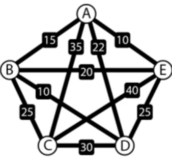
1.1 Graph of the 5 city TSP initially used in this thesis. . . 2
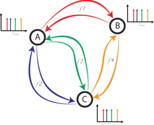
1.2 Graph of the 3 city TSP with each arrow indicating an unidirectional path, at this point no distances were chosen. Each colour represents a different frequency. . . 2
2.1 An example containing 10 particles in a regular lattice. . . 6
2.2 The selected particle can move to any part of the smaller square. . . 6
3.1 Assembly of a ring oscillator, where n can be any natural number or zero. . . 11
3.2 Design of an Inverter. . . 12
3.3 Frequency of oscillation based on the number of inverters at a fixed size. . . 13
3.4 Phase noise analysis of a RO. . . 14
3.5 Design of a coupler. . . 14
3.6 Layout of UMC130nm inductors for our edge cases, to the left a 371pH induc-tor and to the right a 5.842nH inducinduc-tor. . . . 15
3.7 After some time we should be able to see all of the frequencies in all of the cities. . . 17
4.1 RO representing a city. . . 20
4.2 Schematic of an inverter with voltage supply of 1.2V and −1.2V . . . 21
4.3 The coupling of a City to a Path with 3 different Bandpass Filters. . . 22
4.4 Schematic of how the Time Swept FFT works. . . 23
4.5 For this test we have two different paths connected to one city. . . 24
4.6 Circuit with 2 RO, representing two paths, coupled to the same city. . . 25
4.7 Representation of the test assembled to test this scenario. . . 26
4.8 Circuit with 2 RO, representing two paths, connected to the same city and then a third path connecting to another city. . . 27
4.9 Superposition of an FFT before and after turning on the first two paths. . . . 27
4.10 Representation of the test assembled to test this scenario. . . 28
4.11 FFT on City C after the circuit stabilised. . . 29
II.1 Circuit of a single inverter with multiplier at 5. . . 39
II.2 Circuit of a single inverter. . . 40
L i s t o f F i g u r e s
II.3 Circuit used to test which frequencies arrive before. We can see two big ring oscillators with an enabler that represent the cities and a smaller ring oscillator to represent one city. Two single inverters serve as buffer between the big RO and the smaller one. . . 41
II.4 Circuit used to test if we could connect two frequencies to a RO and have it spread. We can see attached to the same circuit as before one more large RO and a smaller one representing one more path and a city to connect to, respectively. . . 42
II.5 Circuit used to test if the frequencies ejected on the first city would spread. In this circuit we see 6 Ring Oscillators connected in series. It is important to notice the addition of the filters that was required in order to have proper results in the end. . . 43
L i s t o f Ta b l e s
4.1 Sizes used in the implementation of the cities’ inverters. . . 20
4.2 Sizes used in the implementation of the paths’ inverters. . . 20
4.3 Average values measured on the FFT for each signal. . . 25
4.4 Analysis of our TimeSwept FFT with 20 ns windows starting from 13.4ns to 14.4ns. . . 26
4.5 Analysis of our TimeSwept FFT with 20 ns windows starting from 19ns to 20ns. 26
4.6 Frequency of the different Paths used on test number 2. . . 27
4.7 Frequency of the different Paths used on test number 3. . . 28
Ac r o n y m s
CAD Computer-Aided Design.
FFT Fast Fourier Transform.
MOS Metal-Oxide-Semiconductor.
NMOS Negative-channel Metal-Oxide-Semiconductor.
PMOS Positive-channel Metal-Oxide-Semiconductor.
RO Ring Oscillator.
STO Spin-Torque Oscillators.
TSP Travelling Salesman Problem.
VO2 Vanadium Dioxide.
C
h
a
p
t
e
r
1
I n t r o d u c t i o n
1.1
Motivation
The Traveling Salesman Problem (TSP) is a problem of combinatorial mathematics with non-deterministic polynomial-type hardness (NP-hard) which can be easily enumerated as:
Given a collection of cities and the cost of travel between them, the Travelling Salesman Problem, is to find the shortest way to visit every city
and come back to the origin without visiting any city twice.
Whilst exposing the problem is fairly simple the problem get factorially harder to solve, as for each added city the number of possible routes increases factorially. In the end, the number of possible solutions to be analyzed when you have N cities, and after selecting a starting point, is of (N − 1)!/2, the division by two comes from the fact that the direction does not matter (As going through cities A-C-B-D-A is the same as going A-D-B-C-A)).
There are numerous real-life uses for the TSP from optimising the drilling of printed circuit boards or the order through which objects are picked up on a warehouse, to the most commonly thought vehicle routing. [12]
Given the large number of possible solutions that even a small TSP generates, it is impossible to solve them in polynomial time. With some methods, like the Held-Karp Algorithm, we can come down from O(n!) to O(2nn2), leaving us with exponential time instead of factorial. This means that completely solving a TSP still takes an excruciating amount of time, when using traditional computation methods.
Even with other algorithms it is hard to get optimal solutions with a time smaller than exponential, so, the solutions used nowadays evolve around heuristics and dynamic
C H A P T E R 1 . I N T R O D U C T I O N
programming leading to non-optimal but accurate enough solutions for daily problems. Having seen several new computational methods showing up on the last decades (see Chapter2for a deeper explanation) that have been used to solve harder and harder mathematical problems a choice was made to examine a different approach to the TSP.
With the problem present in our minds and given how difficult it is to solve it using normal computational methods we set on creating a methodology to solve a TSP using coupled ring oscillators that would allow us to solve every possible solution at the same time leading to an implementation which could probably have better results than the current methodologies.
The original goal behind this thesis was set on solving the 5-city TSP seen in Figure
1.1.
Figure 1.1: Graph of the 5 city TSP initially used in this thesis.
This goal was dismissed while we corrected some of the initial ideas of the implemen-tation and a decision was made to instead focus on the building blocks of the idea and explore them based on a 3 cities TSP like the one present in Figure 1.2.
Figure 1.2: Graph of the 3 city TSP with each arrow indicating an unidirectional path, at this point no distances were chosen. Each colour represents a different frequency.
The proposed idea encodes the distances between cities into specific frequencies by adjusting the number of inverters on the ring oscillator, and associating it to the length of each path. At the same time every city is also characterised by a ring oscillator. To emulate the connection of paths we coupled the RO representing the path to both the cities it intertwines.
With all the connections in order we should be able to compute the TSP solution by analysing the order by which the frequencies express themselves in the cities.
1 . 2 . O R G A N I Z AT I O N
The results were not as exceptional initially anticipated as we were unable to fully solve a TSP. We have however made reasonable work to prove some of the key points of the implementation.
1.2
Organization
This thesis consists of five chapters, the first one being the Introduction present on this chapter where we take a closer look to the motivation behind this project, its goals and possible contributions.
The second one consists of a state-of-the-art analysis for other solutions used to solve combinatorial problems from metaheuristics technologies like Simulated Anneal-ing, present in Section2.1, to more advanced methods as Quantum Annealing present in Section2.4, and finalising with other examples of Oscillatory Based Computing.
The third chapter explores the Proposed Idea, how we expect our system to behave and the tools used to do so, taking a closer look into the working principles of Ring Oscillators, their coupling and some filters.
On the fourth chapter we dive deeper into the implementation of the idea and take on several tests to try and prove some key points in regards to solving a TSP using ring oscillators.
The fifth and final chapter concludes the project and points valid options on future work while discussing some of the handicaps of our project.
1.3
Contributions
The search for alternative methods to classical computation that can allow for a faster and more economical way to solve larger and harder problems has been a thrilling theme in academia for some years.
With this thesis we had hoped to bring a new method into play that would allow to solve this specific combinatorial problem with an easy and cheap CMOS implementation, that could be compared to the solutions of other methods like quantum annealers.
We were unable to present a solution to a TSP, as the implementation of bi-directional paths brought us some problems, but we have been able to lay some groundwork that can help future implementations to have a known working base that can perform some key points.
C
h
a
p
t
e
r
2
S ta t e o f t h e A rt : Mo d e l s a n d A p p l i c a t i o n s
Traditional computing as lead the way problems are solved in the past. However, with the growth of computational loads, problems are starting to get too complex to solve using conventional computing architectures and that is where new paradigms of computing come to shine.
To fully solve problems like the TSP requires a computer to calculate all of the possi-ble combinations and then proceed to see which one is the cheapest of all. As the number of cases that need to be computed increases expectationally the computation time also increases. This is where different methodologies come in handy, as they can either cal-culate all of the possibilities quickly, making it so that the only part of the problem is to find which one of the possible paths is the cheapest, or cut corners by achieving not the cheapest of solutions but one that is not too far from it.
There has been a lot of research into speeding up the computation of combinatorial problems using different technologies, in this chapter we will try to understand this technologies better.
2.1
Simulated Annealing
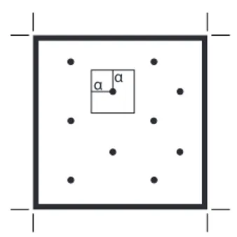
In his 1953 paper Metropolis proposes a method later known as the Metropolis Algorithm [17]. The idea behind the method is to simulate the interactions of individual molecules and trying to achieve a minimum energy state, so in this method N particles are placed in any configuration, an example can be seen in figure2.1.
From their original positions each particle moves, in succession according to (2.1).
X → X + αε1 (2.1)
Y → Y + αε2
C H A P T E R 2 . S TAT E O F T H E A R T: M O D E L S A N D A P P L I C AT I O N S
Figure 2.1: An example containing 10 particles in a regular lattice.
Being α the displacement and ε1and ε2random numbers between -1 and 1. This way,
after moving a particle, the particle is equally likely too be anywhere within a square of side 2α around the original position (as seen in figure2.2.
Figure 2.2: The selected particle can move to any part of the smaller square.
The change of energy of the system, ∆E, is then calculated. If the move would bring the system to a state of lower energy then the move is allowed and the particle is placed in the new position, otherwise there is a probability following equation 2.2 (where T represents the temperature, and k the Boltzman constant) that the move will be allowed.
e−∆kTE (2.2)
Whether the move was allowed or not the measure of the average energy is done consid-ering we are in a new configuration. Having tried to move a particle the next particle is then dealt the same way.
The Simulated Annealing method comes in when you start with a higher temperature and then bringing the temperature near 0, simulating the annealing process of a metal, so that the system will stop in a steady state, but still be able to make jumps for points with lower energy values.
Later on, Kirkpatrick used simulated annealing to solve some cases of the TSP, con-cluding that the use of simulated annealing to solve combinatorial optimisation problems was straightforward and easily extended [13].
Simulated Annealing works as a metaheuristics technique that will lead to good enough solutions for many problems.
2 . 2 . I S I N G C O M P U T I N G
2.2
Ising Computing
To understand Ising Computing a base knowledge of the Ising Model is required. The Ising Model is a statistical-mechanics model of ferromagnetism [3] that models the interactions between sites, the Ising Model can be defined as a function of Energy (2.3) where σ represents the spin configuration, Jij is an interaction between the i-th and j-th spin and hi represents an external magnetic field for the i-th spin. The configuration
of spins that leads to minimum energy is known as the ground state (GS). Problems like the TSP can be transformed into coefficients of the Ising Model so that the ground state corresponds to the solution of the problem.
E(σ ) =X i<j Jijσiσj+ X i hiσi (2.3)
When using Ising Computing the key is to be able to find the Ground State, in the architecture proposed by Yoshimura [26] Memory Cells are used to determine the GS. To find it there is a need to find the spin configuration that has a lower energy level than the present one, usually the memory cell that keeps track of the present state is properly powered retaining its state accurately, but when the search falls into a minimum the voltage is reduced, putting the memory cell in a randomness mode, if the state is unchanged we are in the presence of a minimum. Convergence is detected if the overall energy is less than a constant value previously defined. In some problems this value is not knowna priori and so there is a need to run the problem several times, this is the case
of the TSP.
When using the proposed architecture to solve a Travelling Salesman Problem an example was used containing four cities with two GS (as both going one way or its reverse are valid solutions) in a total of 216 possible spin configurations. As the architecture proposed by Yoshimura uses parallelism it performs better than Simulated Annealing.
2.3
CMOS Annealing
CMOS Annealing is the name given by Yamaoka [25] to a CMOS implementation of the Ising Computing (Section2.2). This CMOS implementation has the advantage of being easy to manufacture and scale, however it does not always find the global-minimum value for the problem, even though randomization methods are used to prevent the system from getting stuck in local minimums.
The topology implemented consists of a three-dimensional lattice built by merging two two-dimensional lattices, where each node represents the Ising spins, and its neigh-bour spins are connected to each other. Each spin cell is composed of 13 memory cells (SRAM): one keeps track of the value of the spin and the other 12 keep the interaction coefficients. These interaction coefficients are determined by the problem and can be compared to the programming on traditional computing.
C H A P T E R 2 . S TAT E O F T H E A R T: M O D E L S A N D A P P L I C AT I O N S
To mimic the interactions between spins an array of XORs, switches and a Majority Voting Circuit were used [25]. Still, some times the system gets stuck in local minimum, to avoid this the energy state is randomly changed to other state, this is done using two methods. Firstly it is possible to do so using random numbers to destroy spin values randomly, secondly you can use the variability of SRAM by supplying a low voltage to the cells causing a random error bit. As if you simply low power every memory cell you would destroy the values of the interaction coefficients, the power is only lowered on the memory cells containing the values of the spin, while the interaction coefficients are kept active. As not all the SRAM cells fail at the same power supply Yamaoka lowers the supply from 1V to 0.7V where he says about 30% of the cells have errors. This is an effective way used to avoid getting stuck to a state of local minimum.
2.4
Quantum Annealing
Similarly to Simulated Annealing (section2.1), Quantum Annealing (QA) is an adaptation of the Metropolis Algorithm, with the difference that it uses a quantum field in addition to the thermal gradients. This means that instead of only using a thermal gradient to optimize the problem, skipping local minimum, QA uses quantum fluctuations, as a result of the uncertainty principle of Heisenberg. The big advantage being that quantum mechanics allows for another way to escape from local minima, tunneling, which allows the system to escape from local minima without any increase in energy [9].
In QA the system follows the ground state of a time-dependent Hamiltonian whose initial ground state at t = 0 is easily prepared. The final Hamiltonian encodes the cost function of a combinatorial optimization problem, providing the solution [10].
Some of the implementations of QA include the D-Wave processors, that represent the currently available programmable Quantum Annealers. There were some questions regarding if Quantum Annealers were actually using tunnelling or simply thermal activa-tion for the computaactiva-tion, this has been studied in [1] and it is proven that the most likely mechanism by which all spins arrive at the energetically more favourable configuration is via multi-qubit cotunnelling.
When comparing QA, and more precisely the D-Wave 2X processor, with Simulated Annealing performed under a single core the D-Wave 2X was 1.8 ∗ 108faster dealing with large scale instances [7]. It is however important to keep in mind that the problems tested by Denchev et all were intended to showcase the performance of the annealers.
2.5
Oscillator Based Computing
The ever increasing difficulty of the computational problems present today combined with the fact that traditional Boolean logic does not provide the desired performance and power efficient to solve today’s problems has lead to the search for different computation methods. One paradigm that has emerged for the last couple of years is "to let physics do
2 . 5 . O S C I L L AT O R BA S E D C O M P U T I N G
the computing"[20] which presents us with different computing structures assembled to
use frequency and phase information as the building blocks of the solutions.
The building blocks of this style of computation have been widely studied with great emphases in Spin-Torque oscillators [4, 14, 19, 20] and vanadium dioxide oscillators (VO2) (with some focus for its metal-insulator-metal transition [18,23])
Some of this systems focus on neuromorphic computing that is inspired on the be-haviours observed in biological systems [4] while other try to pattern match [18] or search for nearest neighbour. There is no set way to use any of this computing, and while for pattern matching normally the goal is to compare the output of the circuit to a previously known vector, for neuromorphic computing the method will also be dependent on the problem. In the case of the Vertex Colouring Problem present by Csaba [4] the order of the charging spikes can be correlated to the answer of the problem.
Anyway the goal of most coupled oscillator systems is similar to the other methods pre-sented in this chapter: The circuit starts oscillating and interacting with itself exchanging energy and converging to a more stable state.
The method we will be presenting later on has some differences in approach, and when comparing them there are some things to have in mind:
• We use ring oscillators, their coupling is relatively easier than the one of STOs that requires conversion to and from the electrical domain as their coupling works via magnetic fields;
• Unlike the normal implementation of Oscillator based computing our system does not aim to stabilise but rather works on the perturbations that can be made after the circuit achieves a stable state;
• The solution in our circuit, for now, has to be analysed in post. Not happening in real time like in some of the methods presented in this section.
To help better understand some of the limitations and working principles of Oscilla-tory computing we take a closer look to Spin-Torque Oscillators (in section2.5.1) and to
V O2Oscillators (in section2.5.2).
2.5.1 Spin-Torque Oscillators
STOs base themselves on the precession of the magnetic moment that occurs in a sand-wich like structure around a magnetic thin film. This precession is usually the product of a spin-polarised current or of the spin Hall effect. The precession frequency changes in regards to the current meaning that STOs work as current-controlled oscillators.
As this devices use non-electrical state variables some difficulties come up when trying to interconnect several devices. The normal approach would be to convert the signal to electrical domain, transmitting it and later convert it back to control the oscillators, this can add a significant overhead to the circuit. One of the implementation suggested in [20]
C H A P T E R 2 . S TAT E O F T H E A R T: M O D E L S A N D A P P L I C AT I O N S
is to have the oscillatory signal, of several individually biased oscillators, being picked up by a RC filter, summing them together and then amplify the signal (as the magneto-electric conversion is relatively inefficient) before connecting it to a transmission line that will use its magnetic field to lock nearby STOs without requiring individual connections.
The oscillatory and stochastic behaviours found in nature are one of the inspirations for this types of computing, STOs can easily achieve stochasticity in their behaviours by means of the torque exerted by the current and thermal torques created from thermal energies of the spin-carrying electrons in the nanomagnets. This stochasticity has been successfully used to implement compact, fast and energy efficient Ising computational models [22].
This Ising machines with stochastic annealing have been used to approximate the traveling salesman problem
2.5.2 Vanadium Dioxide Oscillators
Vanadium dioxide is a material that exhibits insulator-to-metal and metal-to-insulator phase transitions. Even tough the reason behind it is still being discussed by several authors [11,24, 27] we have seen that this transitions can be activated using different stimuli from electrical and mechanical to optical or thermal. This phase transitions are associated to large and abrupt changes in conductivity [18] that are exploited in order to create V O2oscillators.
To create a V O2oscillator a resistor is connected in series with the V O2element, and
by adjusting this resistor it is possible to control the frequency [6]. If instead of a resistor we use a transistor in series with the V O2element then the Vgswill be responsible by the variation in frequency.
V O2oscillators can be capacitively coupled in order to frequency lock and converge
into a single resonant frequency. The coupling dynamics of V O2 oscillators have been used for template matching [18] but there is still some more work that needs to be done in order to create a more robust design.
C
h
a
p
t
e
r
3
E l e m e n t s a n d P r o p o s e d Id e a
This chapter is divided into two subsections the first one (Section3.1) presents us some theory about the working principles of Ring Oscillators (RO), their coupling and some other elements used in this thesis. The second part (Section3.2) dives into the implemen-tation of this thesis and how the TSP is encoded using the Ring Oscillators.
3.1
Elements Used
3.1.1 Ring Oscillators and their Working Principle
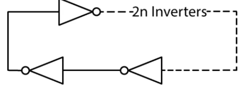
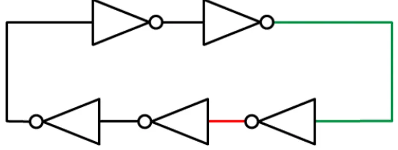
Ring oscillators are digital oscillators made of an odd number of inverters connected in a closed loop (fig. 3.1). These type of oscillators have plenty of advantages that make them interesting for our project: they are easily designed which CMOS technology, require a relatively low-voltage to achieve oscillatory behaviour and possess a wide tuning rage. [15]
Figure 3.1: Assembly of a ring oscillator, where n can be any natural number or zero.
The oscillation frequency (fo) of any RO depends on the delay of each stage and the
number of stages that comprised him.
C H A P T E R 3 . E L E M E N T S A N D P R O P O S E D I D E A
In order to understand it better one has to have in mind that every oscillator has a N number of stages, where N is an odd number, each stage provides a phase shift of π/N and the dc inversion provides the remaining phase shift of π.
This stages can be compromised of different elements, in our case we opted by using single ended inverters (fig. 3.2), sometimes resourcing to two-gate NANDs to use as enablers.
Figure 3.2: Design of an Inverter.
The oscillating signal has to go through each of the N delay stages once to allow for the first π phase shift in a time of N ∗ τd, where τd represents the time delay of each
inverter, and it must go through each stage a second time to allow for the 2π phase shift to be completed. So the frequency of oscillation (fo) is given by equation3.1.
fo=
1
2 ∗ N ∗ τd (3.1)
τdis defined as the time delay taken to reach the output voltage at 50% of its maximum value VDD [15].
In cases where the rise and fall times are different, given the values of τdhland τdlhas
the time taken for the signal to fall and rise, expression3.1can be rewritten to:
fo=
1
N ∗ (τdhl+ τdlh)
(3.2)
With all this in mind we have two options to easily change the fo, either change the size of the inverters or their number. Most authors usually recommend that the number of inverters is kept low or at a prime number in order to avoid the generation of higher harmonic signals [21] that can be mistaken by the fundamental frequency, obtaining the wrong propagation delay and hence, in our case, having a wrongful interpretation of the problem and its solution.
In regards to the power consumption of RO there are papers showing that it can be be decreased for oscillators in the range of the tens of MHz or less by using coupling and decreasing the channel width W to a minimum while enlarging the channel length L to obtain the desired frequency . We did not set any power requirements for this thesis, as
3 . 1 . E L E M E N T S U S E D
it pretends to be a mere proof of concept, and so our oscillators are done using the more traditional approach of using L minimum and using W and the number of inverters to set the frequency.
Besides the facts that [21] uses to discourage the use of an high number of inverters this method usually allows for sharp square wave signals as they tend to use the fastest inverters available for the technology.
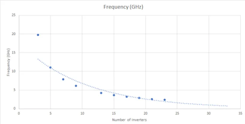
In order for us to have different frequencies we simply increase the number of invert-ers, we can see by the graphic in figure3.3that it has a significant impact on the frequency of the oscillators.
Figure 3.3: Frequency of oscillation based on the number of inverters at a fixed size.
Theoretically increasing the size of the transistors would also allow for slower oscil-lations, however we find it to not have such a strong effect and so opted out of it, and given the fact that the decrease in frequency has an exponential decay we could easily guarantee that we could create frequencies relatively small when compared to the ones produced by RO with only 3 or 5 inverters.
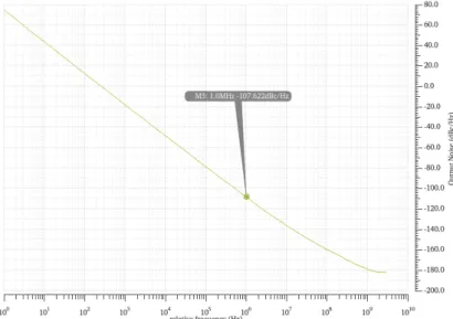
Ring oscillators tend to have a significant phase noise, however after analysing one of our ring oscillators (with the same size as before and with 23 stages) we can see in figure
3.4that they have a value of -107.622 dBc/Hz at 1MHz.
Given the fact that all the frequencies we will be testing in this cases are more than 1 MHz apart this should not be a problem. However the harmonics of some of the oscillators can in fact be a problem, and that is why we are implementing filters as can be read in section3.1.3.
3.1.2 Coupling of RO
The process of coupling ring oscillators is typically designed with the goal of achieving multiphase outputs, specially quadrature outputs as this cannot be achieved with single-ended inverters due to the fact that they require an odd (N ) number of inverters to work and so will only provide outputs with 2π/N phase deviation (as explained in section
3.1.1).
C H A P T E R 3 . E L E M E N T S A N D P R O P O S E D I D E A
Figure 3.4: Phase noise analysis of a RO.
The coupling of ring oscillators also helps with the low quality factor, Q, of ring oscillators as coupled ring oscillators tend to have a reduced single side band (SSB) phase noise [5] when compared to fully differential ring oscillators.
Another use of coupling in RO is to generate precise delays as it is shown by Maneatis and Horowitz [16].
The study of coupled ring oscillators is well documented for rings running at the same frequencies, or with harmonic frequencies that will eventually injection lock into a single frequency [8].
The design of a coupler is relatively simple and is, in general, done by shunting two inverters half the size of the ones normally used in the circuit, as it can be seen in figure
3.5.
Figure 3.5: Design of a coupler.
Our project on the other hand uses coupling with different size rings at different, and preferably non-harmonic, frequencies and focus mainly on the circuit transients. Leading to the fact very little literature is available to discuss the approaches taken on this thesis.
3 . 2 . P R O P O S E D I D E A
3.1.3 Filters
As stated before (in section3.1.1) Ring Oscillators tend to have a significant phase noise, this fortunately is not a problem that would interfere with our circuit, however the fact that some harmonic frequencies could frequency lock with the main frequencies of other oscillators lead us to the need of implementing some filtering in this project. Bandpass fil-ters can help to reduce this problem, ideally filfil-ters with a higher quality factor would lead to better results but in order to keep the design of the filters simple and their parameters easily calculated we used simple LC filters.
The equations for the LC can be easily deduced and we can achieve equation3.3for the central frequency.
ωo=√1
LC (3.3)
While the cutoff frequencies can be calculated with equation3.4.
ωc= ± 1 2RC + r ( 1 2RC) 2+ 1 LC (3.4)
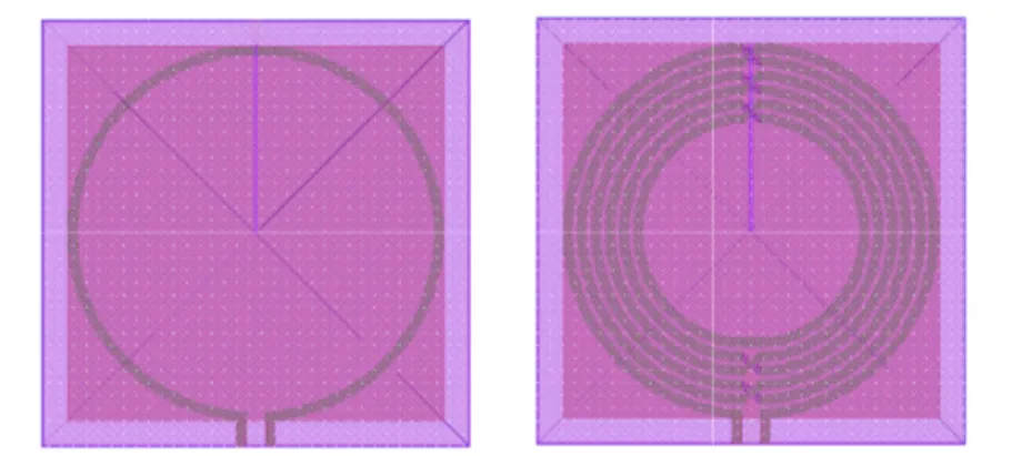
One of the problems with LC filters is that they use inductive elements, which is not something we would gladly put on any integrated circuit, in the future a different filter design could be used that would reduce the circuit area significantly. With the layout design in Cadences’ Virtuoso we could see that every inductor used in this project would be limited to an area of 170 sq.um. The edge cases of our application can be seen in figure
3.6.
Figure 3.6: Layout of UMC130nm inductors for our edge cases, to the left a 371pH inductor and to the right a 5.842nH inductor.
3.2
Proposed Idea
With the knowledge of the different elements done it is now time to understand how they can be combined to help solve the Travelling Salesman Problem. This next section is focused in detailing the idea behind the implementation while section4.1will explore
C H A P T E R 3 . E L E M E N T S A N D P R O P O S E D I D E A
said implementation deeper and at the same time address any improvements made to the original idea.
3.2.1 Working Principle
The TSP is characterised by two main thing: the number of cities and the distance between them.
Our idea consists of representing both the cities and the paths as Ring Oscillators. Where for each distance (or paths) we will have frequencies that can be connected to their respective cities by means of coupling.
By using RO to generate the frequencies (that represent each distance) we can couple their RO to both the ROs representing the Cities that this path connects. Allowing us to detect all the paths that are connected to one city by analysing the frequency spectrum of the respective RO.
Having in mind that higher frequencies means less stages, their signal should propa-gate faster, and so for our model to work it is important that the frequencies are correlated to the distances. In order to keep this standardised we initially opted by using a formula, where the number of inverters N would equal two times the distance d plus one, (equa-tion3.5), this would allow for an odd number of stages and give us a direct correlation between the distance and the frequencies .This was later changed in our implementation ,as we decided to fine tune the number of inverters in order to avoid having harmonic and sub-harmonic frequencies lock.
N = 2 ∗ d + 1 (3.5)
In our theory if all of the cities are connected, given enough time, we should be able to see all of the frequencies in all of the cities (as seen in figure3.7), indicating that there is some path that brings that determined frequency to our selected city. This obviously creates a problem with several path of the same distance in the circuit as that same frequency is repeated and so we might not be able to directly detect if a new path was followed, this problem was not address in this thesis.
To get the order that solves the TSP a disturbance would be made in the circuit, by either connecting or disconnecting a new city or injecting a new frequency in one of the cities (making this one the origin). There might be a need to inject the signal to see the outgoing path and turning off said signal to be able to see the incoming path computing all of the trajectory.
In the first part of the following chapter we will dive deeper into how this was imple-mented.
3 . 2 . P R O P O S E D I D E A
Figure 3.7: After some time we should be able to see all of the frequencies in all of the cities.
C
h
a
p
t
e
r
4
C i r c u i t I m p l e m e n ta t i o n a n d S i m u l a t i o n
R e s u lt s
With the information about most of the elements used in our implementation given in chapter3and a general idea of the principles behind our theory we will in this chapter first take a closer look into the implementation of the circuit (section4.1), look into how the tests where done (section 4.2) and finally some of the results that we were able to prove (section4.3).
All of the components were design using UMC 130nm CMOS technology and the simulations were done using Cadence Virtuoso.
4.1
Circuit Implementation
With the theoretical explanation done on section3.2we are now left with implementing it. We can divide the implementation in three different parts: Cities, Paths and Couplings. Each of this parts requires specific care that is detailed in the following sections.
4.1.1 Cities
Cities are responsible for showing what frequencies are coupled to them, with this in mind they are designed to have an oscillation frequency bigger than any of the paths that can lead to them and so they use transistors with small dimensions (the dimensions can be seen in table4.1) and a reduced number of inverters that allows for oscillation.
With only 5 inverters Cities are easily designed and run at a frequency of around 11GHz We can see in figure4.1what they look like, one of the branches would be used for the outgoing coupling followed, after one inverter, by the incoming coupling. This way everything that is going out will have passed through all the RO.
C H A P T E R 4 . C I R C U I T I M P L E M E N TAT I O N A N D S I M U L AT I O N R E S U LT S P-MOS N-MOS L 120nm 120nm W 30µm 10µm # Fingers 1 1 Multiplier 1 1
Table 4.1: Sizes used in the implementation of the cities’ inverters.
Figure 4.1: RO representing a city.
Due to the fact that we sometimes use LC filtering the inverters are design with supply voltages of 1.2V and −1.2V instead of the more traditional 1.2V and 0V .
In the rest of this chapter for any diagrams of circuits, tests, or other implementations we will use a letter within a circle to represent cities.
4.1.2 Paths
Paths are responsible for two main things: firstly they need to generate new frequencies that will represent the distance between the cities, and secondly they need to transport the frequencies that are already on the starting city to the following city.
The paths are also created using Ring Oscillators, this time we want them to run at significantly lower frequencies than the cities so we use a relatively higher number of inverters per RO as we have seen in figure3.3, the sizes used for the inverters can be seen in table4.2. P-MOS N-MOS L 120nm 120nm W 30µm 10µm # Fingers 1 1 Multiplier 5 5
Table 4.2: Sizes used in the implementation of the paths’ inverters.
As mentioned in section3.2.1we initially tried to follow equation3.5to define the number of inverters in a path, this led to some harmonic frequencies that would make the path or cities oscillators lock into a frequency destroying part of the information. We have since decided to use specific frequencies, even if this destroys the massification of this solution, in order to avoid frequency lock and make the proof of concept simpler.
4 . 1 . C I R C U I T I M P L E M E N TAT I O N
As with the cities the supply voltages of the inverters are of 1.2V and −1.2V , to allow for the use of LC band pass filtering, as seen in figure4.2.
Figure 4.2: Schematic of an inverter with voltage supply of 1.2V and −1.2V
In some of our testing one of the inverters is sometimes replaced with a two port NAND that will allow us to turn on and off the oscillations, there is a slight difference between the time taken by the NAND and the inverter to change state but as this change also changes the frequency of the overall oscillator our tests can be made the same just having in mind a different frequency for the filters.
After some ideas the RO were designed to represent bi-directional paths and so we split the number of inverters in half (with one extra one on one of the sides) and connected (coupled) each of the halves to a different city. This led to some complications with the frequencies so we set to start by only using uni-directional paths. In this cases the connection is made through a buffer (another inverter) that guarantees that the coupling is only made in one direction.
In the rest of this chapter for any diagram of circuits, tests, or other drawings we will use an arrow to represent a path, for each coloured arrow we can assume a different frequency and the arrow also points the direction of said path.
4.1.3 Coupling
There are two different connections that needed to be done for this project, the first one was the coupling of a path to a city and the second one the coupling of a city to a path, both of this connections are unidirectional and will only transmit information in one way.
4.1.3.1 Connecting a Path to a City
The connection from a Path to a City is created with a simple coupling, as stated in section
3.1.2usually the coupling of two ring oscillators is done with an element that shunts the output of two smaller inverters, in our case we opted by directly connecting the signal of the RO representing the path to an inverter to serve as a buffer and then directly to one of the branches of the RO representing the city.
C H A P T E R 4 . C I R C U I T I M P L E M E N TAT I O N A N D S I M U L AT I O N R E S U LT S
As we will be able to see in our testing (from section4.3onward) this coupling allows us to transmit the frequencies that are running through the path to a new city.
4.1.3.2 Connecting a City to a Path
For simple cases where only one or two paths are connected to a city a simple coupling like the one done when connecting a path to a city would suffice, however with an ever increasing number of frequencies showing up when the problem grows there is a need to add filters to cut part of the phase noise of the frequencies allowing for a cleaner result.
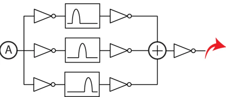
With that in mind when connecting a city to a path we first connect the outgoing signal to a inverter to work as a buffer followed by one or more filters (depending on the number of frequencies we want to isolate), the output of this filters goes through an inverter to serve as buffer and then goes through a summing amplifier and the signal is once again passed through an inverter before coupling. This final signal is connected to the following Path finishing the coupling. Figure4.3shows an example for a 3 frequency set up.
Figure 4.3: The coupling of a City to a Path with 3 different Bandpass Filters.
4.2
Methods of Analysis
As the core of the circuit works by analysing the spread of the different frequencies, most of the results come from analysing frequency spectra, this is usually done with the use of Fourier Transforms or automatically done with the help of the Fast Fourier Transform (FFT) [2]. As we want to see when each frequency starts to show up on the spectrum and which ones come first it is as important for us to have several FFTs as it is to know at what time intervals they were taken.
With this in mind we experimented with a method that we will call Time Swept FFT and that will produce a plethora of superimposed FFTs with a small increment in the starting time. Being the idea that we could analyse the behaviour of specific frequencies throughout time.
4 . 2 . M E T H O D S O F A N A LY S I S
4.2.1 Time Swept FFT
To apply our method we first create the simulation scenario on Cadence®and run a tran-sient simulation with a relatively small fixed step (around 1ps) and enough time to guar-antee stability (e.g. 500ns).
The transient signal is then exported to .csv file that is loaded into our MATLAB script (present in ANNEXI).
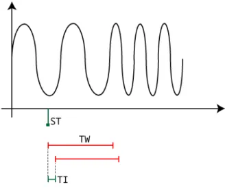
Besides the .csv file containing the timewave our script gets the following inputs:
• The starting time (ST) of the FFTs, as we sometimes want to wait some time for the circuit to get into a steady state before inserting a perturbation;
• The time window (TW) of the FFT, meaning of how many ns we want to make the FFT;
• The time increment (TI) that we want between the start of each FFT;
• The stopping time defined by the user.
Our script first detects the timestep used in the simulation as this is vital for the correct calculation of the FFT.
With the rest of the information already provided the script simply calculates the FFT, using the FFT implementation present in MATLAB, for a given time windows, appends the result to the CSV file, increases the starting time and then keeps this loop until we reach the stopping time. The figure4.4might help to better understand this method.
Figure 4.4: Schematic of how the Time Swept FFT works.
C H A P T E R 4 . C I R C U I T I M P L E M E N TAT I O N A N D S I M U L AT I O N R E S U LT S
4.3
Simulation Results
This section is focused in showing the results of the main simulations done while trying to prove possible the concept of calculating the solution for the Travelling Salesman Problem using a network of coupled ring oscillators. Unfortunately we unable to fully prove the concept during the writing of this thesis, so we set on writing about some landmark proofs: when we have several frequencies (paths) connecting to the same city, the fastest frequency (meaning the shortest distance) will reach the city first; If we have multiple frequencies arrived to a single city, one path leading out of that city is enough to carry all of them; The frequencies can be transported through several cities, spreading in the web of paths and cities.
4.3.1 Faster Frequencies Arrive Faster
The first one of our key points that needs proof is that when we have several frequencies (representing several paths) connected to the same oscillator (representing one city) the faster frequency would be the first to be detected on the oscillator, given the fact that all of them start at the same time, a simple scheme of the implementation can be seen in figure4.5.
Figure 4.5: For this test we have two different paths connected to one city.
To test this we created a scenario with two RO, running at two different frequencies (1.05GHz and 3.30GHz, representing two different paths) , connected to a third one running at a much higher frequency (11GHz, representing a city). A representation of the circuit can be seen in figure4.6.
In order to view which of the frequencies arrived first we took some precautions:
1. Each of the RO has a switch that will turn the middle oscillator on, allowing for the circuit to be closed and the oscillations to start, as seen in figure4.6;
2. The connection between the RO representing each path and the RO representing the city is also cut off with a switch inverter that will only turn on when the path oscillator is turned on, to allow for the oscillator representing the city to start to oscillate naturally.
Our test consisted on the following:
1. Starting the RO representing the City;
4 . 3 . S I M U L AT I O N R E S U LT S
Figure 4.6: Circuit with 2 RO, representing two paths, coupled to the same city.
2. Switch on all the switches, turning on the remaining oscillators (the paths) and connecting them to the the City;
3. Analyse the evolution of the FFT on the RO that represents the city using the method described on section4.2.1.
We analyse FFTs of 20ns time chunks and then increment the starting time by 0.2ns, this allows us to have enough resolution in the spectrum and at the same time denote at what time the new frequencies start to emerge.
By creating a superposition of the different FFTs we can see the rise of the Paths’ frequencies as the time goes by .
The most complicated part in this analysis is to know which of the frequencies can be accepted as arriving before. As both of the frequencies will rise to different values we cannot simply decide a threshold value and signal which of the frequencies arrives there first.
In order to prove that in fact higher frequencies can be detected before slower fre-quencies we let the circuit stabilise first and averaged the last 5 values of the FFT in those frequencies. We then created a table (table4.3) of that average value, 20% of it and 50% of it for each of the frequencies.
With this in mind we looked in our Time Swept FFT for those values of 20% and 50% of the average after stabilisation and we can see that higher frequencies will arrive at those values first.
Table 4.3: Average values measured on the FFT for each signal.
Frequency Average 5 0.2 * Avg 5 0.5 * Avg 5 1.05 GHz 0.604126 0.1208252 0.302063 3.30 GHz 0.683162 0.1366324 0.341581
When comparing the values of table4.3to the values given by the different FFTs we created table4.4where the yellow cells represent values above the 20%Avg5. We can see
that the highest frequency arrives at least 0.4ns before the other one.
C H A P T E R 4 . C I R C U I T I M P L E M E N TAT I O N A N D S I M U L AT I O N R E S U LT S
Table 4.4: Analysis of our TimeSwept FFT with 20 ns windows starting from 13.4ns to 14.4ns. Frequency Starting Time 13.4ns 13.6ns 13.8ns 14.0ns 14.2ns 14.4ns 1.05 GHz 0.10297 0.099594 0.11116 0.1119 0.12218 0.13305 3.30 GHz 0.13045 0.13444 0.14096 0.14576 0.15029 0.15156
When analysing for the 50%Avg5we see the time difference increase to at least 0.8ns,
this results can be seen in table4.5.
Table 4.5: Analysis of our TimeSwept FFT with 20 ns windows starting from 19ns to 20ns.
Frequency
Starting
Time 19ns 19.2ns 19.4ns 19.6ns 19.8ns 20ns
1.05 GHz 0.27202 0.28501 0.28404 0.29501 0.29661 0.30911 3.30 GHz 0.33996 0.35052 0.35139 0.36242 0.36248 0.37279
This results are unfortunately dependent of knowing the value at which the signal stabilises. We could, in theory, use a set threshold value but for now we have no way of knowing if that would lead to a correct extrapolation of the order by which the frequencies arrive. Despite the fact that this method seemed to work for this, and other tested cases, there is no proof was made that it is valid for every iteraction of the problem and some more in depth testing should be done.
4.3.2 The circuit redirects multiple frequencies
The second key point that required some proof was that a City after receiving informa-tion from several Paths could in fact transfer all of that informainforma-tion to the following city through each path. In order to test this hypothesis we used the circuit from subsec-tion4.3.1and added a new path leading to a new RO that represents a second city, the representation of this scenario can be seen in figure4.7.
Figure 4.7: Representation of the test assembled to test this scenario.
To help keep track of the frequencies table4.6was created.
In this case the test is simpler than the one on the section4.3.1as we are not looking into any time dependence we simply ran the circuit (fig. 4.8) with the Blue and Green
4 . 3 . S I M U L AT I O N R E S U LT S
Table 4.6: Frequency of the different Paths used on test number 2. Colour Frequency Origin Destination
Blue 1.05 GHz - City A
Green 3.3 GHz - City A
Red 2.0 GHz City A City B
paths turned off until stabilisation and then proceeded to turn on those two paths to see the new stripes show up on our FFT.
Figure 4.8: Circuit with 2 RO, representing two paths, connected to the same city and then a third path connecting to another city.
By analysing the FFTs before and after turning on the RO of the paths (figure4.9we can see two new spikes related to the frequencies of 1.05GHz and 3.30GHz. There is also a small frequency shift for the remaining frequency (2GHz) that has probably locked in with one of harmonics of one of the 1.05GHz frequency.
Figure 4.9: Superposition of an FFT before and after turning on the first two paths.
We can assume that the frequencies, in this case at least, are in fact redirected from City A to City B. It is also important to note that from the two frequencies redirected from City A to City B one of them is a lower frequency than the one from the path that makes the connection and the other one is an higher frequency.
C H A P T E R 4 . C I R C U I T I M P L E M E N TAT I O N A N D S I M U L AT I O N R E S U LT S
4.3.3 The Frequencies are passed from city to city
The final point we felt like needed to be addressed is the fact that this frequencies need to pass through several cities without a major loss of amplitude, otherwise there would be no way of knowing if X City has already passed.
With this in mind we assembled a relatively simple test with 3 cities only connected with one path between each of them (as seen in figure4.10with the goal of looking into the last city and seeing if all of the frequencies were detected.
Figure 4.10: Representation of the test assembled to test this scenario.
Similarly to the test done on section4.3.2we were only interested in the frequency domain and so we waited for the circuit to stabilise before obtaining the FFT (figure4.11
where we looked for the frequencies on table4.7.
Table 4.7: Frequency of the different Paths used on test number 3. Colour Frequency Origin Destination
Blue 3.75 GHz - City A
Red 1.85 GHz City A City B Orange 950 MHz City B City C
Observing figure4.11we can see three main stripes corresponding to the frequencies of the three paths and so we can assume that the frequencies in fact tend to travel through the circuit, it is interesting to note that looking at this example the amplitude of the frequency stripes does not seem to be related to the distance travelled by the signal as the amplitude of the 3.75GHz stripe is similar to the amplitude of the 1, 85GHz stripe.
It is also interesting to note that this was the only test where we used the filters, as the noise produced from the consecutive coupling would ruin the reading. This might be one of the reasons for the frequencies to not degradate as fast as we have filtered out some of the noise in every coupling.
4 . 3 . S I M U L AT I O N R E S U LT S
Figure 4.11: FFT on City C after the circuit stabilised.
C
h
a
p
t
e
r
5
C o n c lu s i o n s a n d F u t u r e Wo r k
5.1
Conclusions
As seen in Chapter2The Travelling Salesman Problem is a NP hard problem that has been one of the landmarks to prove the advantages of new computational methods against classical computation.
We thought of a way to make quantum-like computation using a standard CMOS technology by implementing a circuit that would emulate the Travelling Salesman Prob-lem and let us compute its solution by analysing the frequency spectra of one or several points of the circuit. The implementation ended up, similarly to the initial idea, being composed by several ring oscillators (as studied in Chapter3) coupled together. Some design changes were made to help avoid frequency lock and streamline the overall results, while others were made in order to correct the initial idea that would not emulate the problem properly.
The initial goal started with the 5 City TSP initially shown in figure1.1. We improved the design in order to have the frequency of the "City"oscillator significantly higher than the frequency of the oscillators of the "Paths"but still some complications started to show when trying to solve it straight away and there was a decision to decrease the goal to a 3 City 4 Path TSP like the one shown in figure1.2. Even with this alteration some prob-lems showed up with the paths leading back to the same city creating some unexpected behaviours.
A decision was then made to try to focus in testing small parts of the circuit and build from there, this part is shown in Chapter4where we prove 3 main points:
1. Following our heuristic (section ??) higher frequencies will express themselves ear-lier, when coupled to the same oscillator;
C H A P T E R 5 . C O N C LU S I O N S A N D F U T U R E WO R K
2. One RO can "transport"several frequencies;
3. This frequencies can be passed through an array of oscillators without major de-creases in amplitude.
These three points are founding blocks for what can be a simple CMOS implementable circuit to solve a NP-hard problem like the TSP. While unfortunately the conclusions of this thesis are not as much of a breakthrough as initially thought they can be a small stepping stone for future projects.
However there are still two points that would require special attention: first there is a need to prove that the tests done here in small examples could be expanded to larger scenarios and secondly we need to make sure that the filters are in fact filtering important information from the noise and not only keeping part of the noise. With this taken care of we could work on some future implementations.
5.2
Future Work
As this thesis ended up not reaching the goal of solving a simple TSP, and in order for that to be possible, there are some steps to be made:
1. Understand the behaviour of the circuit with paths that come back to the starting cities, as during our tests they have brought to the system some instability and noise that deemed the reading of the solution impossibly hard;
2. Having encoded the full TSP the methodology to get back the answer might need some adjustments as our idea was not tested.
Given some time to ths ideas we should be able to solve the TSP using Ring Oscillators.
B i b l i o g r a p h y
[1] S. Boixo, V. N. Smelyanskiy, A. Shabani, S. V. Isakov, M. Dykman, V. S. Denchev, M. H. Amin, A. Y. Smirnov, M. Mohseni, and H. Neven. “Computational multiqubit tunnelling in programmable quantum annealers.” In: Nature Communications 7
(2016), p. 10327. d o i:10.1038/ncomms10327.
[2] E. O. Brigham and R. E. Morrow. “The fast Fourier transform.” In: IEEE Spectrum
4.12 (1967), pp. 63–70. i s s n: 0018-9235. d o i:10.1109/MSPEC.1967.5217220. [3] S. G. BRUSH. “History of the Lenz-Ising Model.” In: Rev. Mod. Phys. 39 (4 1967),
pp. 883–893. d o i: 10.1103/RevModPhys.39.883.
[4] G. Csaba, A. Raychowdhury, S. Datta, and W. Porod. “Computing with Coupled Oscillators: Theory, Devices, and Applications.” In: 2018 IEEE International
Sym-posium on Circuits and Systems (ISCAS). 2018, pp. 1–5. d o i: 10.1109/ISCAS.2018.
8351664.
[5] L. Dai and R. Harjani. “Analysis and design of low-phase-noise ring oscillators.” In:
Proceedings of the 2000 international symposium on Low power electronics and design - ISLPED ’00. l. New York, New York, USA: ACM Press, 2000, pp. 289–294. i s b n:
1581131909. d o i: 10 . 1145 / 344166 . 344639. u r l: http : / / portal . acm . org / citation.cfm?doid=344166.344639.
[6] S. Datta, N. Shukla, M. Cotter, A. Parihar, and A. Raychowdhury. “Neuro inspired computing with coupled relaxation oscillators.” In: 2014 51st ACM/EDAC/IEEE
Design Automation Conference (DAC). 2014, pp. 1–6. d o i: 10 . 1145 / 2593069 .
2596685.
[7] V. S. Denchev, S. Boixo, S. V. Isakov, N. Ding, R. Babbush, V. Smelyanskiy, J. Marti-nis, and H. Neven. “What is the Computational Value of Finite-Range Tunneling?”
In:Physical Review X 6.3 (2016). d o i: 10.1103/physrevx.6.031015.
[8] I. Dubey Prashant (Greater Noida. “Coupled ring oscillator.” Pat. 8638175. 2014. u r l:http://www.freepatentsonline.com/8638175.html.
[9] A. Finnila, M. Gomez, C. Sebenik, C. Stenson, and J. Doll. “Quantum annealing: A new method for minimizing multidimensional functions.” In:Chemical Physics
Letters 219.5–6 (1994), 343–348. d o i: 10.1016/0009-2614(94)00117-0.
B I B L I O G R A P H Y
[10] S. V. Isakov, G. Mazzola, V. N. Smelyanskiy, Z. Jiang, S. Boixo, H. Neven, and M. Troyer. “Understanding Quantum Tunneling through Quantum Monte Carlo Simulations.” In: Physical Review Letters 117.18, 180402 (2016), p. 180402. d o i:
10.1103/PhysRevLett.117.180402. arXiv:1510.08057 [quant-ph].
[11] T. S. Jordan, S. Scott, D. Leonhardt, J. O. Custer, C. T. Rodenbeck, S. Wolfley, and C. D. Nordquist. “Model and characterization of VO2 thin-film switching devices.”
In:IEEE Transactions on Electron Devices 61.3 (2014), pp. 813–819. issn: 00189383.
d o i:10.1109/TED.2014.2299549.
[12] M. Jünger, G. Reinelt, and G. Rinaldi. “Chapter 4 The traveling salesman prob-lem.” In: Handbooks in Operations Research and Management Science. Elsevier, 1995,
225–330. d o i: 10.1016/s0927-0507(05)80121-5.
[13] S. Kirkpatrick, C. D. Gelatt, and M. P. Vecchi. “Optimization by simulated anneal-ing.” In: Science 220 4598 (1983), pp. 671–80.
[14] N. Locatelli, V. Cros, and J. Grollier. “Spin-torque building blocks.” In: Nature
Materials 13.1 (2014), pp. 11–20. i s s n: 14764660. d o i: 10.1038/nmat3823. u r l:
http://dx.doi.org/10.1038/nmat3823.
[15] M. K. Mandal and B. C. Sarkar. “Ring oscillators : Characteristics and applications.” In: 2010.
[16] J. G. Maneatis and M. A. Horowitz. “Precise delay generation using coupled oscil-lators.” In: IEEE Journal of Solid-State Circuits 28.12 (1993), pp. 1273–1282. i s s n:
0018-9200. d o i:10.1109/4.262000.
[17] N. Metropolis, A. W. Rosenbluth, M. N. Rosenbluth, A. H. Teller, and E. Teller. “Equation of State Calculations by Fast Computing Machines.” In: 21 (June 1953),
pp. 1087–1092. d o i: 10.1063/1.1699114.
[18] A. Parihar, N. Shukla, S. Datta, and A. Raychowdhury. “Exploiting synchronization properties of correlated electron devices in a non-boolean computing fabric for template matching.” In: IEEE Journal on Emerging and Selected Topics in Circuits and
Systems 4.4 (2014), pp. 450–459. i s s n: 21563357. d o i: 10.1109/JETCAS.2014.
2361069.
[19] M. R. Pufall, W. H. Rippard, S. Kaka, T. J. Silva, and S. E. Russek. “Frequency modulation of spin-transfer oscillators.” In: Applied Physics Letters 86.8 (2005),
pp. 1–3. i s s n: 00036951. d o i:10.1063/1.1875762.
[20] A. Raychowdhury, A. Parihar, G. H. Smith, V. Narayanan, G. Csaba, M. Jerry, W. Porod, and S. Datta. “Computing With Networks of Oscillatory Dynamical Systems.” In: Proceedings of the IEEE 107.1 (2019), pp. 73–89. i s s n: 0018-9219.
d o i:10.1109/JPROC.2018.2878854.