8-Phase Ring Oscillator for Modern Receivers

Ricardo Filipe Malaia Neves

Licenciado em Ciências da Engenharia Electrotécnica

e de Computadores

8-Phase Ring Oscillator for Modern Receivers

Dissertação para obtenção do Grau de Mestre em

Engenharia Electrotécnica e de Computadores

Orientador: Luís Augusto Bica Gomes de Oliveira, Prof. Auxiliar, Universidade Nova de Lisboa

Júri:

Presidente: . .

Arguentes:

8-Phase Ring Oscillator for Modern Receivers

Copyright © Ricardo Filipe Malaia Neves, Faculdade de Ciências e Tecnologia, Universidade Nova de Lisboa.

Agradecimentos

É devido a uma sensação de enorme gratidão para com certas pessoas que, quer já trouxesse no coração, quer tenha conhecido durante todos estes anos de conquistas, tenho de fazer alguns agradecimentos.

Em primeiro lugar, reconhecer que a FCT-UNL é uma mais-valia como instituição de ensino superior. Instituição essa que me concedeu a extraordinária oportunidade de conhecer e trabalhar com alguns professores verdadeiramente notáveis nas suas respectivas áreas.

Professores como João Goes, que foi o responsável pelo início da minha paixão pela Microelectrónica, passando pelos professores Luís Gomes e Anikó Costa por terem depositado em mim toda a sua compreensão e fé em tempos mais difíceis e, como seria óbvio, pelo meu orientador Prof. Luís Oliveira, pela sua dedicação enquanto professor, e agora poderia ficar a escrever durante horas que nunca conseguiria descrever a real importância que o professor teve, tanto a nível académico como pessoal, na minha vida. Agradeço assim a todos eles por terem tido um papel relevante no meu percurso académico.

Em segundo lugar gostaria de reconhecer a importância de alguns colegas e amigos. Colegas como Ivan Bastos e Edinei Santin que sem os quais este documento não teria o valor que tem. Amigos como o Carlos Carvalho, Manuel Gomes, João Matos, Ali Saad e o meu amigo

de infância Tiago Silva, que me ajudaram a crescer e fizeram valer a pena cada “baixo” que encontrei no meu percurso durante estes anos, porque eles mesmos foram os “altos” que anularam os “baixos”. O meu muito obrigado por serem quem são.

Ainda assim gostaria de relevar e destacar de uma forma muito clara, dois amigos em particular que, contribuíram decisivamente, para que esta meta final se tornasse uma realidade. São eles o Pedro Dias e o Luís Neto.

Queria também agradecer a toda a minha família incluindo àqueles que já cá não estão por me terem podido colocar o pão na minha mesa durante a minha vida inteira e porque sem eles eu nunca teria passado pelos melhores anos que se pode viver, os anos de faculdade.

Abstract

The evolution of receiver architectures, built in modern CMOS technologies, allows the design of high efficient receivers. A key block in modern receivers is the oscillator. The main objective of this thesis is to design a very low power and low area 8-Phase Ring Oscillator for biomedical applications (ISM and WMTS bands).

Oscillators with multiphase outputs and variable duty cycles are required. In this thesis we are focused in 12.5% and 50% duty-cycles approaches. The proposed circuit uses eight inverters in a ring structure, in order to generate the output duty cycle of 50%. The duty cycle of 1/8 is achieved through the combination of the longer duty cycle signals in pairs, using, for this purpose, NAND gates. Since the general application are not only the wireless communications context, as well as industrial, scientific and medical plans, the 8-Phase Oscillator is simulated to be wideband between 100 MHz and 1 GHz, and be able to operate in the ISM bands (447 MHz-930 MHz) and WMTS (600 MHz).

The circuit prototype is designed in UMC 130 nm CMOS technology. The maximum value of current drawn from a DC power source of 1.2 V, at a maximum frequency of 930 MHz achieved, is 17.54 mA. After completion of the oscillator layout studied (occupied area is 165

μm x 83μm). Measurement results confirm the expected operating range from the simulations, and therefore, that the oscillator fulfil effectively the goals initially proposed in order to be used as Local Oscillator in RF Modern Receivers.

Resumo

A evolução das arquitecturas de receptores, construídos através de tecnologias modernas CMOS, permite o dimensionamento de receptores altamente eficientes. Um bloco importante nos receptores modernos é o oscilador. O principal objectivo desta dissertação, passa pelo estudo de um Oscilador em Anel de 8 Fases de área e consumo muito reduzidos, para uso em aplicações biomédicas (bandas ISM e WMTS).

São cada vez mais necessários, osciladores capazes de fornecer variadas fases e fabricar diferentes duty cycles. Nesta tese o foco encontra-se em aproximações com duty cycles de 12.5% e 50%. O circuito apresentado utiliza 8 inversores em formação de anel, de forma a gerar os duty cycles de 50%. O duty cycle de 1/8 é alcançado através da combinação dos sinais já existentes, dois a dois, nas entradas de uma porta lógica NAND. Tendo em conta que o Oscilador de 8 Fases não é projectado apenas com vista a comunicações sem fios, mas também com vista os planos industriais, científicos e médicos, o Oscilador de 8 Fases é simulado de forma obter uma largura de banda entre os 100 MHz e 1 GHz, e ser capaz de funcionar dentro das bandas ISM (447 MHz-930 MHz) e WMTS (600 MHz).

O circuito protótipo é implementado numa tecnologia UMC 130 nm CMOS. A corrente máxima, fornecida pela fonte de tensão DC de 1,2 V, alcançada a uma frequência de oscilação de 930 MHz, é 17,54 mA. Após a conclusão do layout do oscilador em estudo (área ocupada de 165 μm x 83μm), resultados das medições confirmam a banda de funcionamento prevista pelas

simulações e, também, que o oscilador cumpre de forma eficaz todas as metas propostas inicialmente com a finalidade de ser utilizado em Receptores RF Modernos como Oscilador Local.

Palavras-chave:“Layout”, Inversores CMOS, Oscilador em anel, Oscilador de várias fases,

Abbreviations

ADC Analog-To-Digital Converter

CMOS Complementary Metal-Oxide-Semiconductor

DC Direct Current

DT Discrete-Time

HR Harmonic-Rejection

IF Intermediate Frequency

IIP Intermodulation Intercept Point IIR Infinite Impulse Response ISM Industrial, Scientific and Medical LNA Low Noise Amplifier

LO Local Oscillator

NF Noise Figure

NMOS Nchannel Metal-Oxide-Semiconductor PLL Phase Locked Loop

PMOS Pchannel Metal-Oxide-Semiconductor

RF Radio Frequency

SC Switched-Capacitor

VCO Voltage-Controlled Oscillator WMTS Wireless Medical Telemetry Service LPF Low Pass Filter

Contents

1 INTRODUCTION ... 1

1.1 BACKGROUND AND MOTIVATION ... 1

1.2 THESIS ORGANIZATION ... 2

1.3 MAIN CONTRIBUTIONS ... 3

2 RECEIVER ARCHITECTURES AND RF BLOCKS ... 5

2.1 RECEIVER ARCHITECTURES ... 5

2.1.1 Heterodyne or IF Receivers ... 6

2.1.2 Homodyne or Zero-IF Receivers ... 7

2.1.3 Low-IF Receivers ... 9

2.2 LNABASIC CONCEPTS ... 11

2.2.1 S-Parameters ... 11

2.2.2 Stability ... 12

2.2.3 Noise Figure ... 13

2.3 MIXERS ... 14

2.3.1 Performance Parameters of Mixers ... 15

2.3.2 Different Types of Mixers ... 17

3 OSCILLATORS ...21

3.1 BARKHAUSEN CRITERION ... 21

3.2 PHASE-NOISE ... 22

3.3 QUALITY FACTOR ... 24

3.4 EXAMPLES OF OSCILLATORS ... 26

3.4.1 LC Oscillator ... 26

3.4.2 Relaxation Oscillators ... 27

3.4.3 Coupled Ring Oscillators ... 28

4 8 PHASES OSCILLATOR ...33

4.1 INTRODUCTION ... 33

4.2 DOWNCONVERTER ARCHITECTURE ... 34

4.3 CIRCUIT BLOCKS:SAMPLING CELL AND LOCAL OSCILLATOR ... 35

4.3.1 Sampling/IIR filter cell ... 35

4.3.2 The Local Oscillator ... 36

4.4 8PHASES OSCILLATOR ARCHITECTURE ... 38

xvi

4.5.1 Inverters ... 40

4.5.2 Buffer ... 41

4.5.3 AND ... 42

4.5.4 Current Mirrors ... 44

5 SIMULATION AND MEASUREMENT RESULTS ...47

5.1 SCHEMATIC SIMULATIONS ... 47

5.1.1 12.5 % Duty Cycle ... 49

5.1.2 50 % Duty Cycle ... 51

5.1.3 Phase Noise ... 53

5.2 LAYOUT ... 53

5.3 POST-LAYOUT SIMULATIONS ... 56

5.3.1 12.5 % Duty Cycle ... 58

5.3.2 50 % Duty Cycle ... 59

5.3.3 Phase Noise ... 60

5.3.4 Schematic vs. Post-Layout Simulations ... 61

5.4 MEASUREMENT RESULTS ... 62

6 CONCLUSIONS AND FUTURE WORK ...65

6.1 CONCLUSIONS ... 65

6.2 FUTURE WORK ... 66

List of Figures

FIGURE 2-1–BASIC HETERODYNE ARCHITECTURE [1]. ... 6

FIGURE 2-2–IMAGE REJECTION FUNDAMENTALS [13]. ... 7

FIGURE 2-3–BASIC HOMODYNE ARCHITECTURE [1]. ... 8

FIGURE 2-4–HARTLEY ARCHITECTURE [1]. ... 10

FIGURE 2-5–WEAVER ARCHITECTURE [1]. ... 10

FIGURE 2-6–S-PARAMETERS [16]. ... 12

FIGURE 2-7–NOISE NETWORK [16]. ... 13

FIGURE 2-8–NOISE NETWORK [2]. ... 14

FIGURE 2-9–MIXING OPERATION. ... 15

FIGURE 2-10–DOWN-CONVERSION RESULTING SPECTRUM. ... 15

FIGURE 2-11–3RD_O RDER INTERCEPT POINT (IIP3). ... 17

FIGURE 2-12–PASSIVE MIXER USING ACTIVE DEVICE [2]. ... 18

FIGURE 2-13–SINGLE BALANCED MIXER [1]. ... 19

FIGURE 2-14–GILBERT CELL. ... 20

FIGURE 3-1–SIMPLE FEEDBACK SYSTEM [1]. ... 22

FIGURE 3-2–IDEAL CARRIER AND CARRIER WITH PHASE-NOISE (ADOPTED FROM [17]). ... 23

FIGURE 3-3–PHASE-NOISE EFFECT IN DOWN-CONVERSION (ADOPTED FROM [17]). ... 23

FIGURE 3-4–PHASE-NOISE SINGLE SIDE BAND (ADOPTED FROM [17]). ... 24

FIGURE 3-5–CARRIER SPECTRUM REGARDING VARIATIONS IN THE QUALITY FACTOR. ... 24

FIGURE 3-6–LCOSCILLATOR [1]. ... 26

FIGURE 3-7–LCOSCILLATOR LINEAR MODEL. ... 27

FIGURE 3-8–RELAXATION OSCILLATOR [1]. ... 28

FIGURE 3-9–3-STAGE SINGLE-ENDED RING OSCILLATOR. ... 28

FIGURE 3-10–TWO SETS OF 3-STAGE RING OSCILLATORS COUPLED TOGETHER [20]. ... 29

FIGURE 3-11–QUADRATURE FOUR-STAGE RING OSCILLATOR [34]. ... 30

FIGURE 3-12–TWO DIMENSIONAL ARRAY OSCILLATOR [20]. ... 31

FIGURE 4-1–BLOCK DIAGRAM OF THE IMPLEMENTED DT MIXING CIRCUIT COMPRISING THE INPUT DRIVER,SC DOWNCONVERTER CORE AND THE LO(ADOPTED FROM [11]). ... 34

FIGURE 4-2–SC CORE OF THE DOWNCONVERTER (ADOPTED FROM [11]). ... 35

FIGURE 4-3– A)SCHEMATIC OF A SU; B)MOS CAPS WITH EMBEDDED PA(ADOPTED FROM [11]). ... 35

FIGURE 4-4–(A)LOCAL OSCILLATOR;(B)8-PHASE 12.5%-DUTY-CYCLE WAVE FORMS. ... 36

FIGURE 4-5–NAND GATE SCHEMATIC. ... 37

FIGURE 4-6–TRANSFORMATION OF 12,5% TO 50% DUTY CYCLE WAVE. ... 38

xviii

FIGURE 4-8–INVERTER BLOCK SCHEMATIC. ... 40

FIGURE 4-9–BUFFER BLOCK SCHEMATIC. ... 41

FIGURE 4-10–AND BLOCK SCHEMATIC. ... 43

FIGURE 4-11–PMOSCURRENT MIRROR BLOCK SCHEMATIC. ... 44

FIGURE 4-12–NMOSCURRENT MIRROR BLOCK SCHEMATIC. ... 45

FIGURE 5-1–SCHEMATIC SEQUENTIAL SIGNALS WITH DUTY CYCLE OF 12.5%. ... 48

FIGURE 5-2–SCHEMATIC SEQUENTIAL SIGNALS WITH DUTY CYCLE OF 50%. ... 48

FIGURE 5-3–SCHEMATIC SIMULATIONS OF THE SIGNALS WITH DUTY CYCLE OF 12.5% AT 900MHZ, IN-PHASE AND IN PHASE INVERSION. ... 49

FIGURE 5-4–SCHEMATIC SIMULATIONS OF THE SIGNALS WITH DUTY CYCLE OF 12.5% AT 600MHZ, IN-PHASE AND IN PHASE INVERSION. ... 50

FIGURE 5-5–SCHEMATIC SIMULATIONS OF THE SIGNALS WITH DUTY CYCLE OF 12.5% AT 400MHZ, IN-PHASE AND IN PHASE INVERSION. ... 50

FIGURE 5-6–SCHEMATIC SIMULATIONS OF THE SIGNALS WITH DUTY CYCLE OF 50% AT 900MHZ, IN-PHASE AND IN PHASE INVERSION. ... 52

FIGURE 5-7–SCHEMATIC SIMULATIONS OF THE SIGNALS WITH DUTY CYCLE OF 50% AT 600MHZ, IN-PHASE AND IN PHASE INVERSION. ... 52

FIGURE 5-8–SCHEMATIC SIMULATIONS OF THE SIGNALS WITH DUTY CYCLE OF 50% AT 400MHZ, IN-PHASE AND IN PHASE INVERSION. ... 52

FIGURA 5-9PHASE NOISE OF THE OSCILLATOR AT 900MHZ OSCILLATING FREQUENCY. ... 53

FIGURE 5-10–CURRENT MIRROR LAYOUT. ... 54

FIGURE 5-11–NAND LAYOUT. ... 54

FIGURE 5-12–BUFFERS LAYOUT. ... 54

FIGURE 5-13–INVERTERS LAYOUT. ... 54

FIGURE 5-14–LAYOUT OF THE 8-PHASES RING OSCILLATOR (165 X 83 µM2). ... 55

FIGURE 5-15–CALIBRE SEQUENTIAL SIGNALS WITH DUTY CYCLE OF 12.5%. ... 56

FIGURE 5-16–CALIBRE SEQUENTIAL SIGNALS WITH DUTY CYCLE OF 50%. ... 57

FIGURE 5-17–CALIBRE SIMULATIONS OF THE SIGNALS WITH DUTY CYCLE OF 12.5% AT 900MHZ, IN-PHASE AND IN PHASE INVERSION. ... 58

FIGURE 5-18–CALIBRE SIMULATIONS OF THE SIGNALS WITH DUTY CYCLE OF 12.5% AT 600MHZ, IN-PHASE AND IN PHASE INVERSION. ... 58

FIGURE 5-19–CALIBRE SIMULATIONS OF THE SIGNALS WITH DUTY CYCLE OF 12.5% AT 400MHZ, IN-PHASE AND IN PHASE INVERSION. ... 58

FIGURE 5-20–CALIBRE SIMULATIONS OF THE SIGNALS WITH DUTY CYCLE OF 50% AT 900MHZ, IN-PHASE AND IN PHASE INVERSION. ... 59

FIGURE 5-21–CALIBRE SIMULATIONS OF THE SIGNALS WITH DUTY CYCLE OF 50% AT 600MHZ, IN-PHASE AND IN PHASE INVERSION. ... 59

FIGURE 5-22–CALIBRE SIMULATIONS OF THE SIGNALS WITH DUTY CYCLE OF 50% AT 400MHZ, IN-PHASE AND IN PHASE INVERSION. ... 59

FIGURE 5-23-PHASE NOISE OF THE OSCILLATOR AT 900MHZ OSCILLATING FREQUENCY. ... 60

FIGURE 5-25–LAYOUT OF THE FRONT-END WITH THE LNA WITH ACTIVE LOADS (800 X 550 µM2). ... 62

FIGURE 5-26–DIE PHOTO OF THE FRONT-END WITH THE LNA WITH ACTIVE LOADS (800 X 550 µM2). ... 63

FIGURE 5-27–PROTOTYPE BOARD (ADOPTED FROM [12]). ... 63

List of Tables

TABLE 4.1–TRUTH TABLE OF A NAND GATE. ... 38

1

Introduction

1.1

Background and Motivation

Modern transceivers for wireless communications require circuits with low power consumption, size, cost, noise, while increasing the frequency and bandwidth. The successful travel of wireless communications led to new and more challenging requirements such as: low supply voltage, low cost, and low area circuits. The use of modern CMOS nanotechnologies allows, by adjusting old architectures or by employing new circuit designs, to find a way to reach these objectives [1].

The circuit between the antenna and the digital part, is generally defined as the RF front-end. Due to very tough specifications for RF blocks, the receiver front-end has a very important role in communications. Receiver architectures can be divided into: heterodyne and homodyne. The first converts the signal to an intermediate frequency (IF), while the second downconverts directly to the baseband. Combining the main advantages of both architectures, the Low-IF receiver is a modified version of the homodyne and is becoming a good alternative [1, 2].

Due to development of wireless receiver architectures, image-rejection topologies require accurate quadrature voltage-controlled oscillator (VCO). The way to keep an oscillator outputs stable in frequency and phase, is to connect two oscillators in a feedback structure, in order to be able to generate signals with a precise 90° phase shift. There’s many ways to obtain accurate quadrature outputs. Due to this, new architectures have emerged using RC and LC oscillators, some of them have inherent quadrature outputs, for example the two integrator oscillator [1].

On the other hand, oscillators with wide operating range, they can provide different carrier frequencies and data rates for wireless transmissions in the existing variety of

2

communication standards. A polyphase filter can produce quadrature signals using differential outputs of a VCO [3], [4]. Another technique to get quadrature output is to design a VCO, which works at double the desired frequency, followed by frequency division [5]. Coupled VCOs structure [6] and [7], coupled resonators in a ring structure [8], and multiphase ring oscillators [9] are other alternatives to produce quadrature outputs [10]. The architecture proposed in this thesis uses a combination of cross-coupled inverters and ring oscillators concept, for generating multiphase outputs.

1.2

Thesis Organization

This thesis is presented into six chapters, including the present introduction. Since each chapter begins with a small introduction presenting that specific topics, here it is just a brief and general reference to each chapter.

Chapter 2 - Receiver Architectures and RF Blocks: this chapter is the literature review of the dissertation, introducing and describing the main architectures related to both receivers and the RF blocks.

Chapter 3 - Oscillators: is hereby continued the previous chapter, but with a more detailed view only on the RF block in which this thesis focuses properly. It is also included, in the final part, the chosen architecture for the oscillator design.

Chapter 4 - 8 Phases Oscillator: is dedicated to the context of the proposed circuit, that is, will be presented the actual topology where the oscillator in study came from. Following that first half, a more detailed study of the proposed topology and sizing of the projected oscillator and its most intimate blocks will also be presented.

Chapter 5 - Simulation and Measurement Results: it is a chapter that, in addition to combine all types of simulations, either pre or post-layout, also includes presenting the designed layout. It is possible to finish all this experimental stage realizing, in a clear way, with the measurements carried out on the test board, that the oscillator behaved according to its initial premises.

1.3

Main Contributions

2

Receiver Architectures and RF Blocks

The receivers are used in demodulating a signal sent by a transmitter, first the signal received by the antenna is amplified using an LNA, and then, downconverted to a lower frequency. In the end, it is possible to obtain at the outputs a demodulated signal. The receivers can be divided into two basic architectures: heterodyne or homodyne [13]. In the heterodyne one, signal is downconverted to an intermediate frequency (IF), in homodyne, a conversion is made directly to baseband. Today's favourite architecture is the homodyne for its simplicity, low power consumption and low cost [14]. In recent years new architectures have appeared that take clear advantage of the qualities of each of the aforementioned architectures. Low-IF receiver is precisely one that is being used in FM receivers [2].

The signal received by the antenna is processed by several receiver blocks, each with a specific function. One of the major blocks is LNA, since the intention involves amplifying the received signal in order to minimize noise. Another crucial block is the oscillator, this block generates a frequency, which combined with the mixer will change the signal frequency.

Modern receivers require quadrature outputs, because of this, the oscillator should be capable of generating more than one waveform. Thus, and for obvious reasons, will be dedicated one chapter just for literature review of the oscillators [13].

2.1

Receiver Architectures

There are 3 very popular receivers architectures, they are: heterodyne, homodyne and Low-IF [2,14]. The first one is widely used and is characterized for taking the RF signal to an

6

Intermediate Frequency (IF) in a first stage and, just at a second plane, is that the signal is brought to baseband. The second type of receptor announced is also known as direct IF or zero-IF up, which results in a direct translation to RF baseband. The low-zero-IF receiver architecture is similar to the heterodyne where the RF signal is brought to a low-IF frequency, and only brought to the baseband after being converted into the digital domain.

2.1.1

Heterodyne or IF Receivers

The block diagram of a heterodyne receiver is shown in Figure 2.1. Before being amplified by the LNA, the input signal undergoes the action of a bandpass filter to select the frequencies of interest. To mitigate the signs on the image frequency band outside the LNA, is used an image rejection filter. The mixer together with the oscillator, bring the signal to the IF, and thus, the signal again passes through a band pass filter to isolate the bandwidth of the IF and finally be amplified by an IF amplifier. For the mixer to bring the signal to baseband, and make downconversion, both in-phase (I) and quadrature (Q) components are necessary. Then, to be converted to digital domain, the signal passes through a low-pass filter.

In order to be possible to obtain a high quality factor (Q), used filters should be implemented off-chip, this is one of the reasons why this architecture is avoided in modern technology. The need for a high performance oscillator and the image frequency, are two main disadvantages of this architecture [13].

BPF BPF BPF

Mixer LPF LPF

ADC

DSP

ADC

LO

LNA

LO

Rejection _SelectionChannel Preselection

Figure 2-1 – Basic Heterodyne Architecture [1].

at that frequency. When the signal is pushed into the mixer, both frequencies are downconverted to _𝜔𝐼𝐹. A practical example to follow is assuming that: _𝜔𝐼𝐹 is 50 MHz, _𝜔𝑅𝐹 is 850 MHz, _𝜔𝐿𝑂 900 MHz and _𝜔𝐼𝑀 is a signal at the 950 MHz that will also be "downconverted" by the mixer to _𝜔𝐼𝐹.

There is a trade-off about this architecture, related to the IF frequency. Some receiver blocks are influenced by the frequency chosen. With a higher frequency, it becomes easier to design an image rejection filter, because the image is far from the desired frequency. But the band-pass filter next to the mixer will necessarily be less demanding, making it easier to implement for a lower value of IF, the same applies to the IF amplifier.

BPF BPF Mixer

LO

ω

ω

ω

ω

ω

ω

ω

f

f

f

Figure 2-2 – Image Rejection fundamentals [13].

2.1.2

Homodyne or Zero-IF Receivers

Zero-IF receivers are known for carrying the signal directly from RF to baseband. The lack of a first mixer, before downconvertion itself, is the most obvious difference between homodyne and heterodyne, which is why filters are implemented only for the signal before LNA and after the downconvertion.

8

matched to 50 ohms at the output. This architecture has fewer blocks, as shown in Figure 2.3, therefore, has lower power consumption than the heterodyne receiver [1, 2, 14].

BPF

LPF

LPF

ADC

DSP

ADC

-90

LNA

LO

Preselection

Figure 2-3 – Basic Homodyne Architecture [1].

When compared to heterodyne, this architecture have some disadvantages, but is still under research for more picky applications [1]. These disadvantages are:

- Named local oscillator leakage, this means that, between the local oscillator and the input port of the mixer and LNA, can be some kind of imperfect isolation. This leakage mixed with the original wave from the oscillator, create DC offsets in the mixer output. Antenna can also be the target of this leakage, which interferes with other receivers at the same frequency;

- DC offsets, because of the previous leakage from the oscillator, a voltage offset at mixer output appears and causes the saturation of the successive blocks.

- Flicker noise due to the spectrum close to DC from active devices, may corrupt the base band signals;

- Quadrature mismatch and error, the most critical aspect of direct-conversion receivers, where the main goal is to have equal I and Q branches with a phase difference of 90°, to create the ideal baseband signals. The mismatch between the branches contaminate the signal;

- Even order distortion (in intermodulation), creates a DC offset so the receiver shall have a high IIP2 (second-order intermodulation intercept point).

homodyne, the heterodyne needs external high quality components. The next architecture combines both receivers’ advantages into one.

2.1.3

Low-IF Receivers

Similar structure to the one of the homodyne type, but instead of downconverting to the baseband it converts to an IF close to the baseband. The signal path comprise, in first place, a band pass filter, then it is amplified and mixed in quadrature to a low IF. Finally, and before suffering the action of the ADC, the signal is amplified and filtered once again. To avoid the DC offset problems caused by LO leakage in the homodyne, but introducing the image frequency disadvantage of the heterodyne, IF must be once or twice the bandwidth of the desired signal.

In opposite to the heterodyne, by the fact that it would require a filter with an extreme quality factor (Q) for the low IF, will be dropped the hypothesis of using an image rejection filter. Hartley and Weaver architectures have been proposed, as image reject techniques. These techniques only make sense implemented after the low pass filter, combining both outputs into a single one (variations of these architectures were also made for quadrature outputs).

The image rejection ratio (IIR) is the way to quantify the degree of image rejection in a receiver, which is given by (2.1). PIM and PS are the average power of the image and the signal respectively at the output, VIM and VS their amplitude at the input. The best of the cases would be where the image signal level is zero, making IRR = _∞.

𝐼𝑅𝑅 = 𝑃𝐼𝑀

𝑃𝑆

𝑉_𝐼𝑀2

𝑉_𝑆2

(2.1)

We assume that the oscillator produces a phase difference of 90° with no mismatches. In Figure 2.4 is shown the Hartley solution that shifts the signal from Q branch another 90° and then both are summed. This solution works as follows, since there was already a shift of 90°, the image signal will be in opposition of the I channel, when adding both (Figure 2.4 shows in detail), the signal at _𝜔𝑅𝐹 is maintained and both images are cancelled mutually.

10

LPF

LPF

-90

LO

-90

x

RF

x

LO

x

A

x

B

x

C

x

out

cos(

ω

t)

sin(

ω

t)

Figure 2-4 – Hartley Architecture [1].

The simplified Weaver architecture does exactly the same as the Hartley architecture. Replicating the previous quadrature mixing stage after that, as shown in Figure 2.5, the same image cancelling effect is obtained. It is possible to use for quadrature outputs, if some changes to this architecture would be drawn. Anyways the Hartley architecture is more suitable for a single output, because a second mixing stage could produce more phase deviations.

LPF

LPF

-90

LO

1

-90

LO

2

cos(

ω

1

t)

sin(

ω

1

t)

cos(

ω

2

t)

sin(

ω

2

t)

Figure 2-5 – Weaver Architecture [1].

𝑥

= 𝐴

cos(𝜔

𝑡) + 𝐴

cos⁡(𝜔

𝑡)

𝑥𝐴=1_{2 𝐴}𝐿𝑂𝐴𝑅𝐹cos((𝜔𝐿𝑂− 𝜔𝑅𝐹) 𝑡) +1_{2 𝐴}𝐿𝑂𝐴𝐼𝑀cos((𝜔𝐼𝑀− 𝜔𝐿𝑂) 𝑡)

𝑥𝐵 =1_{2 𝐴}𝐿𝑂𝐴𝑅𝐹sin((𝜔𝐿𝑂− 𝜔𝑅𝐹) 𝑡) +1_{2 𝐴}𝐿𝑂𝐴𝐼𝑀sin((𝜔𝐼𝑀− 𝜔𝐿𝑂) 𝑡)

The remaining circuit is affected by a mismatch in phase and amplitude. The phase error is quite difficult to correct, but in the other hand, the amplitude imprecision is not so influential because, after the band pass filter, the signal is amplified. What can also take influence in both image and signal of interest average power, is the phase error. Assuming that actually there is a quadrature mismatch in the oscillator, (2.1) can lead us to (2.2), where (_𝜃) represents the phase error. Then, it is possible to conclude that the main variable to image suppression success is the accuracy of the oscillator [13].

𝐼𝑅𝑅 =𝜃₄2 (2.2)

2.2

LNA Basic Concepts

A crucial structure block for receivers of a wireless circuit, is the LNA, Low Noise Amplifier.

The signals in the antennas are expected to be very weak, so there’s a necessity to amplify them

in order to be properly handled. However, this amplification must be done carefully, taking into account the reduction of the noise but amplifying to the maximum the wanted signal. In that regard the signal progresses in the best conditions to the rest of the circuit [15].

2.2.1

S-Parameters

12

Port 1

Z

Z

Port 2

S

S

S

S

Figure 2-6 – S-Parameters [16].

In conclusion, the importance that the output, i.e., the parameters S21 and S22 have is reduced when talking about a complete global receiver architecture, makes sense only refer to the circuit input, which is the most critical. This will only occur upon the detailed and isolated LNA study from all other blocks.

First of all, before taking into account the LNA development itself, are the stability requirements. As it is possible to verify in the equations (2.3) and (2.4) [2], this factor takes advantage of the S-Parameters to calculate and verify the circuit stability.

∆= 𝑆11∗ 𝑆22− 𝑆12∗ 𝑆21 (2.3)

𝐾 =1 − |𝑆_{2 ∗ |𝑆}11|2− |𝑆22|2+ |∆|2

12∗ 𝑆21|2

(2.4)

2.2.2

Stability

𝑃𝑜𝑤𝑒𝑟⁡𝐺𝑎𝑖𝑛 = 10 ∗ log10(𝑃_𝑃𝑜𝑢𝑡

𝑖𝑛) (2.5)

𝑉𝑜𝑙𝑡𝑎𝑔𝑒⁡𝐺𝑎𝑖𝑛 = 20 ∗ log10(𝑉_𝑉𝑜𝑢𝑡

𝑖𝑛) (2.6)

2.2.3

Noise Figure

The other great and crucial parameter to rate the quality of a LNA is the Noise Factor. The lower the F, the lower will be the final F of the complete receiver, so it is extremely important to optimize it. Because of this value can depend on what application is measured, and also it has a close trade-off with the maximum gain reachable, usually, it is tough to define the best value for a circuit.

Network

with noise

V

n,rms

Z

L

R

Figure 2-7 – Noise Network [16].

In general, and about this kind of noise, is common sense that it is related with thermal noise. Thus, the noise factor is defined as the ratio of the output noise power, of the LNA, to the portion thereof attributable to thermal noise in the input, at standard noise temperature T0= 17°C (290 K), this ratio can be expressed by (2.7) [2].

𝐹 =_𝑃𝑃𝑁𝑜

𝑁𝑖∗ 𝐺𝐴=

𝑃𝑁𝑜

𝑃𝑁𝑖∗ 𝑃_𝑃𝑆𝑜_𝑆𝑖

= 𝑃𝑆𝑖

𝑃𝑁𝑖

𝑃𝑆𝑜

𝑃𝑁𝑜

=_𝑆𝑁𝑅𝑆𝑁𝑅𝑖𝑛

𝑜𝑢𝑡 (2.7)

The noise figure is simply the noise factor expressed in decibels (2.8).

𝑁𝐹 = 10 ∗ log10(_𝑆𝑁𝑅𝑆𝑁𝑅𝑖𝑛

14

PNo and PNi are the available noise power presented at the output and input, respectively. PSi and PSo are the available signal power at the input and at the output too. At the start of this chapter the LNA was treated as one of the most important blocks in a receiver, and now it will be shown why. If (2.9) [2] can be take into account, it is easy to understand that the gain of the LNA is present in every block of the receiver, so it is extremely important to have a good gain in the first block (LNA) to compensate the others [2]. A basic configuration can be shown in Figure 2.7 [16] and Figure 2.8 [2].

Amp

w/ noise

V

_n,rms

Z

_L

R

Amp

w/ noise

G

G

Pn1

Pn2

F

F

P

P

P

=

G

P

+P

Figure 2-8 – Noise Network [2].

𝐹 =_𝑃 𝑃𝑁𝑜2

𝑁𝑜1∗ 𝐺𝐴2=

𝐺𝐴2∗ (𝑃𝑁𝑖∗ 𝐺𝐴1+ 𝑃𝑛1) + 𝑃𝑛2

𝑃𝑁𝑖 ∗ 𝐺𝐴1∗ 𝐺𝐴2 = 𝐹1 +

𝑆𝑁𝑅𝑖𝑛

𝑆𝑁𝑅𝑜𝑢𝑡

(2.9)

𝐹 = 𝐹1 +𝐹2 − 1_𝐺

𝐴1 +

𝐹3 − 1 𝐺𝐴1∗ 𝐺𝐴2+ ⋯

2.3

Mixers





V

sin(

f

)

V

sin(

f

)

V

|fRF - fLO|

(fRF + fLO)

Mixer

Figure 2-9 –Mixing Operation.

f

IF

|

f

- f

|

(

f

+ f

)

A m pl it u de Frequency

f

LO

f

RF

f

Figure 2-10 – Down-Conversion Resulting Spectrum.

Having in mind that the mixing process have nonlinear behaviour so, it’s natural to predict

higher order effects and intermodulation issues, when using MOS transistors (which are non-linear devices). This way, both phase and amplitude of the wanted signal, get compromised, thanks to those effects and issues mentioned before, complicating the design process.

Forward on this chapter will be possible to overview two kinds of MOS transistors mixers as well as their properties and characteristics.

2.3.1

Performance Parameters of Mixers

Conversion Gain

16

1

2 𝑉𝐿𝑂𝑉𝑅𝐹cos((𝑓𝑅𝐹− 𝑓𝐿𝑂)𝑡) (2.10)

Keeping an ideal scenario, the quotient between IF and RF signals define the gain (expressed in dB) and it is given by:

20 log (𝑉𝐿𝑂_2𝑉𝑉𝑅𝐹

𝑅𝐹 ) = 20 log (

𝑉𝐿𝑂

2 ) (2.11)

The appearance of unwanted signals is originated by the fact that the mixer is implemented through a not so simple non-linear system [17]. A frequency dependent gain is lead to by the non-ideal filtering (less or greater than one). All of these effects together results in equation 2.11.

20 log10(𝑉𝐿𝑂₂𝐴) (2.12)

Noise

The efficiency of the energy conversion from a mixer is the same either in the upper or lower sidebands. The same way as the original signal, every noise source will be replicated and translated up and down as well. In the IF band domain, the aliasing effect generated by both LO and LNA noise, will be noticeable at the output. This is a consequence of the wideband nature of the noise. The noise contributions decrease, can avoid some of these effects and lower the mixer noise as well (equation (2.8) and (2.9)).

A final note to this matter regards to the IF frequency selection. This must be done carefully. The flicker noise can be unpleasant if the IF frequency is below flicker noise corner frequency while the frequency translation of the noise occurs.

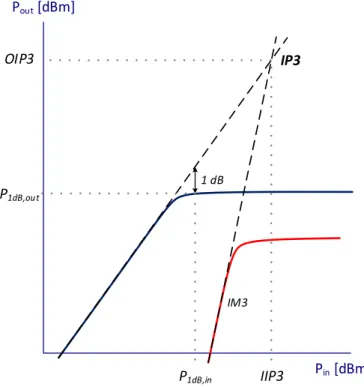
Linearity and Intermodulation Products

There is a need for an indication of the 3rd order products levels that a mixer is most likely to produce under multi-tone excitation. That spurious products in a mixer are harmonics that, when generated, can be difficult to filter without eradicating the wanted IF signal. This is problematic.

With the intersection of the extrapolated IF response with the third-order intermodulation IF product, it becomes possible to achieve this abstract point shown in Figure 2.11.

Summarising, the higher intercept point will allow to handle more input power without causing undesired products, which would interfere with the desired IF output product, and, mainly, it will allow mixer to have a greater dynamic range [17].

Pin [dBm]

P1dB,in IIP3

1 dB P1dB,out

OIP3

Pout [dBm]

IM3

IP3

Figure 2-11 – 3rd _{Order Intercept Point (IIP3).}

These calculations gives an indication of the capability of the mixer, to handle the signal. That justifies why it is so important, in terms of performance measurements of a mixer, to calculate this parameter.

2.3.2

Different Types of Mixers

Passive Mixers

18

(IF). It also explains that LO signal at high level implies an open switch, consequently, the RF input signal is transferred, and at low level the switch is off and the input signal is not transferred.

The passive mixer, which implements the mentioned process, can be designed by using CMOS transistor, shown in Figure 2.12. The gate of the transistor is driven by the LO signal, the RF signal is applied at its source and the IF signal is taken at its drain [2].

V

R

V

V

G

Figure 2-12 – Passive Mixer Using Active Device [2].

The transistor presented operates as a switch, because the LO signal induces voltage variation on the gate, which changes the operation region of the transistor. More specifically, and with the help of the equation 2.13, whenever the voltage of LO exceeds the voltage of the RF by at least a threshold voltage (_𝑉𝑇𝐻) the transistor will conduct.

{ 𝑉_{⁡⁡⁡𝑉}𝐿𝑂− 𝑉𝑅𝐹 ≥ 𝑉𝑇𝐻,⁡⁡⁡⁡⁡⁡⁡⁡⁡⁡⁡𝑆𝑤𝑖𝑡𝑐ℎ⁡𝑜𝑛

𝐿𝑂− 𝑉𝑅𝐹 < 𝑉𝑇𝐻,⁡⁡⁡⁡⁡⁡⁡⁡⁡⁡⁡𝑆𝑤𝑖𝑡𝑐ℎ⁡𝑜𝑓𝑓 (2.13)

Basically, the transistor will swing between the cut-off region (transistor off) and triode region (transistor on).

Active Mixers

In this type of mixer, the mixing operation is achieved with the same commutation behaviour mentioned previously, yet a differential pair is used instead of using a single active device. These transistors operate in the saturation region (when active) and they acquire not only a current gain, but also a high output impedance, which allows to achieve gain. Not to mention that a differential output is retrieved and, consequently, the amplitude of the IF output is doubled [1, 17].

The alternatives, that are discussed here, are named as: Single-Balanced and Double-Balanced Mixers. The first architecture is represented in Figure 2.13.

V

M1 M2

R

R

V

M3

V

V

-V

Figure 2-13 – Single Balanced Mixer [1].

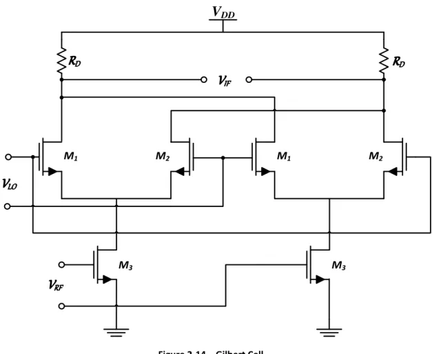
This mixer has a differential pair of inputs driven by LO signal and also has a RF unbalanced input signal, which is converted into a current and this current is drawn alternately by the two sides of the differential pair. This mixer is a simple active mixer that allows to achieve a moderate gain and noise figure and high input impedance. As disadvantages, it has low 1dB compression point, low IIP3 and low isolation on port-to-port.

20

M1 M2

R

M3

V

M1 M2

R

V

M3

V

V

Figure 2-14 – Gilbert Cell.

3

Oscillators

At this particular chapter, it is plausible to begin the explanation related to one of the most important blocks in a receiver, since the quality of a down-conversion depends on the quality of his work. In this sense, it is the oscillator and it can be said that it converts a given DC level in pure sine or square-wave signal.

The performance and some other important parameters of the oscillator, in terms of measures, will be detailed and characterized in the present chapter [1, 18, 19].

3.1

Barkhausen Criterion

It is well known that the basic function of an oscillator is to convert a DC signal into a periodic signal. A sinusoidal oscillator generates a sinusoid with frequency _𝜔0 and amplitude _𝑉0, that is:

𝑣𝑂𝑈𝑇(𝑡) = 𝑉0cos(𝜔0𝑡 + 𝜃0) (3.1)

Regarding digital applications, it is fair to mention that oscillators generate a clock signal, which is a square-waveform with period _𝑇0. Sinusoidal oscillators can be analyzed as feedback systems, shown in the next Figure, with the transfer function given by (3.2):

𝑣𝑜𝑢𝑡(𝑗𝜔)

𝑣𝑖𝑛(𝑗𝜔) =

𝐴(𝑗𝜔)

1 − 𝐴(𝑗𝜔)𝛽(𝑗𝜔) (3.2)

22

β

A

∑

V

V

+

Figure 3-1 – Simple feedback system [1].

The necessary conditions regarding the loop gain for steady-state oscillation with frequency _𝜔0 are known as the Barkhausen conditions.

It is very important to highlight the aforementioned conditions, since they play a vital role in the field of electronics. The loop gain (as show in Figure 3.1) must be unity (gain condition), and the open-loop phase shift must be _2𝑘𝜋, where _𝑘 is an integer including zero as it can be seen at (3.3) (phase condition).

|𝐴(𝑗𝜔0)𝛽(𝑗𝜔0)| = 1

(3.3)

𝑎𝑟𝑔[𝐴(𝑗𝜔0)𝛽(𝑗𝜔0)] = 2𝑘𝜋

The Barkhausen criterion gives the necessary conditions for stable oscillations, but not for start-up. For the oscillation to start, triggered by noise, when the system is switched on, it is mandatory that the loop gain must be larger than one, |𝐴(𝑗𝜔₀)𝛽(𝑗𝜔₀)| > 1.

3.2

Phase-Noise

Phase noise is an important measure of performance of an oscillator. Ideally an oscillator should generate a perfect sine-wave which corresponds in the frequency domain to two Dirac signals. According to what we said above, the output signal presents a corruption of its spectrum (3.1).

Figure 3-2 – Ideal Carrier and Carrier with Phase-Noise (adopted from [17]).

ℒ(∆𝜔)=𝑃(∆𝜔)_𝑃(𝜔

0) (3.4)

The arising of the components previously indicated as noisy sidebands, can compromise the receiver performance. If the receiver mixer performs a down-conversion using an oscillator signal with a considerable amount of phase noise, it could happen that nearby frequencies from the signal of interest can be also down-converted (Figure 3.3). Clearly, this situation will result in overlapped signals (aliasing) which is not wanted [17]. This is the main reason why phase-noise measurement can be useful to quantify the receiver immunity level against nearby channels.

Figure 3-3 – Phase-Noise Effect in Down-Conversion (adopted from [17]).

24

devices, the second region is the white noise within the oscillator and the last one is the white noise introduced by neighbor devices.

Figure 3-4 – Phase-Noise Single Side Band (adopted from [17]).

3.3

Quality Factor

The quality factor is another way of characterizing the carrier spectrum, given the fact that it is related to the oscillator phase-noise (see Figure 3.5). Considering a second order system, there are three plausible designations or definitions for the quality factor.

ω ω ω

𝑦 (_𝑥∗ 𝑥)

ωo ωo ωo

Higher Q

Higher B

Q=1 Q=10 Q=30

1. The first definition is related to a second order resonant circuit with bandwidth measured at -3db of the output signal and a carrier frequency _𝜔0:

𝑄 =𝜔_𝐵0 (3.5)

This is applied to filters and oscillators characterized as second order resonator circuits [1].

2. The second designation is expressed as the measure of the rate of how the energy is lost, regarding to the oscillator stored energy (usually the loss of energy is related to resistive devices and the stored energy with the reactive devices). This is typically applied to a generic RLC circuit and the equation 3.6 expresses the ratio previously discussed:

𝑄 = 2𝜋𝑀𝑎𝑥𝑖𝑚𝑢𝑚⁡𝑒𝑛𝑒𝑟𝑔𝑦⁡𝑠𝑡𝑜𝑟𝑒𝑑⁡𝑖𝑛⁡𝑎⁡𝑝𝑒𝑟𝑖𝑜𝑑_{𝐸𝑛𝑒𝑟𝑔𝑦⁡𝑑𝑖𝑠𝑠𝑖𝑝𝑎𝑡𝑒𝑑⁡𝑖𝑛⁡𝑎⁡𝑝𝑒𝑟𝑖𝑜𝑑} (3.6)

3. The third definition takes into consideration, not only the amplitude (A) but also the phase (_𝜃) variations of the open-loop transfer function, _{𝐻(𝑗𝜔)}, of the oscillator (which is considered as a feedback system). This definition is often considered to calculate the quality factor of a two-integrator oscillator.

𝑄 =𝜔₂0√⁡⁡(𝑑𝐴_𝑑𝜔)2+ (_𝑑𝜔𝑑𝜃)

2

(3.7)

The quality factor has an inherent relation with the phase noise, that is, the higher the quality factor more the slopes 1/f3 _{and 1/f}2 _{will come close to the carrier frequency which} reflects on the decrease of the phase noise [17].

26

3.4

Examples of Oscillators

3.4.1

LC Oscillator

In Figure 3.6 it is possible to notice the first example presented. To assure the phase shift for oscillation, the LC Oscillator uses pure reactance feedback. Like the CMOS mixers, this circuit acts as a commutator, and is constituted by a differential pair that alternate the current conduction path through the feedback network. The alternate signal is created then.

V

M

M

L

L

V

C

V

I

C

Figure 3-6 – LC Oscillator [1].

L

R

C

-1/g

m

Figure 3-7 – LC Oscillator Linear Model.

The main drawback of this kind of oscillator lies on its low frequency tuning capability, since the feedback network parameters are fixed (equation 3.10). On the other hand, a quasi-linear behaviour, low phase-noise and usually a high quality factor represent some of the advantages of the LC oscillators.

𝜔0= 1

√𝐿𝐶 (3.10)

In terms of CMOS technology area consumption, LC oscillators integration have not the most desirable area consumption. Completing, modern receivers require quadrature outputs, which this oscillator alone is not able to provide. The solution lies in coupling an additional oscillator, which will increase even more the area used as well as it will degrade the frequency response due to the additional parasitic capacitances [17].

3.4.2

Relaxation Oscillators

In the last years, most of the attention was held to another type of oscillators. Known as RC oscillators (the feedback network is now formed by a capacitor and a resistor) with very similar structure and behaviour to the ones studied in the LC oscillator. Equation 3.8 shows the integrator effect of the capacitor, transforming the DC current into voltage. The resistor is used for biasing purposes [17].

𝑣(𝑡) =1 𝐶∫ 𝑖(𝜏)

𝑡

𝑡0

𝑑𝜏 + 𝑣(𝑡0) (3.8)

28

is responsible for the loss compensation and commutation behaviour. A common RC oscillator (Relaxation Oscillator) can be observed in Figure 3.8 and the resonant frequency is shown in equation 3.9, where it was given by [1] that this oscillator integration constant is _𝐼/𝐶, and the amplitude is _4𝐼𝑅.

V

M1 M2

R

R

V

C

V

I

I

Figure 3-8 – Relaxation Oscillator [1].

3.4.3

Coupled Ring Oscillators

The most basic CMOS ring oscillator employs an odd number of static single-ended inverters as delay cells ( as shown in Figure 3.9).

0_˚ 240_˚ 120_˚

Figure 3-9 – 3-stage single-ended ring oscillator.

The transition travelling around the ring has to pass through each inverter twice to arrive at the initial state. Therefore, the oscillation frequency is given by Equation (3.10).

Unfortunately, quadrature outputs require a ring with an even number of stages [34]. Although coupled ring oscillators are not very conventional, they can provide high speed operations as well as multiphase quadrature outputs. This specially designed, single ended, inverter based coupled ring oscillators are also attractive for the capability of generating quadrature outputs in different variations. Before presenting different varieties of coupled oscillators, it is possible to say that this kind of oscillators may be useful in noisy environments. When compared with conventional ring oscillators, coupled ring oscillators have better phase noise and jitter performance, for a given power dissipation and oscillation frequency [20].

30˚ 270˚

0˚ 240˚ 120˚

150˚

Figure 3-10 –Two sets of 3-stage ring oscillators coupled together [20].

In Figure 3.9 is shown two conventional, single ended, three stage ring oscillators [21]. In order to produce multi-phase outputs and high speed oscillation, they are coupled together. This simple linear model of the ring oscillator is used to predict the oscillation frequency of the coupled oscillator. Creating three sets of outputs with 30° phase difference between the neighbour vertical nodes can make this structure to oscillate. To be able to prove that this coupled oscillator is 1.57 times faster than conventional three-stage ring oscillator frequency, [20] were done analytical studies to find a valid function of the transfer matrix of the system. Moreover it is possible to say that compared to conventional ring oscillator, this coupled ring oscillator has double the area occupied by the conventional one and dissipates also the double of the energy supplied.

Another way to produce the quadrature outputs was reported by [10], using a three stage coupled ring oscillator. But this time, were added two delay cells to couple the conventional ring oscillators in Figure 3.9. This ring topology can produce two sets of quadrature outputs with 90°

𝑓𝑜𝑠𝑐=_{2 ∗ 𝜏}1

𝐶ℎ𝑎𝑖𝑛 =

1

30

phase shift as shown in Figure 3.10, and is considered as a Quadrature four-stage ring oscillator [34]. When comparing to conventional ring oscillators performance, it is possible to say that these coupled oscillators have better phase noise, and that the oscillation frequency turns to be just the same as the conventional, single ended, inverter based version of the ring oscillator. In the next chapter a particular coupled ring oscillator will be detailed, the 8-Phase Ring Oscillator, where more useful considerations will be made.

0

˚

180

˚

270

˚

90

˚

Figure 3-11 – Quadrature four-stage ring oscillator [34].

In contrast to a ring oscillator with an odd number of inverters, now two transitions are travelling through the ring. Therefore, the oscillation frequency in now given by Equation 3.11.

As there is a rising and falling transition ate any time, the single-ended quadrature ring oscillator draws a nearly constant supply current and minimises switching noise on supply lines. To finally settle this chapter, [22] describes a way to use coupled ring oscillators, to generate accurate delays (with a resolution equal to an inverting buffer delay, divided by the number of rings). Figure 3.11 shows what it a two-dimensional array oscillator. The concept is to force numerous rings to oscillate at the same frequency. This way, each frequency can be evenly shifted in phase by an exact fraction of a buffer delay. Nevertheless, the oscillation frequency is controlled mainly by the number of buffers per ring regardless to the number of rings in the array. Additional output phases can be introduced, and the delay resolution will

𝑓𝑜𝑠𝑐 =_𝜏 1

𝐶ℎ𝑎𝑖𝑛 =

1

improve just by adding rings to the array. This kind of array oscillator can be realized using both single ended or differential inverting buffer.

Number of Columns

N

u

m

b

e

r

of

R

o

w

s

4

8 Phases Oscillator

4.1

Introduction

In order to describe and validate the 8 Phases Oscillator, there is a need to begin with a background introduction and the reason that led this work to be done. In [11] it was started to be developed a discrete-time (DT), harmonic rejection (HR) mixer with the objective of relaxing the RF filter requirements and reducing the noise folding, as seen in [23]. Contemporary CMOS technologies have allowed effective discrete-time, switched-capacitor (SC), applications of RF receiver front-ends. To obtain decent Image rejection, accurate I and Q quadrature signals are essential [2, 24] so, as already studied in Chapter 2, it is possible to consider low-IF front-ends, to overcome some of the restrictions of the zero-IF approach (mainly flicker noise and DC offset). When compared to active mixers, the passive Mixer/IIR filter used in [23], have the benefits of low power consumption when dealing with RF signals, and considerable smaller

flicker noise (as there isn’t any DC current) [2, 24]. But the central drawbacks of passive mixers is the lack of conversion gain, which disturbs the global gain and entire noise budgets for the whole receiver. To beat this limitation, [11] suggest to apply the MOS Parametric Amplifier (PA) technique to the Mixer/IIR filter proposed in [23].

Analog and DT SC mixing receiver designs from [23] can combine quadrature mixing for I/Q demodulation and wideband HR. Although, its circuit suffers from signal attenuation and forces higher gain and linearity requirements on the LNA. A charge-transfer low-pass (LP) SC filter [2] can be used, which includes a passive SC amplifier cascaded with a recursive SC filter (IIR), in order to amplify the signal amplitude. The circuit projected in [11] alone consumes 4.2 mW and occupies 0.11 mm2, without having the mixing stage into account. It also uses PA to increase the gain with reduced power and much lower area.

34

4.2

Downconverter Architecture

The SC downconverter offered by [11] associates quadrature (I/Q) mixing and wideband HR in the VHF-III band (174 to 248 MHz). In Figure 4.1 is possible to see the block diagram of the IC from where the 8 Phases Oscillator in study, was adopted. An input-driver containing a low-gain RF amplifier and two enhanced voltage-followers (EVFs) drives the fully-passive SC core

circuit. Once the objective of this IC is only to measure the SC core circuit performance, it’s

possible to say that it have about 0 dB conversion gain and provides 50 Ω input matching. The

SC downconverter core consists of three stages:

- An oversampler with fs = 8 fc (fs is the sampling frequency and fc the carrier frequency);

- Two I/Q DT mixers for downconversion; - Two LP IIR filters.

At the output, there are four simple source-followers (SFs). And, finally, the main subject of this thesis, an on-chip local oscillator (LO) that provides the required 1/8 duty-cycled clock phases to drive the SC circuit presented in [11].

Figure 4.2 shows the oversampler/mixer/IIR circuit (SC core) which encloses eight time-interleaved sampling units (SU) controlled by an 8-phase non-overlapping clock with 12.5 % duty-cycle phases ф0 - ф7 (there is a total of 16 SUs in the differential implementation) produced

by the LO.

Figure 4-2 – SC core of the downconverter (adopted from [11]).

4.3

Circuit Blocks: Sampling Cell and Local Oscillator

4.3.1

Sampling/IIR filter cell

Figure 4.3a shows a SU in detail, which embraces four NMOS I/O bootstrapped switches, driven by two clock-bootstrapping circuits (CBT), two NMOS switches, and two sampling capacitors. During fs, input switches turn ON, and the input signal is sampled into C1 and C2,

while фm perform the mixing function and фr the reset one. The wanted IIR filtering is realised

through the charge sharing between the sampling (C1, C2) and buffer capacitors (Cb). In [11], C1 and C2 were realised based on a double complementary NMOS (M1, M4) and PMOS (M2, M3) varactor structure, contrarily from [23], as shown in Fig. 4.3b. In order to reduce sensitivity to overlap parasitics, and, thus, getting the most out of the parametric gain, two internal terminals from the SU are left floating.

36

The basic SC circuit works as follows: while the gates of the varactors are connected to the input (the drain terminals of M1, M4 and of M2, M3 are connected to VDD and VSS,

respectively), it is called sampling phase (фs) and the varactors are operating in inversion mode. During the amplification phase, the four varactors have their gates connected to the output (the drain terminals of the PMOS and NMOS transistors are switched to VSS, and to VDD, respectively, forcing the varactors to operate in the depletion mode). Since the varactors capacitances drop when they move from inversion into depletion, it turns possible the parametric amplification (PA) [25].

4.3.2

The Local Oscillator

A LO based on an eight-phase ring oscillator is accessible on-chip (Fig. 4.4). It uses 16 current starved single-ended inverters. Eight in the main loop together with eight connected as latches, in between opposite nodes of the main loop.

A B C D E F G B

C Φ2

A B Φ5

C

D Φ7

D E Φ4

E F Φ1 H A Φ0 G H Φ3 F G Φ6

H Duty Cycle _12.5%

Φ

Φ

Φ

Φ

Φ

Φ

Φ

Φ

1/f

1/f

Figure 4-4 – (a) Local oscillator; (b) 8-phase 12.5 %-duty-cycle wave forms.

been used. This LO has a phase error below 1º in all eight phases [11], essentially avoiding phase overlapping, which is vital for proper mixing process.

Considering _{𝑘𝑁= 3 ∗ 𝑘𝑃}, _{𝑉𝑑𝑠𝑎𝑡𝑁 = 𝑉𝑑𝑠𝑎𝑡𝑃} and _{𝐿𝑁 = 𝐿𝑃} Then _{𝐼𝑑𝑁 = 𝐼𝑑𝑃 ⟺}1

2∗ 𝑘𝑁∗ 𝑊𝑁

𝐿𝑁 ∗ 𝑉𝑑𝑠𝑎𝑡𝑁

2₌1

2∗ 𝑘𝑃∗ 𝑊𝑃

𝐿𝑃 ∗ 𝑉𝑑𝑠𝑎𝑡𝑃

2_⟺

⟺ 𝑘𝑁∗ 𝑊𝑁= 𝑘𝑃∗ 𝑊𝑃⟺_𝑊𝑊𝑃

𝑁= 3

(4.1)

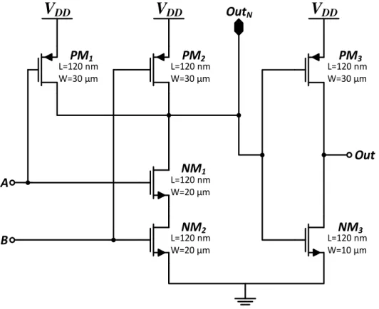
NAND

The conventional CMOS gate NAND has the configuration of the Figure 4.5. It is constituted by two blocks, a PMOS block (pull-up) and a NMOS block (pull-down). The output

should be ‘0’ only if the inputs control the NMOS block to connect the ground to the output. The same happens to the relation with PMOS, Vdd and the ‘high’ value of the output [28].

A B PM1 NM2 PM2 NM1 Y

V

Figure 4-5 – NAND gate schematic.

38

Table 4.1 – Truth table of a NAND gate.

A B Y

0 0 1

0 1 1

1 0 1

1 1 0

What to do next is considering the transistors dimensioning (PMOS/NMOS ratio adopted was 3). And the essential to get about this, as said in [28], a NAND with N inputs has a certain relation with the inverters studied before

(𝑊 𝐿⁄ )𝑛𝑁𝐴𝑁𝐷 = 𝑁 ∗ (𝑊 𝐿⁄ )𝑛𝐼𝑁𝑉 (4.2)

as NMOS relation and

(𝑊 𝐿⁄ )𝑝𝑁𝐴𝑁𝐷 = (𝑊 𝐿⁄ )𝑝𝐼𝑁𝑉 (4.3)

as PMOS relation.

In Figure 4.6 is possible to see how does the AND block create the 12,5% duty cycle with strategic 50% duty cycle inputs.

A

B

Φ

B Φ5

Figure 4-6 – Transformation of 12,5% to 50% duty cycle wave.

4.4

8 Phases Oscillator Architecture

Regarding to the eight phases oscillator, before the presentation of the final architecture,

it is important to mention the starting point, that is, the “basic circuit” that allowed the

development of the present oscillator.

Indeed, Figure 4.6 shows the “initial” circuit that was the motto for the project later

In this Chapter the most relevant premises associated to the configuration of the eight phases oscillator, were detailed with the maximum possible depth.

Thus, it would be redundant to emphasize considerations previously discussed. At this level, especially in this particular chapter, it is crucial to highlight the objectives related to the configuration presents, which led the basic circuit to a more robust architecture. From a practical point of view, the designation of the number of each phase, differs from the number regarding the phases that constitute Figure 4.4.

In other words, while in Figure 4.4, phases vary from _𝜙0 to _𝜙7, in terms of development were considered phases from _𝑝ℎ1 to _𝑝ℎ8 and the ones from A to H became out1 to out8. The phase inverted outputs are represented with the following approach: by adding the letter ‘n’ to

the respective name of each output (Figure 4.6).

The main purpose of the first part of the present dissertation, consists of developing an eight-phase oscillator capable to operate for a 400 MHz to 1 GHz range.

Evidently, the realization of this goal required changes and optimizations of the circuit initially aforementioned.

To make absolutely clear all the most relevant decisions taken, it is fundamental to detail not just the set of options chosen, since the first stage of the present work, but also highlight the reason that led to the evolution of the circuit.

Thus, the original oscillator is related to the domain of another project [11]. Regardless this fact, let it be known that in that particular project was given only an example of realization for 400 MHz.

Core

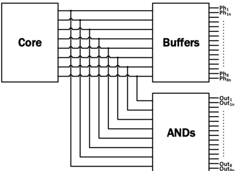
Buffers

ANDs

40

It was considered relevant to carry out the study of this particular oscillator, for a couple

of reasons: not only because on a past subject of the course (“Oscillators and PLLs”) was developed an eight phase clock oscillator that functioned approximately in 630 MHz range, but also because it was a firm conviction that it was possible to evolve the circuit in order to operate for a 1 GHz range.

4.5

8 Phases Oscillator Sizing

After presenting the global architecture, it is time to detail its constitution, that is, individualize every single relevant element, present in the circuit.

Out of respect to the work previously developed by colleagues, design process of past project was considered.

4.5.1

Inverters

Taking into consideration this fact, Figure 4.7 is shown, related to Outside and Inside Ring Inverters.

In

Out

PM

NM

L=120 nm W=30 µm

L=120 nm W=10 µm

I

I