A Work Project, presented as part of the requirements for the Award of a Master’s Degree in Finance from the NOVA – School of Business and Economics.
THE U.S. AND EUROPEAN M&A CYCLES: A MARKOV
SWITCHING AND STATE SPACE APPROACH
JOSÉ MARIA PINTO DE FARIA DA CUNHA CORDOVIL # 385
A Project carried out on the Corporate Finance course, under the supervision of Professor Paulo M. M. Rodrigues
THE U.S. AND EUROPEAN M&A CYCLES: A MARKOV SWITCHING AND STATE SPACE APPROACH 1
Abstract
Mergers and Acquisitions’ cycles have been, over the past decades, an extremely interesting field of research, raising numerous questions concerning its length, triggers or even its relationship with the economic cycle. In this Work Project I intent to contribute with new evidence, mainly for European merger waves, but also to support previous studies in what regards to merger waves. I have chosen nonlinear models, such as the Markov Switching and the State Space models, to characterize the merger data, due to the advantage of identifying structural changes. I have concluded that there is evidence of merger waves, both in the U.S. and in Europe, and the possible surge of a new merger wave in Europe.
Keywords: Mergers and Acquisitions, Nonlinearity, Structural Changes, Markov
Switching, State Space.
1 I am very grateful to Professor Paulo Rodrigues, for all his insightful suggestions and support in the development of this Work Project. I would also like to thank to Professor Raúl Guerreiro for his assistance on the construction of the State Space model.
1 - Introduction
The analysis of merger waves is an old, but still fashionable and debated subject which has gathered the interest of many economists over the past century, see, e.g. Nelson (1959) and Golbe and White (1987). The number and value of Mergers and Acquisitions (M&A) has steadily grown over the last decades and its impact on the economy is seen not only as relevant at a macro level, e.g. business cycles (for instance, Becketti, 1986, examined the relationship between business cycles and merger activity, and concluded that M&A activity is strongly procyclical and is, for instance, highly influenced by changes on interest rates; but also at a micro level, e.g. industry consolidation, Chen, 2006, studied the effects of mergers in terms of welfare). This empirical study will focus on a macro perspective rather than on a micro, since the objective is to understand the M&A cycles over the past thirty years, and not to assess how M&A waves impact society in terms of value creation / destruction2. Therefore, one of the main challenges will be the development of appropriate models which capture the stochastic behavior of M&A and forecast its activity.
The study of this subject has always been significantly conditioned by the available statistical understanding. Before the seminal work of Hamilton (1989), who argued that U.S. real GNP could be modeled as a Markov-Switching (MS) process, where the transition between states is determined by a first-order Markov process, the most frequently used techniques to model this type of series were linear models, such as Autoregressive (AR), Moving Average (MA) or a mix of both, ARMA, which for instance, Nelson and Plosser (1982) applied to U.S. real output. However, linear techniques are not efficient and flexible enough to capture the nonlinear movements,
2 One of the main fields of research in M&A is to assess evidence of returns on this type of activity. Robert Bruner, for instance, is well known for his extensive research in this area.
such as, asymmetries; amplitude dependence and volatility clustering, which in series like GDP or M&A are fundamental, e.g. deregulation, innovation in financial markets, corporate trends, changes in consumer demand and supply or technological changes, so as to completely understand its pattern. Nevertheless, there are researchers who support that linear models can described M&A waves quite well. For instance, Barkoulas et al. (2001) claimed that the U.S. M&A activity is a strongly correlated process, which could be modeled using a fractionally integrated model, since the series presented long-memory and persistence dynamics, and consequently there would be no need to use nonlinear models.
Hence, there is still no unanimous view on which functional form, linear or nonlinear, is the most adequate to model this type of time-series. Nonetheless, it was possible to attain similar empirical evidence through different class of models, supporting the existence of a cyclical behavior in M&A activity.
MS models are one class of models frequently used to study nonlinear time-series. After the breakthrough of Hamilton (1989), many researchers started to develop further applications. For instance, Town (1992) constructed a two-state MS model for M&A activity, both for the U.S. and the U.K, and succeeded in rejecting the absence of different regimes. Later, Gartner and Halbheer (2004), instead of estimating the unknown parameters through Maximum Likelihood Estimation (MLE), applied Bayesian inference – Gibbs-Sampling, treating both parameters and the unobservable variable as random, though they have managed to produce similar results to studies using classical approaches. A commonly used simplifying assumption, frequently used in MS models, is that the transitions probabilities are constant over time. Resende (2005), based on theoretical improvements made by Diebold et al. (1994), in which a
MS model with time-varying transition probabilities (TVTP) was proposed, developed a two-state, MS model with TVTP for the U.K. M&A activity, and found evidence that one should reject the constant transition probabilities in detriment of the TVTP model, however, since in this empirical study a new analysis for the European M&A activity will be undertaken, for simplification, the TVTP model is not going to be used.
An alternative technique that also allows for regime shifts are Threshold Models (TM), see, e.g. Tong (1983) and Potter (1995). Although TM can capture switches in regimes reasonably well, there is a crucial difference, when compared to MS models, in the former, regimes are defined through a deterministic scheme, that is, one has to determine in the time-series where the structural change occurs, while in the latter regimes are treated as an unobserved variable defined by the exogenous state of a Markov chain, and thus are determined by the model and not by the researcher. Hence, albeit there is a vast literature regarding business cycles analysis, see, e.g. Beaudry and Koop (1993), there are no significant developments within this type of models concerning modeling M&A activity, mainly due to the fact there is no consensus on the M&A cycle periods, and therefore it is difficult to determine the M&A thresholds in order to construct TM models with this type of data.
Another prominent method to characterize economic and financial time-series is the State Space (SS) approach, which was first introduced by Kalman (1960). This method enables time-series to be decomposed into several components, one of them being the cyclical component. Though the application of this technique to model M&A activity has not yet been widely used, it has been successfully employed in the study of business cycles, see, e.g. Harvey (1989); Kim and Nelson (1999) and Guerreiro (2010). Thus, it appears not only worth to model M&A activity through the SS approach, but also to
compare its results to those of the MS model and to use the SS results as a validation instrument. Therefore, the models that are going to be constructed under this research will be both the MS and the SS models.
Thesis’ objective
This empirical research, as previously said, will focus on the dynamics of the merger waves both in the U.S. and Western Europe (W.E.). Whereas on the former, a considerably literature developed over the last thirty years, on the latter there is very little research. Therefore, one of the innovative features of this investigation will be the analysis of the W.E. merger data as a proxy for the European Union (E.U.), in order to assess if, for instance, there was actually a shift in the European merger activity with the introduction of the Euro, if the merger cycles in Europe are different, in terms of length and timing, from the ones in the U.S., or if the W.E. M&A activity is correlated with the U.S. Furthermore, the hypothesis constructed along this paper can draw some conclusions on the European M&A trends, and how its behavior is correlated with economic activity, which could be extremely useful to anticipate or even predict the merger cycles within the European region.
Ultimately I attempt to contribute to the current understanding of M&A cycles, more specifically to the comprehension of the European M&A taking into account the recent developments to create a common financial and political zone, which I believe to be fundamental to have a more stable merger cycle, like the one in the U.S..
Hence, the chief objectives of this empirical paper are: (i) assess the M&A cycles and its features, both in the U.S. and in W.E., where the latter is of particular interest; (ii) analyze the comovement between U.S. and W.E. M&A series, so as to evaluate
possible leads and lags in what concerns the timings of both series, and (iii) explore the relationship between M&A and economic activity.
The paper is organized as follows. Section 2 presents the data employed, Section 3 briefly describes both methods used, and how inference and estimation is carried out, Section 4 presents the estimation results and the empirical findings, and finally Section 5 offers some final comments.
2 - The Data
In order to choose the most appropriate proxy for M&A activity, two possible variables may be considered: (i) the number of transactions and, (ii) the aggregate dollar value. The former is used by Linn and Zhu (1997) and Gartner and Halbheer (2004), whereas the latter is applied, for instance, by Golbe and White (1988). In this paper the number of deals will be chosen in detriment of the aggregate dollar value. The main argument to support this decision is that the number of transactions best reflects the breadthof M&A activity, whereas the aggregate dollar value is highly dependent on exceptional deals, which can deceive the understanding of M&A waves and consequently its modeling.
In what concerns the data itself, for the U.S. activity the transactions in which the target was an U.S. company, from Q1 1980 until Q2 2012, were considered and for Western Europe the same reasoning was employed, though for a shorter period, from Q1 1982 until Q2 2012, due to lack of data. Quarterly data was selected in order to reduce the noise of less aggregated data, e.g. monthly data, which at the same time, have a more detail view on the evolution of the merger activity over the past thirty years. The data was collected from the financial platform ThompsonONE.com Deals3.
3 Excluding Debt Tender Offers; Equity Carveouts; Exchange Offers; Loan Modifications; and Open Market Repurchases. All pending and complete deals are comprised in both series.
In the figures below, two graphs regarding the number of transactions are presented, one for the U.S., and the other for Western Europe. At a first glance M&A activity appears to have a time trend and one could argue that a linear model would be suitable to characterize this set of data. However, in this type of financial data, there are structural changes which can be detected in the figures below. For instance around the year 2000 there is an abrupt swing in the number of deals in the U.S., and in order to take these structural shifts into account non-linear models may be suitable.
As described in the previous chapter, the 1980s’ merger wave both in the U.S. and in W.E. can be perceived and also the merger wave of the 1990s, which had its peak around the year 2000. Finally, as the literature suggests, the merger wave of 2000s is also evident. These data will be the raw material of the models that I am going to developed in the following chapter, in order to support the previous merger waves’ hypothesis, developed over the past years, and hopefully, to construct new hypothesis based on the output of the models and its subsequent analysis.
3 – The Methodology
In order to test for cyclical behavior in merger activity, in this section, two different approaches will be presented. The first is the Markov-Switching [MS] model which will be based on the work of Hamilton (1989) and Town (1992), while the second is the State Space [SS] approach which will be centered on the work of Kalman (1960). There will be more details on the MS model, as this is the head model of this paper, nonetheless the SS model will be extremely valuable since it will be used as an assessment tool and will help emphasize the MS model’s results.
When dealing with time series, more specifically financial data, one of the central challenges is to model the conditional expectation of a series, which is very likely to change over time due to, for instance, structural changes. Hence, to account for fluctuations in the conditional mean, models such as the MS and the SS are very useful as they capture those oscillations, and therefore are able to provide consistent output to develop and build reasonable statements.
Before introducing both models, the first step is to observe if M&A activity in the U.S. and in W.E. is stationary. This is an important step since the MS model that is going to be developed is based on an auto-regressive representation. From the application of the
ADF unit root test, it is concluded that the U.S. and the W.E. M&A activity are stationary4. The U.S. M&A activity follows an AR(1) process while the W.E. M&A activity follows an AR(2) process.
3.1 - Markov-Switching Model
The Markov Switching model that is going to be considered in this dissertation is a univariate auto-regressive MS model, where the changes in regimes will be governed by a two-state Markov chain. The main feature of this technique is that it accounts for abrupt variations in the conditional mean and variance of a time series, e.g. structural changes, so that it combines two or more dynamic models. In (3.1.1) a simple MS AR(1) process is presented, the one which is going to be used to model the U.S. M&A activity,
{
, (3.1.1) where the AR coefficient, |β| < 1, and is an i.i.d. random variable with zero mean and variance . As expressed in equation (3.1.1), the M&A activity, , is dependent on the value of , which can be either 1 or 2 (being 1 in the low-state, and 2 in the high-state of merger activity). At a first glance, one could argue that this model is simply constructed as two different linear equations, whereas one has a dummy variable, when . However, that would only be valid if the changes between the values of were determined by a deterministic event, that is, if until a certain time , would be governed by the first equation and after by the second equation, therefore assuming that the transition between states would be determined a priori. However, is a random variable, i.e. an imperfectly predictable force that produces the correspondent
4
changes in (Hamilton, 2005). The probabilistic model that will be employed to ascertain the shifts in is known as a time invariant first-order Markov-chain, that is, ( | ( | . (3.1.2) The condition in (3.1.2) assumes that the probability of a change in regime depends only on the past regime and thus undermines the precedent regimes. Although this assumption seems convenient and simplistic, it is a good starting point and it is considerably more consistent than assuming that the swings in regimes are deterministic events. Moreover, besides the research done by Golbe and White (1993), which suggest that the U.S. M&A activity is a high memory process, recent literature justified that the M&A shifts are indeed processes with little memory.5 Note that the transition probabilities in (3.1.2), are time invariant (FTP), as opposed to the time-varying transition probabilities (TVTP) model, which assumes that the transition probabilities change over time. Although the TVTP model is more robust, (see Kim and Nelson, 1998, and Filardo, 1998), for the sake of simplicity the FTP model was the one chosen. The transition matrix, which is presented below, determines the regimes’ transition through the transition probabilities considered in (3.1.2), i.e.,
[ ( | ( | ( | ( | ] [
] . (3.1.3) As can be inferred from (3.1.3), , where . Therefore, the only two parameters of the transition matrix are and , which define the changes in regimes, and also the persistence of each regime. For instance, if and , according to what was mentioned above, the interpretation of these probabilities, in a merger context, is that the low-state is less persistent than the high-state, and therefore if we are currently experiencing high levels of merger activity
within a specific region, the probability of remaining in the same regime is higher than that of changing regime, if . Another important remark is that if or are 1, it means that the observable state is permanent, leaving no evidence of merger cycles. Nevertheless, this is a very unlikely and extreme scenario, since in the economic and financial field there are no permanent events, one clear example are the recessions, although some are extremely severe there is always an inflexion momentum.
Hence, the parameters that one has to estimate to define the transition matrix, and consequently the transition probabilities of , are the auto-regressive coefficient , the variance of the so called Gaussian innovation , both intercepts and , and finally the two-state transition probabilities and . The estimation method that will be considered is the Maximum Likelihood Estimation (MLE) method described in the following section.
3.2 –Maximum Likelihood Estimation
There are several methods to estimate MS models, either through MLE, which is usually entitled as the Classic approach (Hamilton, 1989, 1994); the Expectation Algorithm (EM) (Hamilton, 1990); or through the Bayesian methods - Gibbs Sampling (which was first developed by Albert and Chib, 1993, and used latter in an M&A context by Gartner and Halbheer, 2004). After assessing the advantages and disadvantages of these estimation methods, in the end the MLE is not only the most straightforward technique but also the most commonly applied method used in empirical applications.
Taking into consideration the model described in (3.1.1), the corresponding log likelihood function, assuming Gaussianity, is,
∑ ( √ ( )) (
If all values of were known, we would only need to maximize (3.2.1) in order to estimate the values of the parameters, , however since one of the MS model features is that is stochastic, estimation becomes more complex. If we consider, ( | as the likelihood function of for , where , conditional on , where { }, then the complete log likelihood function is,
∑ ∑( ( | ( ) (
Since the probabilities, ( cannot be observed, Hamilton (1989) proposed an iterative algorithm, to calculate the filtered probabilities, which is constantly updated with the new information available. Considering, the available information at time t-1, inference should be made through the following sequence:
i. for we assume that ( in order to trigger the process; ii. for , we have:
( | ∑ ( ( | (
where are the transition probabilities mentioned in (3.1.3), and calculate the probability of each state given the available information at ;
iii. After having the information at time , update the probability of each state given the new information through the following formula:
( | ( | ( |
iv. If we set , and repeat steps ii. and iii. until the end of the sample, a set of filtered probabilities is provided for each state, through all the observations. Therefore, in order to estimate the MS model the log like function in (3.2.5) should be maximized, i.e.,
∑ ∑( ( | ( | )
(
Note that in the empirical application below, all computations referred throughout the last two sections were performed in Matlab6.
3.3 – State Space Model
The SS model introduced in this section is based on the findings of Kalman (1960), and more recently Guerreiro (2010)7. The main idea of the SS models is to create a structural model which represents a more complex linear system, and then decompose the observed time series into its different components: trend, cyclical and error.
The first step of the process is the definition of the structural model, which you can find below (3.3.1), which according to Wada and Perron (2006) is the most widely used.
{ (
As previously indicated, the time series { }, is decomposed into three factors. The one which raises more interest to assess M&A cycles, is the cyclical factor, , which under this structure is assumed to follow an AR(2) process with ~ i.i.d. ( .
After considering the structural model, (3.3.1), we must represent it in a state space model framework, such as,
6
The Matlab code used was developed by Marcelo Perlin (2012). 7
[ ] [
] (
which can be expressed as, , assuming that [ ]. The following step is to define the transaction equation, which defines a relationship between the actual state and the previous one, assuming that the state follows a first order Markov process. Thus, the transaction equation is characterized as8:
[ ] ⌈ ⌉ [ ] [ ] [ ] ( (
where and , being constant over . Since the SS model that represents M&A activity, (3.3.2), and its transaction equation, which governs the link between the states, (3.3.4), are defined we can proceed to the estimation process through the Kalman filter.
3.4 – Kalman Filter
This filter is somehow similar to the estimation process of the MS model, where Hamilton (1989) proposed an iterative method based on MLE to estimate the unknown parameters. However there is one crucial difference to the MS model, which is how the initialization process is triggered. In order for the Kalman filter to be effective, an initial distribution for or at least the determination of ( and for the (
must be considered, the method that is intrinsic in the estimation code is the diffusion
8 A more detailed explanation of the transaction equation can be found in Guerreiro,“Filtro de Kalman, filtro Hodrick-Prescott,
initialization9. Therefore, taking into consideration (3.3.2) and (3.3.4), the unknown parameters which maximize the likelihood function are [ ]. The method for determining the optimal values of the vector is based on a non-linear search10.
Once the vector is determined, the several components of the state space model defined in (3.3.1) can be estimated11, and consequently the cyclical component, can be extracted from the model12.
4 – Results
In this section the estimation results of the MS and the SS models, described in the previous section, are presented. A comparison with previous empirical studies is also offered. The U.S. M&A activity will be analyzed first, followed by the results for W.E.. Below you can find a table summarizing the findings of the MS model.
9 Koopman, Wang and Zivot (2004), Wada and Perron (2006) and Guerreiro (2010)
10 The method chosen by Guerreiro (2010) was the framework proposed by Clark (1997) and by Kim and Nelson (1999) 11 The remaining components of the State Space model can be found in the Appendices.
12 Although I have used the number of deals as the input for the MS model, for the SS model I have used the logarithm of the number of deals.
Table 1 - Summary of MS models’ output
U.S. Western Europe
p11 92.08% 90.81%
p12 7.92% 9.19%
p22 91.86% 84.87%
p21 8.14% 15.13%
Expected Duration of Regime #1 12.62 10.88
4.1 – U.S. M&A activity
The U.S. M&A observations are from 1980:Q1 until 2012:Q2, as expressed in Figure 1, which comprises more than 30 years of merger activity. Economists have been characterizing M&A waves for the U.S. for some years and there is some consensus on that matter, despite the lack of supporting models. Therefore, the results of the models, constructed throughout this empirical research, will be compared with the historical awareness that has been developed over the last years, in order to validate, or not, the hypotheses of merger waves.
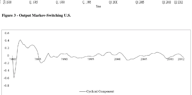
During this period, the first wave is considered to have started at the beginning of the 1980s, caused by a set of factors, such as: (i) deregulation, as the Kemp-Roth Tax Cut in 1981, known as the “Reagan Tax Cuts”, which essentially simplified the tax code, reducing the amount of deductions and the number of brackets; (ii) during the 1960s there was an attempt to conglomerate or diversify companies revenue streams, whereas this vision was discarded in the 1980s by being too complex, “It’s not that
conglomerates are difficult for analysts to understand. We worry that conglomerates are difficult for management to understand”13
, and therefore managers started to restructure and divesture, since being a conglomerate was no longer seen as an advantage; (iii) more innovative financial products e.g. issuing junk bonds to finance takeovers or more leverage, that eventually led to an increase in the level of M&A activity. As can be seen in Figure 3 (MS model) and Figure 4 (SS model), the output of both MS and SS models clearly identify the 1980s merger wave, although the merger wave is more persistent in the MS model, there is evidence of a cyclical behavior in the 1980s, which is also supported by past studies (Town, 1992 and Linn and Zhu, 1997). According to the output, particularly of the MS model, this wave ends around 1986 and
1987 matching with the U.S. economic slowdown and the 1987 “Black Monday”. Nevertheless, the empirical study of Gartner and Halbheer, 2004, did not succeed to identify the 1980s’ merger wave. One possible explanation may be the fact that they applied Gibbs sampling for inference, while the remaining studies used MLE.
The second merger wave, for this period, took place after the recession of 1990-1992, which was characterized by the jump in oil prices, due to the Gulf War, associated with a decrease in consumer confidence, a high leveraged economy and a drop in real estate prices. However the situation changed in late 1992. M&A activity started to upturn considerably, where strategic buyers were now more active, so as to pursue synergies, rather than the financial buyers during the 1980s, where very large deals
Figure 3 - Output Markov-Switching U.S.
occurred to enhance synergies, as Worldcom / MCI Communications, BP / Amoco or Daimler-Benz / Chrysler. There was a special feature of this wave, as there was a sector-focused activity in industries such as the banking, healthcare, defense and technology. Furthermore, the high level of M&A activity, during this period, matched with historically low interest rates and rising stock prices, culminating in the Internet bubble of March 2000. If we investigate Figures 3 and 4, we succeed in identifying a merger wave for this time frame, which again, reveals the solidness and reliability of both models. Moreover, in both models there is a sharp drop in the probability of a high state, which suggests an end of the 1990s merger wave. Gartner and Halbheer, 2004, were successful in identifying this wave, contrary to the one during the 1980s, hence the choice of the estimation procedure clearly influences the final output.
Lastly, concerning the 2000s merger wave some empirical studies (Alexandridis, Mavrovitis and Travlos, 2011), suggest that this wave started during 2003, peaking in 2006 and coming to an end in late 2007. This merger wave was characterized by an intense activity from Venture Capital, Private Equity and Hedge Funds firms, whereas liquidity difficulties were no longer a problem, i.e. the percentage of equity financing dropped significantly during this merger. From the models’ output this merger wave is not as clear as the previous ones, since in the MS model we have an inflexion point in 2003 [Figure 3], though not strong enough to bring the high state probabilities to levels as the ones observed in the previous waves, and thus fails to identify the last merger. Nonetheless, the SS model successfully identified this merger, demonstrating the importance of having two different models to support the argumentation.
An interesting observation, from Table 1, are the transition probabilities , which suggest that M&A states, either the low or high, in the U.S. are highly persistent,
when , and consequently when . This is better understood observing the expected duration of both merger states, which in the case of the U.S. are around 12 quarters, a considerably high figure when compared to the European proxy.
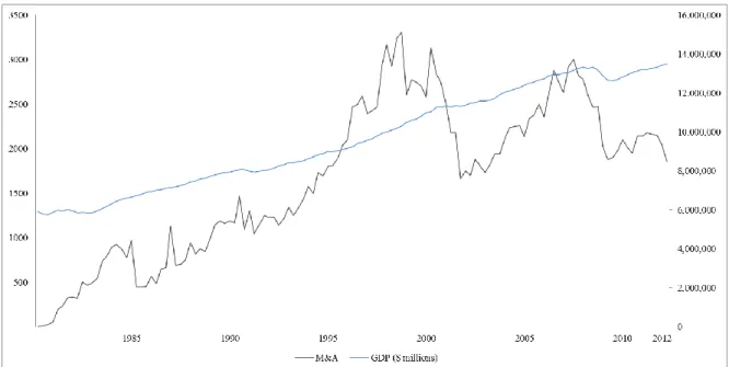
The purpose of Figure 5 is to show that U.S. M&A activity and GDP14 have a similar behavior over the past 30 years, and this could somehow shed some light on the link between merger and economic activity, which was firstly proposed by Becketti (1986). The correlation of the series suggests a very strong relationship, with a correlation coefficient of 0.83. Moreover, also with the aim to understand how the economic cycle and the level of M&A relate I have performed a lead / lag analysis, this is done through observing if the M&A series and the maximum correlation: (i) coincides with the economic activity, and therefore there is no lead / lag; (ii) the maximum correlation is found when the M&A is ahead of the economic cycle, the M&A series is understood to
14 Downloaded from Thomson and Reuters’ DataStream platform.
be lagged; (iii) the maximum correlation is found when the M&A is lagging the economic cycle, the M&A series is understood to be lead. In this particular case, the maximum correlation is achieved when the series are coincident, meaning that, together with the 0.83 correlation coefficient, both the U.S. economic and M&A activity have very similar and coincident patterns.
All in all, according to the last decades’ literature, it was possible, through both models, to successful identify the three big merger waves of the last three decades. This objective was substantially simplified by the fact that the merger waves were already defined by some authors (Martin, 2007; Bruner, 2005), nevertheless it was a particularly interesting analysis to confirm the past findings and also to compare the results of both models.
4.2 – Western European M&A activity
In what regards to the Western European activity, the task to analyze and understand merger cycles, is harder. As previously mentioned, there are no studies concerning the modeling of the Western European M&A activity, and there is also very little literature concerning European merger waves.
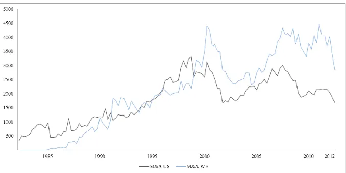
When looking at Figure 2, and in line with the U.S. graph for the M&A activity [Figure 1], there is a perceptible upward trend along the series and a cyclical behavior, which are characteristics of M&A series. However, in the output of the MS models, Table 1, the first thing that leaps out, when compared with the U.S. output, is that the transition probabilities and are higher, suggesting that W.E. merger waves are more volatile or less persistent than U.S. waves. Between 1982 and 2012 we can observe more merger cycles than for the U.S. series, particularly after the year 2000. The fact that the W.E. sample comprises different economies, with different growth
policies highly influences European M&A activity, especially the cross border deals. These are also translated into the expected duration of the regimes, whereas in the U.S.
we observe longer cycles, either in the Low (1) or High State (2), in W.E. we observe shorter cycles in both regimes, see Table 1.
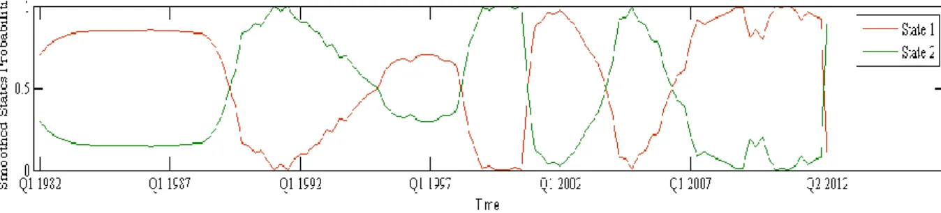
Additionally, the first two merger waves, observed from the MS model [Figure 6], the 1980s and the 1990s, appeared delayed by some periods when compared to the U.S., see Figure 8, suggesting that these merger waves started to be verified in the U.S. and only after in the W.E., which is a particularly interesting fact taking into account that the U.S. during those 20 years were by far the world’s largest economy, and thus determining the corporate trends, which could be translated into new forms of M&A waves. Also, the development and the creation of new financial products during the past
Figure 7 - Output State Space W.E. Figure 6 - Output Markov-Switching W.E.
decades occurred mostly in the U.S., as the competition among financial institutions was much more intense than in Europe, thus there was a need to innovate by developing new products in order to differentiate from the competition. In order to sustain this
hypothesis, of the W.E. M&A activity lags the U.S. M&A activity, I have performed the lead /lag analysis, aforementioned above, and determined that the W.E. M&A activity lags the U.S. M&A activity by 2 quarters, and if the correlation coefficient of 0.84 between both series is taken into account, there is enough evidence that in fact the European M&A waves are delayed to the U.S..
Moreover, the most remarkable finding is the fact that the MS model suggests that we are currently observing the beginning of a new merger wave in W.E., as can be inferred from Figure 6, which is at least surprising considering the current European financial situation, however if we take a more throughout look to the European banking system, mainly Western European financial institutions, these are currently undertaking restructuring plans by, for instance, selling non-core assets in order to comply with the
European Banking Authority capital requirements. The fact that European financial institutions, and other class of companies, are desperately seeking for liquidity, offers new business opportunities for private equity firms willing to buy distressed assets,
“There are a myriad opportunities as banks have publicly said they have more than $1 trillion of assets they need to sell and we can form partnerships with them and build businesses”15
, this is clearly a consequence of regulation changes, which in this specific case may lead to an asset sale merger wave in Europe.
When comparing the output of both MS and SS models for the W.E. activity [Figure 6 and 7], there is clear evidence of a considerable swing between both regimes, and consequently the fact that in the European region M&A activity is more prone to be affected by external shocks, such as changes in regulation, international crisis, corporate trends. Albeit both models present almost the same results, there is a small, yet importance difference, the SS model does not conceive the start of a new merger wave, hence the merger hypothesis aforementioned is only supported by the MS model.
15 Head of Kohlberg Kravis Roberts expect to make big returns from buying distressed assets in Europe as regulatory changes force banks to deleverage.
5 – Conclusion
The primary objective of this paper was to study the features of M&A waves in the U.S. and W.E., validating previous studies (Town, 1992; Linn and Zhu, 1997; and Gartner and Halbheer, 2004) and to develop new hypothesis. Regarding the U.S., the results were similar to those found in literature, although with some differences, mainly explained by the estimation methods and the period of observation. Essentially, it was possible to identify three merger waves over the last 30 years. An important remark is the fact that the MS model alone could not identify the last merger wave, highlighting the importance to have two models to support the hypothesis construction.
As expected, the most interesting findings from this research were related to the European M&A activity. First, the fact that since 2000 the M&A cycles observed in this region are much more volatile, and consequently with a shorter period length, than in previous years. This could eventually be explained by the creation of the Euro, and all the political and economic regulation that were established to support this currency, which substantially affected the Eurozone. Another important observation from this empirical study is the fact that the European M&A until the year 2000, seemed to be delayed when compared to the U.S. M&A activity, due to reasons such as corporate trends and financial innovation. Last, the most striking evidence is the possible surge of a new merger wave in Europe, due to the corporate restructuring that this economic area is suffering.
All in all, this empirical study clearly supports the M&A wave hypothesis in both U.S. and W.E., revealing extremely interesting facts about the nature and dynamics of these mergers and acquisitions waves.
References
Alexandridis, G., Mavrovitis, C.F. and Travlos, N.G. 2011. “How Have M&As
Changed? Evidence from the Sixth Merger Wave”.
Barkoulas, John T. et al. 2000. “Waves and Persistence in Merger and Acquisition
Activity”.
Beckenstein, Alan. 1979. “Merger activity and merger theories: An empirical
investigation”, Antitrust Bulletin, 24: 105-28.
Becketti, Sean. 1986. “Corporate Mergers And the Business Cycle”. Economic Review. Banco Central Europeu. 2002. “Boletim Mensal - Julho”, 41-51.
Bruner, Robert. 2004. Applied Mergers & Acquisitions. Hoboken, New Jersey. Wiley
& Sons, Inc.
Mario, Carapeto, Dallocchio, Maurizio, Faelten, Anna, Lanzolla, Mariachiaria and Moeller, Scott. 2010. “Can business expectations predict M&A activity?”.
Clarke, R., and Ioannidis, C. 1996. “On the relationship between aggregate merger
activity and the stock market: some further empirical evidence”, Economics Letters, 53: 349-356.
Crafts, Nicholas. 2011. “Western Europe’s Growth Prospects: an Historical
Perspective”.
Diebold, Francis X., Lee, Joon-Haeng and Weinbach, Gretchen C. 1994. “Regime
Switching with Time-Varying Transition Probabilities”.
Diebold, Francis X., and Rudebusch, Glenn D. 1996. “Measuring Business Cycles: A
Modern Perspective”.
Frain, John. 2008. “An Introduction to MATLAB for Econometrics”.
Gartner, Dennis, and Halbheer, Daniel. 2004. “Are There Merger Waves After All?”. Golbe, Devra L., and White, Lawrence. 1987. “Mergers and Acquisitions in the U.S.
Economy: An Aggregate and Historical Overview”, University of Chicago Press, Mergers and Acquisitions, 25-48.
Golbe, Devra L., and White, Lawrence. .1993. “Catch a Wave: The Time Series
Behavior of Mergers.”, Review of Economics and Statistics, 75, 493-499.
Gordon, Roger and MacKie-Mason, Jeffrey. 1990. “Effects Of The Tax Reform Act
Of 1986 On Corporate Financial Policy And Organizational Form”.
Guerreiro, Raul Filipe C., Rodrigues, Paulo M. M., and Andraz, Jorge M. L. G.
2011. “Filtro de Kalman, filtro Hodrick-Prescott, filtro Baxter-King e o ciclo económico português”.
Gugler, Klaus, Mueller, Dennis, and Weichselbaumer, Michael. 2011. “The
determinants of merger waves: An international perspective”. International Journal of
Hamilton, James D. 1989. “A New Approach to the Economic Analysis of
Nonstationary Time Series and the Business Cycle”. Econometria, Volume 57, Issue 2, 357-384.
Hamilton, James D. 1994. Handbook of Econometrics. Volume IV, Edited by Engle,
R.F. and McFadden, D.L., 3041-3080.
Hamilton, James D. 2005. “Regime-Switching Models”.
Higson, Chris, Holly, Sean, and Platis, Stylianos. “Modelling Aggregate UK Merger
and Acquisition Activity”.
Kim, Chang-Jin, and Nelson, Charles R. 1998. “A Bayesian Approach to Testing for
Markov Switching in Univariate and Dynamic Factor Models”.
Kim, Chang-Jin, and Nelson, Charles R. 1999. “State-Space Models with Regime
Switching: Classical and Gibbs-Sampling Approaches with Applications”, MIT Press, Cambridge, Massachussets.
Kuan, Chung-Ming. 2002. “Lecture on the Markov Switching Model”.
Linn, C., and Zhu, Z. 1997. “Aggregate merger activity: New evidence on the wave
hypothesis”. Southern Economic Journal, 64: 130-46.
Martin, Stephen. 2007. “Mergers: An Overview”.
Medeiros, Otavio and Sobral, Yves. 2007. “A Markov Switching Regime Model of
the Brazilian Business Cycle”.
Nelson, Charles R. and Plosser, Charles I. 1982. “Trends and Random Walks in
Macroeconomic Time Series”, Journal of Monetary Economics, 10, 139-162.
Olshausen, Bruno. 2004. “Bayesian Probability Theory”.
Owen, Sian. 2004. “A Markov Switching Model for UK Acquisition Levels”. Potter, Simon. 1999. “Nonlinear Time Series Modeling: An Introduction”.
Resende, Marcelo. 2005. “Mergers and Acquisitions Waves in U.K.: A
Markov-Switching Approach”.
Sheppard, Kevin. 2010. “Financial Econometrics MFE MATLAB Introduction”. Stock, James H. and Watson, Mark W. 1989. “New Indexes of Coincident and
Leading Economic Indicators”, NBER Macroeconomics Annual 1989, Volume 4, 351-409.
Tong, Howell. 2010. “Threshold Models in Time Series Analysis – 30 Years On”. Town, R. J. 1992. “Merger waves and the structure of merger and acquisition time
series”. Journal of Applied Econometrics, 7: S83 - S100.
Tsay, Ruey S. 2005. Analysis of Financial Time Series. Hoboken, New Jersey. Wiley &
Sons Inc.
Tufano, Peter. 2002. “Financial Innovation”. The Handbook of the Economics of
Appendices
Annex 1 – Output of Markov Switching Model
Annex 2 – Output of State Space Model
U.S.
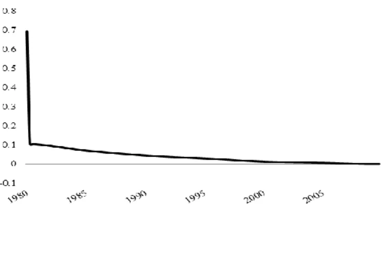
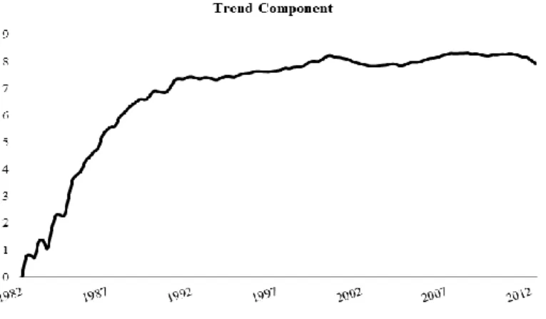
Figure 11A – Trend component of the SS model for the U.S. Figure 11B – Random component of the SS model for the U.S.
Western Europe
Figure 12A – Trend component of the SS model for the W.E. Figure 12B – Random component of the SS model for the W.E.