Dimitri Nowicki1,2*, Patrick Verga1
, Hava Siegelmann1,3*
1The Biologically Inspired Neural and Dynamic Systems (BINDS) Lab, Department of Computer Science, University of Massachusetts Amherst, Amherst, Massachusetts, United States of America,2Institute of Mathematical Machines & Systems Problems of NASU, Center for Cybernetics, Kiev, Ukraine,3Program of Neuroscience and Behavior, University of Massachusetts Amherst, Amherst, Massachusetts, United States of America
Abstract
Memory reconsolidation is a central process enabling adaptive memory and the perception of a constantly changing reality. It causes memories to be strengthened, weakened or changed following their recall. A computational model of memory reconsolidation is presented. Unlike Hopfield-type memory models, our model introduces an unbounded number of attractors that are updatable and can process real-valued, large, realistic stimuli. Our model replicates three characteristic effects of the reconsolidation process on human memory: increased association, extinction of fear memories, and the ability to track and follow gradually changing objects. In addition to this behavioral validation, a continuous time version of the reconsolidation model is introduced. This version extends average rate dynamic models of brain circuits exhibiting persistent activity to include adaptivity and an unbounded number of attractors.
Citation: Nowicki D, Verga P, Siegelmann H (2013) Modeling Reconsolidation in Kernel Associative Memory. PLoS ONE 8(8): e68189. doi:10.1371/ journal.pone.0068189
Editor:Maurice J. Chacron, McGill University, Canada
ReceivedMarch 6, 2013;AcceptedMay 27, 2013;PublishedAugust 2, 2013
Copyright:ß2013 Nowicki et al. This is an open-access article distributed under the terms of the Creative Commons Attribution License, which permits unrestricted use, distribution, and reproduction in any medium, provided the original author and source are credited.
Funding:This research was supported by Office of Naval Research (ONR) grant AWARD#N00014-09-1-0069. The funders had no role in study design, data collection and analysis, decision to publish, or preparation of the manuscript.
Competing Interests:The authors have declared that no competing interests exist.
* E-mail: nowicki@cs.umass.edu (DM); hava@cs.umass.edu (HS)
Introduction
Memory reconsolidation (ReC) is a recently proposed process explaining the update of long-term memories in the brain. Upon activation, the memory trace enters a state of lability rendering it subject to alteration and permitting integration of new information before being restabalized, or reconsolidated. ‘‘Reconsolidation’’ coined by Sara in 2000 [1] has become a widely studied topic in neuroscience. Recent animal and human experiments [2–7] have presented overwhelming evidence supporting the existence of ReC and identified boundary conditions that characterize and limit this phenomenon [8]. ReC is postulated to strengthen, weaken or extinct memories and update them with new, relevant informa-tion. Reconsolidation draws a striking new way of understanding memory and its roles: from a computer-like reliable log, to an adaptive and active part of perception.
Recent experiments have also identified reconsolidation as a possible avenue of treatment for phobias and PTSD by effectively allowing the erasure of fear memories. These memories come about through classical conditioning mechanisms that pair aversive stimuli (unconditioned stimuli – US) with co-occurring, once neutral stimuli (conditioned stimuli – CS). This coupling is the basis for anxiety disorders and PTSD. The most common treatment for fear related disorders is exposure therapy. Exposure therapy leverages extinction learning mechanisms to create a second safety memory that competes with and suppresses the fear response [9,10]. This technique, however, does not fully erase the fear memory, allowing it to spontaneously reappear [11]. Reconsolidation has been demonstrated as a possible method of completely erasing fear associations. In several experiments, fear memories in previously conditioned rats were reactivated, returning the memory traces to labile states. Protein synthesis inhibitors or beta-adrenergic receptor antagonists were then
injected into the amygdala, blocking the reconsolidation process. This process resulted in extinction of fear and was not subject to spontaneous recovery [4,5,12,13]. Cases of reconsolidation of fear memories have also been demonstrated in humans. In these experiments, subjects were exposed to stimuli, which reactivated the fear memory trace rendering it labile. Rather than pharma-cological intervention, the normal reconsolidation process was disrupted with competing information which resulted in the memory being updated [14,15].
We propose an adaptive memory model that is consistent with recent findings in ReC. The framework introduces efficient ways to add, remove, and update attractors. Additionally, memories can be strengthened, weakened, or extinguished by controlling the attractor radius.
The relevance of our ReKAM model is demonstrated by replicating three recently found characteristics of ReC seen in human behavioral experiments. First, ReKAM imitates a recent list-learning experiment in which human participants merged new objects into a previously learned list during retrieval. ReKAM also demonstrates fear extinction via the controllable attractor radius. The third experiment follows gradually changing objects resulting in an evolved representation. Finally, a continuous time version of ReKAM is introduced which relates the model to neurobiological studies. This version extends the capabilities of the continuous-time Hopfield network [20] commonly used to model average firing rate dynamics [21,22] of adaptive persistent activity.
Previous Reconsolidation Models
Reconsolidation’s significance in explaining the dynamic properties of healthy memory has led to several mathematical models proposing to explain the process. The first ReC model [23] extended the Hopfield model to allow attractors to evolve through weight decay and Hamming-distance terms. Our ReKAM also allows attractors to evolve, but since our attractors lie in high dimensional space, the number of memories is unbounded and inputs are realistic, thus modeling reconsolidation in a more relevant and technologically practical way.
The second ReC model to be introduced, called Reconsolida-tion Attractor Network (RAN) [24], takes the approach that attractors do not have to lie in input space and hence an unbounded number of memories are possible. The architecture of the RAN is layered. Attractors appear in the upper level separate from the neural flow and input space. Our ReKAM builds on the same concept of attractors not lying in input space, but it also draws from Hopfield-like networks for mathematical completeness of attractor dynamics.
The third model presented in [25] is designed to reproduce extinction of fear memories. Like the first model, it is also based on the classical Hopfield network. Attractors can be extinct when an additional binary variable which represents the anisomycin (consolidation-inhibiting) drug is set to 0. Our ReKAM is the only memory model demonstrating all known ReC properties as opposed to a particular architecture demonstrating only one facet of the ReC process; it is also the only one that describes reconsolidation of large memories with real world stimuli.
Modeling with Kernels
Our ReKAM model is based on our KAM architecture [17]. Kernel representations were introduced by Vladimir Vapnik to the field of Machine Learning when he showed how to transfer input data to a high-dimensional data space calledQ-space (phi-space). The data is classified inQ-space and then projected back to the original space resulting in the most efficient, optimal, non-linear separation. This is achieved by using the kernel property: a scalar kernel function applied to two inputs is equal to their product in theQ-space:Q(xi),Q(xj)~K(xi,xj). This kernel property is the basis of Support Vector Machines (SVM), regarded as the most efficient supervised classifiers [26].
Support Vector Clustering (SVC) was introduced in a joint work by the third author’s research group and Vapnik. SVC is an unsupervised extension of SVM (for the case when labels are not available) that groups data into clusters through kernel functions that mimic high-dimensional organization and projections [27].
In Kernel Associative Memory, we follow similar mathematics. However, here theQ-space is not abstract. Instead, it is based on the output of multiple neurons. Mathematically, Mercer kernels are no longer sufficient. We define the strong Mercer kernels that provide the condition needed to load an unbounded number of
attractors (See Materials and Methods 4.4). The use of both low-level and high-low-level spaces is an effective mathematical way to describe both the synaptic changes of neurobiological memories as well as the behavioral effects of cognitive memories.
Model for Reconsolidation based on KAM
The practical advantages of our ReKAM model include an input space that can be composed of continuous valued vectors rather than binary ones, a number of attractors that is independent of the input dimension, and a variable input length where longer and shorter input vectors are learned with no a priori bound. Furthermore, attractors are efficiently loaded, deleted, and updated.
We briefly describe the KAM which is the basis of our ReKAM model (a complete description is given in [17]. LetX andY be matrices whose columns represent the input and output space of the memories. Memories are defined by the transformation on these columns through the projective operator. We transfer the input to the higherQ(X)space (as explained in previous sectionf), so that the current transformation is now : B:Q(X)?Y. A connection matrixSis defined as:
S~½Q(X)TQ(X)
sij~ Q(xi),Q(xj)
~K(xi,xj),
ð1Þ
Memory loading is defined by
B~YS{1½Q(X)T: ð2Þ
and recall of inputxby the iterations:
yt~YS{1zt;
zt~½Q(X)TQ(xt);
zti~(Q(xi),Q(xt))~K(xi,xt):
ð3Þ
where the first iteration is initialized withx0~x, each iteration ends with applying any sigmoid-like activation (bounded mono-tonically increasing) function coordinate-wise to y: xtz1~f(yt), and the iterations stop when update is under a chosen threshold. The KAM can be depicted as a neural network, as explained in [17].
Results
Model for Reconsolidation and Extinction: ReKAM
global, and capable of representing psychological properties such as the gang effect. This global update is more expensive, although more accurate, and we provide another local algorithm which is faster and just a bit less general. Comparisons between the architectures are provided both for time analysis (in this section below) and in the result ‘‘Updating Memories Incrementally’’.
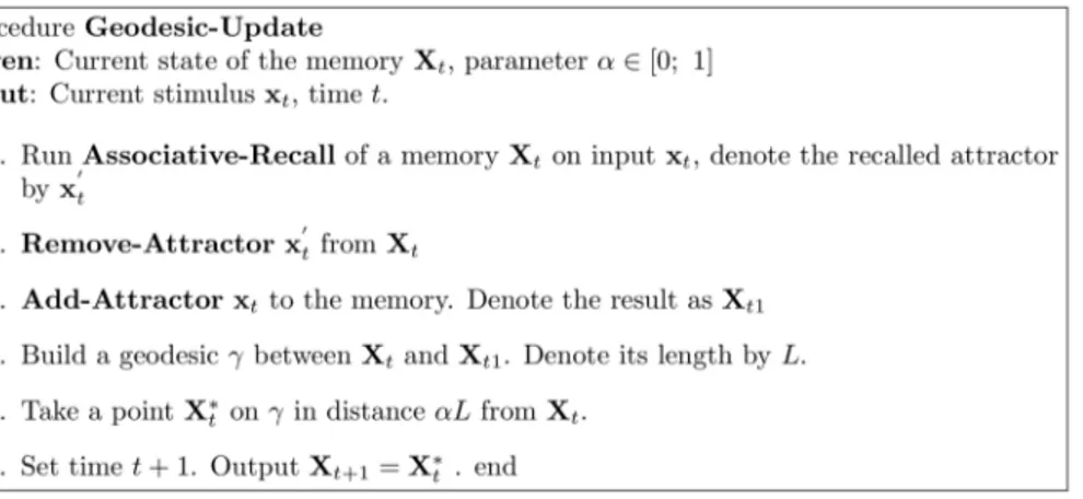
The global geodesic ReC Algorithm. We propose a memory update algorithm that assumes that every ReC update has a global effect. Mathematically it is based on geodesic computation in the Reimannian manifold representing the memory attractors. The metric structure of this manifold and a comparison with the special case of the Grassmann manifold are derived in Materials and Methods (4.1–4.3).
Suppose that we have an initial memoryXt that containsm patterns (concepts) xt,1,xt,2,. . .,xt,m. We then obtain Xt1 by replacing one of the attractor patternsx’twith a new stimulusxt that recalls it. The distance betweenXtandXt1can be interpreted as a measure of the amount of ‘‘surprise’’ that the memory experiences when it meets a new stimuli. To track these changes, we build a geodesiccXt1
Xt joiningXtandXt1on the manifold and take a new point Xt~cXt1
Xt (a). Here a
[½0,1is a step parameter related to the size of a shift during each update. Whena~0, the memory remains atXt, when a= 1, the memory is changed to
Xt1.
Using the same process, when a stimulusxtz1appears we can track the change fromXtz1toXtz2. The process the continues for future stimuli. The algorithm of memory update using geodesics is shown in Fig. 1. The exact geodesic calculation is described in the Materials and Methods. Its complexity depends on the optimiza-tion algorithm used. The dimension of our manifold isd~O(mn). A ‘‘typical’’ gradient calculation would requireO(d2)operations. The gradient-like minimum search calculation has complexity
O(d2=e) where e is the required tolerance [28]. This leads to complexity O((mn)2=e) [29]. However, with derivation-free optimization techniques which do not require explicit gradient calculations, we can reduce this complexity estimation toO(mn=e). The Local Approximate ReC Algorithm. The exact computation of geodesics may be resource consuming especially for high dimensional data. Here we develop a simplified ReC algorithm with local rather than global updates to attractors. In this linear approximation, we simply replace the geodesic with a straight line in the coordinate space.
This leads to the Approximate-Update algorithm in Fig. 2. The approximation algorithm’s complexity isO(mn), equivalent to the
derivative-free version of the geodesic algorithm. However, the approximation algorithm is much easier and faster to implement. Because it requires only a few operations per element, the complexity does not depend on the tolerance.
While the approximate algorithm of Fig. 2 shows only one update per reconsolidation, we can easily construct a version of this algorithm that updates any desired number of attractors. For this, we repeat step 3 for thek most relevant attractors with the largest values offjwherez~S
{1z, and use the valuea
j~afjfor thej-th attractor. This version of the algorithm demonstrates gang effect properties by updating neighboring attractors.
The approximation error is bounded by the following theorem: Theorem 1LetL~r(XI,XF). DenoteXas the solution given by
the geodesic algorithm andXapproxas the solution given by the approximate algorithm. There then exists a constantCsuch that
EX{XapproxEƒCL2
Proof: Let G be a metric tensor on M dependent on coordinates and G0~G(XI). The straight line c
0
between XI andXFis a geodesic in the flat space with a constant metric form G0. SinceMis a twice differentiable manifold,G(X){G0~O(L2) along the geodesiccthat lies betweenXIandXF. Denotesas the distance between the starting pointXIand a given pointXalong the (geodesic) curve.sis called the arc length (see remark 1 below, [30], or other textbook on Riemannian and differential geometry). Becausec0 is a secant of theC2curvecin the coordinate space, whenG(X)~G0, there exists a constantCsuch that for the given arc lengths,Ec(s){c0(s)EƒCs2ƒCL2
Remark 1Arc length could also be defined as a parameterization of a
curvex(s):½0,L?Rnsuch thatVs dx
ds
~1.
Controllable Attraction Radius. As part of the ReKAM architecture we include a mechanism for altering the size of an attractor’s basin of attraction. This affects the probability of recalling an attractor. As the attraction radius goes to zero, the attractor will never be recalled. This is analogous to extinction.
Definition 1A KernelK(u,v)is calleduniformif it depends only on the differenceu{v
If the kernel network has a uniform kernel, Then the attraction radius can be controlled. Assign thescaling factor rk to the k-th attractor. We can then divide thek-th entry ofzbyrkwherezis the temporary vector used in the recall algorithm of ReKAM.
zk~K x{xk
rk
ð4Þ
This causes the attraction basin to be scaled by1=rk.
Model Verification with Human Experiments
We verified our model’s ability to describe reconsolidation by comparing the dynamics of our model to those observed in humans. The first experiment simulates the effect of reconsolida-tion on episodic memories. The second demonstrates the model’s capability to replicate extinction. The third follows memory changes created by the gradual altering of the associated input.
List Learning. We first replicate a human experiment investigating reconsolidation of episodic memories [31]. In the original experiment, participants were split into two groups (A and B). On Day 1, both groups learned a list of 20 objects (List 1) that were associated with a blue basket. On Day 2, Both groups learned a second list of 20 items (List 2). Before learning, group A received a reminder of List 1 in the form of the blue basket; group B did not receive any reminder. On Day 3 both groups were tested on their ability to retrieve List 1. Group A made more errors confusing List 2 items into List 1 than Group B did (Fig. 3). When the experiment
was repeated to test recall of List 2, both groups performed equally well.
In our simulation, all objects were shown as images, rescaled to 320|240pixels. Note that the ability of the model to handle large colored images is already beyond the standard Hopfield model used in previous work. Images were represented as real-valued vectors with componentsx1. . .xn. We added an indicator variable
x0kto each item,x0k[½0,1wherex0k~0denotes that the object is unrelated to the k-th list, and x0k~1 means that the object belongs to this list with 100% certainty.
For computational efficiency, we took the variant of the Gaussian kernel:
K(u,v)~exp {a 2
Xn
k~0
(uk{vk)2{
bn
2
X2
j~0
(u0j{v0j)2
!
ð5Þ
whereaandbare tuned to balance between the data vector and the list indicator components.
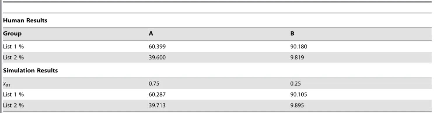
In our simulation we modeled the two groups. For each group we created 40 initial attractors corresponding to the items in both lists. In group A we gradually shifted the value ofx01of each item towards 1 when this item was recalled with the blue basket reminder in the background to simulate the effects of reconsolida-tion. In group B, these updates were not performed. For both groups we tested the memory in recall mode inputting 1000 new vectors per list by taking the attractor and adding uncorrelated white noise (intensity equaled 10% of data STD). For all query vectors, we set thex01~0:5as the initial value.
Using our model, we found an exact correspondence between our simulation and the human experiment for values ofx01~0:75 for Group A andx01~0:25for Group B (see Table 1).
We next simulated more values of x01 which could arise for varying levels of reconsolidation due to differing experimental procedures, memory type, etc. (Fig. 4).
Extinction. Many recent experiments have demonstrated the effects of fear extinction in both humans and animals – e.g. [32], [33], [34]. Numerical simulations with Hopfield memory and Hebbian-like learning were presented in [25]. Our model has a far larger number of far more detailed memories than previously modeled.
We propose to model extinction as a reduction in the attractor’s radius. To demonstrate, we created a kernel network that memorized 10 images. All images were scaled to320|240pixels. One of the images was randomly chosen to be a ‘‘fear’’ (shock) memory. In our procedure, the scaling factor for the ‘‘shock’’ attractor was gradually decreased. This process is analogous to the weakening of the memory occurring through reconsolidation during extinction training. For each scaling factor value we Figure 2. Algorithm of Approximate Update.
doi:10.1371/journal.pone.0068189.g002
Figure 3. Results of the original list learning human experiment [31]. Group A received a reminder cue before learning List 2. This resulted in the List 1 memory becoming labile and updated by integrating some of the new items from List 2. Group B did not receive this reminder and these intrusions were not seen. For our analysis, results were normalized for each group by dividing the number of items recalled per list by the total number of items recalled in both lists together.
measured the frequency of retrieval (recall) of the shock memory on 1000 random inputs (Fig. 5). The decreasing attraction basin radius effectively extinguishes the fear memory trace as its probability of recall goes virtually to 0.
Updating Memories Incrementally. In an experiment testing the incremental changes of gradually morphing memories [35], participants learned to recognize four faces as ‘‘friends.’’ One face was morphed incrementally over a period of days. When the face morphed slowly, participants continually recognized the morphed face as their original friend. By the end of the process, the morphed face was recognized as a friend while the original face was not. The results demonstrated merging of the source and the new face. However, this effect was only observed when the faces were changed gradually, demonstrating that the order in which morphing took place was crucial. A gradual, subtle change was needed to allow for reconsolidation to occur.
In our previous work [17] we published a numerical experiment with morphing face images that replicated the previous result described above. Attractors in the KAM were gradually morphed following the slowly changing face inputs.
Here we present a similar experiment aimed at examining the network’s ability to track images varying gradually over time. Additionally, we compare the performance of the exact and approximate ReC algorithms for this manipulation. We created a training set consisting of 9,000 rotated digits. The rotated digits were created from 100 original MNIST handwritten digits (10 per class from ‘0’ to ‘9’). Digits were28|28 pixel grayscale images which we rotated counterclockwise from0oto180o(Fig. 6).
We applied principal-component (PC) preprocessing without considering any specific handwritten digit optimized feature extraction techniques. We took the first d~200 PCs which contain 96.77% of the variance. For computational efficiency, the kernel we chose was:
K(x,y)~exp {a 2R2
Xd
k~1
wk(xk{yk)2
!
ð6Þ
whereR2~Xd
k~1
wk, andais a bias parameter. This is a Gaussian
kernel dependent on a weighting metric. The weights were chosen as:
wk~
STD(xk)
1
Q XQ
l~1
STDl(xk) {1
0
B B B B @
1
C C C C A
2
ð7Þ
We also tried:
wk~ 1
K XK
l~1
(Elxk{Exk)2 ð8Þ
WhereEl andSTDl are the expectation and standard deviation over thel-th class, and Q is the number of classes. Formula (7) yielded better results.
Evolution of the classification rate over time for the digit rotation experiment is shown in Fig. 7 with confusion matrices in Fig. 7. The exact reconsolidation algorithm achieved a recognition accuracy of 96.4+/20.43%. Results for the local approximate
algorithm were 96.32+/20.26%. The algorithm without
reconso-lidation performed significantly worse (see Fig. 7). The CPU time was 142 sec for the approximate algorithm and 54.7 min for the exact geodesic reconsolidation on Intel Centrino Duo 1.4 GHz CPU with no parallelism, in the Matlab environment. The average
relative error in attractors was
xexact{xapprox
=kxexactk&1:44:10{2.
When inputs were shuffled randomly, gradual reconsolidation was unable to occur. We note that because we are testing on a handwritten digit dataset, there are variations between each test digit: while an ideal number 6 rotated1800would be equal to an
ideal number 9, this will very rarely be the case with the variable hand written digits. Results of no reconsolidation for digits rotated at1800(Fig. 8–C) shows that digits such as 0, 1, and 8 remain
mislabeled while, to a human eye, these would seem the same. It is possible that using a preprocessing technique specifically designed for hand written digit recognition may allow the system to Figure 4. Results of our models simulation of reconsolidation
on the list learning experiment for different values of the reconsolidated parameter x01. x01~0:75 and x01~0:25 exactly matched the results of Group A and Group B of the human experiment.
doi:10.1371/journal.pone.0068189.g004
Figure 5. Results of extinction experiment showing the probability of shock memory retrieval as the attraction radius multiplier is varied. Each point represents the average of 1000 random input trials as well as their standard deviation. Note that the scale of the x-axis varies.
generalize these specific cases to a greater degree. However, even under these conditions, the reconsolidation algorithm works effectively and allows for accurate classification under constantly changing inputs.
Continuous-time ReKAM Models Firing-Rate Dynamics
Up to here, we described the discrete-time form of associative recall. We next relate the ReKAM to biology by introducing a continuous-time version of the kernel memory and comparing it to other firing-rate models. It is important to note that the nature of the time (discrete or continuous) is involved only in dynamical systems of recall, not in the reconsolidation phase. Any step of the reconsolidation (both exact and approximate) depends only on the input and the attractors, not on the time. For this reason both the exact and approximate algorithms of ReC work in continuous time.
The Hopfield equation for thei-th neuron is:
dxi
dt ~{lixizf XN
j~1
wijxjzIi
!
ð9Þ
wherexiis the output of thei-th neuron,wijare the elements of
the symmetric synaptic matrixW,Iiare direct external inputs,f is the activation function, andliis the ‘‘relaxation rate’’ of thei-th neuron. The Hopfield equation (9) imposes linear and symmetric neuron-to-neuron interactions in the network which can be described by the synaptic matrixW. Escalating the model from discrete neurons to neural field (mean field) gives rise to the Wilson-Cowan partial integro-differential equation [36]:
Lu
Lt~{luzf ð
D
w(x,y)u(y)dyzI(x)
0
@
1
A ð10Þ
If the activation function is simply the Heaviside step function, equation (10) becomes the Amari field equation [37].
If the network’s activity is a Markov stochastic process (with a vectorx), then the first-order approximation of the average firing rate dynamics is (see [38]):
Figure 6. Example of rotated digit inputs (A) and corresponding attractors (B) during reconsolidation. doi:10.1371/journal.pone.0068189.g006
Table 1.Comparing the results of actual human experiment to our model’s simulation.
Human Results
Group A B
List 1 % 60.399 90.180
List 2 % 39.600 9.819
Simulation Results
x01 0.75 0.25
List 1 % 60.287 90.105
List 2 % 39.713 9.895
dxi
dt ~{lxizFiðx,IÞ: ð11Þ
This equation can have arbitrary dynamics in contrast to (9) that has a Lyapunov function and converges to attractors.
We propose a continuous-time version of the Kernel Associative Memory that updates the recall similar to (11):
dxi
dt ~{lxizfi XS
{1zzI
ð12Þ
where the components ofzare:
zi~K(xi,x):
i~1. . .m ð13Þ
The continuous ReKAM described by Equations (12) – (13) with a scalar-product kernel is isomorphic to (9) except for having the synaptic matrix W calculated by the pseudoinverse rule (not the Hebbian rule), or, equivalently, orthogonal Hopfield learning. This continuous memory inherits the Hopfield-like attractor dynamics but is more biologically relevant: the number of attractors is independent of the input dimension and rewiring of the neurons is dynamic. We propose the continuous ReKAM as a model for firing rate adaptive dynamics in the course of persistent activity in various networks in the brain.
Discussion
While the existence of reconsolidation in human memory was once a topic of debate, the accumulation of human experimental results has led to the mechanism becoming widely accepted in the field of neuroscience. Reconsolidation has been dissociated from extinction learning, the latter of which results in a second memory trace rather than the removal of the old one [39,40]. However, it is not yet entirely clear when or to what extent reconsolidation mechanisms will occur in a given situation. Experimental results have identified numerous boundary conditions involved in
determining whether or not a memory will undergo reconsolida-tion [39,40].
One such boundary condition is the amount of time between a memory’s retrieval and the encountering of relevant stimuli. This time window varies depending on the animal tested [41] and in humans begins about 10 minutes after retrieval and lasts for several hours. During this time, the memory is labile and susceptible to new information or experimental interference. If the stimulus is encountered outside of this time window, reconsolidation will not occur. A second boundary condition is the age and strength of the memory trace, affecting the ease in which the memory will undergo reconsolidation. A stronger or older memory may require longer and more frequent reactivation sessions for reconsolidation to occur. A third condition, the predictability of reactivation stimulus, also plays a role in whether or not reconsolidation will occur. If a subject does not correctly predict a novel response to a stimulus, reconsolidation is more likely to occur in order to update an incorrect prediction model [42]. Another boundary condition is the ‘‘trace dominance’’ – when a memory stabilizes and becomes resistant to reconsolidation and certain amnesic agents.
It would be possible to extend our model in the future to include these observed boundary conditions. The addition of variables that account for time elapsed since retrieval, age of memory, and strength of memory could be implemented to allow for an accurate simulation of the boundary conditions that accompany reconso-lidation. Additionally, a mechanism to account for prediction error would allow for a representation of the novelty prediction that has been shown to influence whether or not reconsolidation will occur. These additions could allow for a more accurate simulation of reconsolidation as well as a more biological learning model.
We have proposed a mathematical framework of memory reconsolidation, which demonstrates properties as seen in human studies: incremental updates, associations, and extinction. Our ReKAM memory model is far more technologically relevant than previous ones in that it is able to include real-valued inputs as well as massively long inputs; the number of memories is independent of input dimension and hence is practically unbounded. This results in a model providing both a better functional understand-ing of reconsolidation and the basis for a powerful technology for following changes in real world environments.
The mathematical structure has its own beauty: The kernel associative memory has an underlying structure of a Grassman-like manifold in the (feature)Q-space. Since it is a curved Riemannian manifold, reconsolidation is no longer a linear update, but the creation of geodesics is required. We provided both an exact Reconsolidation algorithm as well as a more efficient one, which is local in update and does not require the exact computation of geodesics. A continuous time version of the memory is introduced with further biological relevance.
The kernel method opens the door to reconsolidation of multimodal and dynamical (temporal) memories; this is a subject of our future research.
Materials and Methods
Defining a Riemannian Structure for the ReC algorithm
We formulate the distance between two kernel associative networks where both networks have the same kernel and number of memories. Each network contains a different sets of memory attractors. In the Q-space each kernel memory is a symmetric network whose synaptic matrix is a projective operator C:EQ(x)?EQ(x): C2~C. We measure the distance between two projective operators,X and Y (both of finite rankm), as a Figure 7. Results of the digit rotation experiment. The solid lines
show the average accuracy over all classes for rotations between00and
1800. The blue line shows the accuracy while using reconsolidation. The red line shows the corresponding accuracy while not reconsolidating. The dotted lines surrounding the solid lines refer to the standard deviations.
Frobenius norm kX{Ykfro. Taking into account protectiveness and self-conjugatedness ofXandY, we have:
X{Y
k k2fro~tr(X{Y)(X{Y)T~. . .
~tr(XzY{XY{YX)~:::~2(m{trXY)
ð14Þ
For each projective operatorC, the singular value decompo-sition (SVD) leads to the following:
C~VVz
~V(VTV){1VT~
YYT
For anyVdefined as above, a matrixA(m|m) is defined as having elements aij~(vi,vj), the pairwise scalar products of the memorized vectors. In matrix notation this is represented as:
A~VTV
SinceY:EQ(x)?Rmis an orthogonal operator, then
Y~V(VTV){1=2~VA{1=2
Using this template we representXandYas follows:X~WWT,
W=VS{1=2;Y~HHT, andH~WT{1=2. So,
XY~WWTHHT~WS{1=2VWT{1=2HT~WS{1=2Q
xyT{1=2HT,
HereQis anm|mmatrix such thatqxy,ik~K(xi,yj). Having a singular decomposition forXY, we can now compute the distance as
r(X,Y)2~2(m{tr(S{1=2Q xyT
{1=2)): ð15Þ
The above defines a Riemannian structure for the KAM manifold.
Pseudoinverse Memories and the Grassmann Manifold
We next relate the manifold defined by the ReKAM model to the more well-known and less complex Grassmann manifold. An associative memory with a pseudoinverse learning rule is described in [43]. This is a Hopfield-type auto-associative memory defined originally for bipolar vectors: vk[f{1,1gn,k~1. . .m. Suppose these vectors are columns of n|m matrix V. Then a synaptic matrixCof the memory is given by:
C~VVz
ð16Þ
whereVz
is a Moore-Penrose pseudoinverse ofV. For linearly independent columns ofV, the pseudoinverse can be computed by Vz
~(VTV){1VT or by using the Greville formulae (see, e.g., [44]). The resulting weight matrixCis projective, i.e.C2~Cwith rankm.
The Grassmann manifold is a particular type of Riemannian. The Real Grassman manifold is the manifold of allm-dimensional subspaces inRnand is denoted asGn,m. To define the Grassman manifold, we first introduce the Stifiel manifold – a set of orthogonal n|m–matrices Y, YTY~Im endowed with the Riemannian metric which is induced by the Euclidean norm in Figure 8. Confusion matrices for rotating digit experiment showing predicted labels vs true labels where a correct classification appears along the diagonal.A, B, and C show reconsolidation with00,900, and1800rotations. D, E, and F show results without reconsolidation for
the space of n|m-matrices. Next, we say that two matrices are equivalent if their columns span the same m-dimensional subspace. This means that two matricesYandY0 are equivalent if they are related by right multiplication of an orthogonalm|m
matrix U: Y0~YU. The quotient of the Stiefel manifold with respect to this equivalence relation is called Grassmann Manifold [45].
For eachm-dimensional subspace inRn there exists a unique projective matrixCof rankm, and vice versa (see [46]). Therefore a space ofm-ranked projective matrices is a Grassmann manifold
Gn,m. Moreover, the Frobenius norm of the difference of two projective matrices EX{YEfro gives one possible Riemannian metric over this manifold.
The Grassman manifold emerges in our model in the special case of a scalar-product kernel. Other kernels used in our ReKAM model result in manifolds that can be considered generalizations of the Grassmann.
Computing Geodesics for the ReC Algorithm
To implement the geodesic update algorithm, we have to efficiently compute geodesics on the kernel memory manifolds. Given the metric in explicit form (15) this can be solved as an optimization problem. Let x1 and x2 be points on manifoldM with metric r. Let a point x lie on the (minimizing) geodesic segment joiningx1and x2.xdivides the segment into two parts with proportions a:1{a. Let x’ be a point which lies on the manifold but not in the geodesics. The process of finding x is stated as follows:
r(x0,x)zr(x,x1)?min
r(x0,x)~ar(x0,x1)
ð17Þ
The geodesic minimizes the sum of two distances (first line). For the pointxon the (minimizing) geodesic, the following inequality holds:
r(x0,x)zr(x,x1)ƒr(x0,x0)zr(x0,x1)Vx0[M ð18Þ
The Process (17) can be solved numerically using a Gradient Descent Method (or other first-order unconstrained optimization
method). Its complexity isO(mn=e)for a tolerancee. The constant here is typically large due to the hardness of gradient computation.
Functions with Mercer Condition
The classical KernelsK(x,y)introduced to the field of Machine Learning by Vapnik [26] had the Mercer condition. That is, for all square integrable functionsg(x)the kernel satisfied:
ðð
K(x,y)g(x)g(y)§0: ð19Þ
The Mercer theorem states that if K satisfies the Mercer condition there exists a Hilbert space H with a basis
e1,e2,. . .en. . . and a functionQ:Ex?H,Q(x)~
X ?
k~1
Qkek, where
Q1,Q2. . . :Ex?R, such that
K(u,v)~X
?
n~1
anQn(u)Qn(v) ð20Þ
and allanw0. That is,Kis a scalar product ofQ(u)andQ(v) General Mercer kernels are not sufficient for creating the associative memory since our kernel memories require that all attractors are linearly independent in the feature space. Some Mercer kernels, such as the basic scalar-product kernel
K(u,v)~vu,vw, do not assure this property. The strong Mercer kernels defined for our kernel memory [17] provide linear independence of the attractors in the feature space which enables correct association.
Acknowledgments
We express our appreciation to Keen Sung for finding and reviewing the relevant literature as well as for helpful discussions and editing advise.
Author Contributions
Conceived and designed the experiments: DN HS PV. Performed the experiments: DN. Analyzed the data: DN PV. Contributed reagents/ materials/analysis tools: DN PV HS. Wrote the paper: DN PV HS. Proved the theorems and derived the algorithms: DN.
References
1. Sara S (2000) Retrieval and reconsolidation: Toward a neurobiology of remembering. Learning and Memory 7: 73–84.
2. Dudai Y (1997) Time to remember. Neuron 18: 179–182.
3. Eichenbaum H (2006) The secret life of memories. Neuron 50: 350–352. 4. Dudai Y, Eisenberg M (2004) Rite of passage of the engram: Reconsolidation
and the lingering consolidation hypothesis. Neuron 44: 93–100.
5. Nader K, Schafe G, LeDoux J (2000) Fear memories require protein synthesis in the amygdala for reconsolidation after retrieval. Nature 406: 722–726. 6. Lee J, Everitt B, Thomas K (2004) Independent cellular processes for
hippocampal memory consolidation and reconsolidation. Science 304: 839–843. 7. Medina J, Bekinschtein P, Cammarota M, Izquierdo I (2008) Do memories consolidate to persist or do they persist to consolidate? Behavioural Brain Research : 61–69.
8. Antoine B, Jocelyne C, Serge L (2012) Reconsolidation of memory: a decade of debate. Progress in Neurobiology.
9. Golkar A, Bellander M, Olsson A, Ohman A (2012) Are fear memories erasable?–reconsolidation of learned fear with fear-relevant and fear-irrelevant stimuli. Frontiers in Behavioral Neuroscience 6.
10. Barlow D (2004) Anxiety and its disorders: The nature and treatment of anxiety and panic. Guilford Press.
11. Rescorla R (2004) Spontaneous recovery. Learning and Memory 11: 501–509. 12. Nader K (2003) Memory traces unbound. Trends in Neurosciences 26: 65–72.
13. Alberini C (2005) Mechanisms of memory stabilization: are consolidation and reconsolidation similar or distinct processes? Trends in neurosciences 28: 51–56. 14. Schiller D, Monfils M, Raio C, Johnson D, LeDoux J, et al. (2009) Preventing the return of fear in humans using reconsolidation update mechanisms. Nature 463: 49–53.
15. Agren T, Engman J, Frick A, Bjorkstrand J, Larsson E, et al. (2012) Disruption of reconsolidation erases a fear memory trace in the human amygdala. Science 337: 1550–1552.
16. Nowicki D, Siegelmann H (2009) The secret life of kernels: Reconsolidation in exible memories. In: Frontiers in Systems Neuroscience. Conference Abstract: C o m p u t a t i o n a l a n d s y s t e m s n e u r o s c i e n c e . d o i : 1 0 . 3 3 8 9 / c o n -f.neuro.06.2009.03.271.
17. Nowicki D, Siegelmann H (2010) Flexible kernel memory. PLoS ONE 5: e10955.
18. Wills T, Lever C, Cacucci F, Burgess N, O’Keefe J (2005) Attractor dynamics in the hippocampal representation of the local environment. Science 308: 873–876. 19. McClelland J, Rumelhart D (1981) An interactive activation model of context effects in letter perception: Part i. an account of basic findings. Psychological Review 88: 375–407.
20. Hopfield J (1984) Neurons with graded response have collective computational properties like those of two-state neurons. PNAS 81: 3088–3092.
22. Maass W, Joshi P, Sontag E (2007) Computational aspects of feedback in neural circuits. PLOS Computational Biology 3.
23. Blumenfeld B, Preminger S, Sagi D, Tsodyks M (2006) Dynamics of memory representations in networks with novelty-facilitated synaptic plasticity. Neuron 52: 383–394.
24. Siegelmann H (2008) Analog-symbolic memory that tracks via reconsolidation. Physica D 237: 1207–1214.
25. Osan R, Tort A, Amaral O (2011) A mismatch-based model for memory reconsolidation and extinction in attractor networks. PLoS ONE 6: e23113. 26. Vapnik V (1998) Statistical Learning Theory. John Wiley & Sons, NY. 27. Ben-Hur A, Horn D, Siegelmann H, Vapnik V (2001) Support vector clustering.
Journal of Machine Learning Research 2: 125–137.
28. Nocedal J, Wright S (2006) Numerical optimization. Springer Science+Business Media.
29. Udriste C (1994) Convex functions and optimization methods on Riemannian manifolds, volume 297. Springer.
30. do Carmo M (1992) Riemannian Geometry. Birkhauser Verlag AG. 31. Hupbach A, Gomez R, Hardt O, Nadel L (2007) Reconsolidation of episodic
memories: A subtle reminder triggers integration of new information. Learning & Memory 14: 47–53.
32. Monfils M, Cowansage K, Klann E, LeDoux J (2009) Extinction-reconsolidation boundaries: key to persistent attenuation of fear memories. Science 324: 951– 955.
33. Suzuki A, Josselyn S, Frankland, Paul W, Masushige S, et al. (2004) Memory reconsolidation and extinction have distinct temporal and biochemical signatures. The Journal of neuroscience 24: 4787–4795.
34. Pedreira M, Pe´rez-Cuesta L, Maldonado H (2004) Mismatch between what is expected and what actually occurs triggers memory reconsolidation or extinction. Learning & Memory 11: 579–585.
35. Preminger S, Blumenfeld B, Tsodyks DSM (2009) Mapping dynamic memories of gradually changing objects. Proceedings of the National Academy of Sciences 106: 5371–5376.
36. Wilson H, Cowan J (1973) A mathematical theory of the functional dynamics of cortical and thalamic nervous tissue. Kybernetik 13: 55–80.
37. Amari S (1977) Dynamics of pattern formation in lateral-inhibition type neural fields. Biol Cybernet 27: 77–87.
38. Buice M, Cowan JD, Chow C (2009) Systematic uctuation expansion for neural network activity equations. arxivorg arXiv:0902.3925v2.
39. Besnard S, Machado ML, Vignaux G, Boulouard M, Coquerel A, et al. (2012) Influence of vestibular input on spatial and nonspatial memory and on hippocampal nmda receptors. Hippocampus 22: 814–826.
40. Besnard A (2012) A model of hippocampal competition between new learning and memory updating. The Journal of Neuroscience 32: 3281–3283. 41. Tronson N, Taylor J (2007) Molecular mechanisms of memory reconsolidation.
Nature Reviews Neuroscience 8: 262–275.
42. Sevenster D, Beckers T, Kindt M (2012) Retrieval per se is not sufficient to trigger reconsolidation of human fear memory. Neurobiology of learning and memory 97: 338–345.
43. Personnaz L, Dreyfus I (1986) Collective computational properties of neural networks: New learning mechanisms. Phys Rev A 34: 4217–4228.
44. Albert A (1972) Regression and the Moore-Penrose pseudoinverse. Academic Press, NY-London.
45. Absil P, Mahony R, Sepulchre R (2004) Riemannian geometry of grassmann manifolds with a view on algorithmic computation. Acta Applicandae Mathematicae 80: 199–220.