Modeling the angular dependence of satellite retrieved Land Surface Temperature (LST)

(1)

UNIVERSIDADE DE LISBOA

FACULDADE DE CIÊNCIAS

DEPARTAMENTO DE ENGENHARIA GEOGRÁFICA, GEOFÍSICA E ENERGIA

Modeling the angular dependence of satellite retrieved

Land Surface Temperature (LST)

Sofia Nunes Lorena Ermida

Dissertação

Mestrado em Ciências Geofísicas

Especialização em Meteorologia

(2)

(3)

UNIVERSIDADE DE LISBOA

FACULDADE DE CIÊNCIAS

DEPARTAMENTO DE ENGENHARIA GEOGRÁFICA, GEOFÍSICA E ENERGIA

Modeling the angular dependence of satellite retrieved

Land Surface Temperature (LST)

Sofia Nunes Lorena Ermida

Dissertação

Mestrado em Ciências Geofísicas

Especialização em Meteorologia

Dissertação orientada por

Doutora Isabel Trigo e Prof. Doutor Carlos da Camara

(4)

(5)

Acknowledgments

I would like to thank to Isabel Trigo and Carlos da Camara for their guidance and support during my scientific research.

I am indebted to Folkie Olesen and Frank Göettsche for providing the in situ data at the Évora site. My research was funded by a scholarship within the framework of LSA-SAF, an R&D project co-funded by EUMETSAT.

(6)

(7)

Abstract

Satellite retrieved values of Land Surface Temperature (LST) over heterogeneous pixels generally depend on viewing and illumination angles as well as on the characteristics of the land cover. A geometrical model is presented that allows estimating LST of a given pixel for any viewing and illumination angles. The Boolean scene model is used to estimate the per-pixel fractions covered by the following three scene components: sunlit background, shaded background and vegetation. Estimates of the average area covered by canopies and by shadow are derived from the projection of a single arbitrarily-shaped vegetation element (e.g. ellipsoidal or conical tree canopies) onto a fine scale regular grid.

The model is applied to time-series of continuous in situ brightness temperature measurements as obtained at the LSA-SAF validation site in Évora (Portugal) during 2011 and 2012. Measurements are performed every minute by four radiometers, two of them observing the sunlit background and the other two a tree crown and the sky at 53° zenith angle. It is assumed that the shadow temperature is determined by daily maxima of air and sunlit background temperatures.

The resulting composite temperature is compared against LSA-SAF operational LST data as retrieved from the SEVIRI instrument on-board Meteosat-8. Results show a bias of order of 1 K and a RMSE of about 1.5K. LST data are also compared against MODIS (level 3) daily LST. The LST difference between MSG and MODIS shows a strong dependence on viewing geometry that suggests relying on the geometrical model to generate estimates of LST differences between the two sensors.Results obtained with the model reveal a significant decreasing of the standard deviation error between the sensors.

Key-words: Land Surface Temperature; geometric effects; Meteosat Second Generation; LST

validation; land surface anisotropy

Resumo

A temperatura de superfície do solo (Land Surface Temperature - LST) é definida como a temperatura radiométrica da superfície sobre terra, correspondendo à radiação emitida no infravermelho (IV) térmico por uma camada com espessura da ordem da profundidade de penetração da radiação IV, da ordem do comprimento de onda. A LST é uma variável climatológica importante e, também, um parâmetro de diagnóstico das condições da superfície do solo. Pode ser utilizada para estimar fluxos de calor sensível à superfície, a humidade do solo, a evapotranspiração e propriedades da vegetação, incluindo o seu stress hídrico.

A deteção remota, nomeadamente a efetuada através de satélites, constitui o único meio disponível para a obtenção de LST a uma escala espacial global e regular e com elevada frequência temporal. A

Land Surface Analysis Satellite Application Facility (LSA-SAF) dissemina, de forma operacional e em

tempo quase real, um produto de LST obtido por aplicação de um algoritmo do tipo “generalized split-window” a observações de temperatura de brilho no topo da atmosfera efetuadas pelo Spinning

Enhanced Visible and InfraRed Imager (SEVIRI) a bordo dos satélites da série Meteosat Second Generation (MSG).

A validação da LST da LSA-SAF envolve não só a sua comparação com medições in situ mas também com a LST obtida por sensores a bordo de outros satélites. As principais fontes de discrepâncias de LST entre satélites são: 1) a calibração do sensor, 2) as funções de resposta, 3) a resolução espacial e temporal, 4) a correção atmosférica aplicada, 5) as estimativas de emissividade de superfície adotadas, 6) a máscara de nuvens utilizadas e 7) a anisotropia angular. Destas, a sensibilidade da LST à anisotropia angular é um dos tópicos menos estudados. No entanto, os produtos de satélite de LST são, em geral, variáveis direcionais, isto é, a LST obtida para uma dada cena, utilizando o mesmo sensor, mas com ângulos de visão diferentes, frequentemente apresenta valores diferentes, dependendo de fatores como o tipo de superfície, as características do solo e a inclinação do terreno. A estrutura da superfície tem uma influência importante na temperatura, devido particularmente a efeitos de sombreamento pelos elementos de vegetação e inclinação do terreno que resultam numa dependência da LST dos ângulos zenital e azimutal de visão. Para superfícies homogéneas, a variabilidade da LST

(8)

é essencialmente função da direccionalidade da emissividade, enquanto para superfícies heterogéneas a variabilidade angular está na sua maioria associada às proporções observadas pelo satélite de diferentes componentes que possuem as suas próprias temperatura e emissividade.

Existem diversos modelos de transferência radiativa que tratam de diferentes formas a anisotropia da radiação em zonas vegetadas. Os modelos Ótico-Geométricos foram desenvolvidos em particular para descrever florestas e outros cobertos vegetais descontínuos. Estes modelos operam assumindo que a copa da vegetação pode ser descrita por objetos geométricos distribuídos espacialmente de acordo com determinado modelo estatístico. A interseção e reflecção de luz são calculadas analiticamente a partir de considerações geométricas. Nestes modelos a radiância de uma dada região é estimada como sendo uma média pesada das radiâncias de cada componente básico (normalmente, o solo ao sol e à sombra e a copa ao sol e à sombra).

Neste estudo apresenta-se um modelo geométrico que permite estimar as áreas projetadas de cada componente utilizando geometria de raios paralelos para descrever a iluminação de um único elemento de vegetação tridimensional e a sombra que origina. Dada a forma e tamanho do elemento de vegetação e a geometria de visão e iluminação, as diferentes proporções podem ser estimadas recorrendo ao formalismo do modelo Booleano, desde que se possa assumir que os objetos possuem uma distribuição espacial aleatória. O modelo Booleano inclui ainda a possibilidade de sombreamento mútuo entre objetos e a sobreposição de copas.

Este tipo de modelo ótico-geométrico tem sido bastante utilizado por vários autores em estudos de anisotropia de temperatura da superfície. O procedimento proposto no presente trabalho tem a vantagem de recorrer a um método computacional simples para calcular as projeções, em vez de utilizar um método analítico mais rígido e complexo. O método consiste em projetar um elemento de vegetação tridimensional (copa elipsoidal ou cónica) numa malha de elevada resolução, o que permite a utilização de qualquer forma e tamanho para a vegetação e até mesmo a combinação de diferentes formas e tamanhos.

As radiâncias das componentes são obtidas a partir de medições in situ da temperatura de brilho provenientes da estação de validação de LSA-SAF em Évora. Estas medições são efetuadas a cada minuto por quatro radiómetros que observam o solo ao sol (em dois pontos diferentes), a copa de uma árvore e o céu a um ângulo zenital de 53º, sendo a última medição utilizada para estimar a componente de fluxo radiativo descendente refletido. Assume-se ainda que a temperatura da sombra é determinada pelos valores máximos diários das temperaturas do ar e do solo ao sol. O modelo é posteriormente aplicado ao pixel do MSG que contém a estação de Évora, utilizando-se informação de terreno sobre a densidade de árvores e a sua forma e tamanho médios.

A temperatura do compósito resultante da combinação do modelo geométrico e das medições in situ é então comparada com a LST operacional disseminada pela LSA-SAF. Os resultados mostram uma boa concordância entre a temperatura do compósito e a LST, apresentando um viés de cerca de 1ºC e um erro médio quadrático de cerca de 1.5ºC. Acresce que os resultados mostram que existe um impacto significativo de heterogeneidades da superfície na LST e, especialmente, que esse impacto varia ao longo do dia e do ano uma vez que depende das temperaturas relativas do solo ao sol e à sombra e da copa. Em relação a outros estudos efetuados, o presente trabalho proporciona uma avaliação mais pormenorizada deste efeito, em particular graças à análise efetuada a uma grande variedade de ângulos de visão e iluminação, emissividades de superfície e coberto vegetal.

A simplicidade do modelo permite a sua aplicação a qualquer satélite, geoestacionário ou de orbita polar. A LST foi, assim, igualmente comparada com o respetivo produto do sensor MODIS. A comparação dos dois produtos mostra a presença de um viés e de um desvio padrão dos erros de cerca de 3ºC. O modelo geométrico foi mais uma vez aplicado às medições in situ, de forma a estimar e corrigir desvios entre as estimativas de LST com base nos dois sensores, que estão associados a geometrias de visão diferentes. A aplicação desta correção resulta numa redução significativa do desvio padrão dos erros, resultado este expectável, dada a geometria de visão variável do MODIS. Quanto ao viés observado entre os dois sensores, este não pode ser atribuído a diferenças na geometria de visão, estando provavelmente relacionado com outras fontes persistentes de erro. As diferenças observadas podem eventualmente ser atribuídas às discrepâncias significativas observadas entre as emissividades utilizadas pela LSA-SAF e pelo MODIS. Com efeito, no período de estudo, as diferenças variam entre 0.005 e 0.01, com o MODIS a apresentar sempre valores mais elevados, facto consistente com o viés negativo observado.

(9)

Os resultados obtidos sugerem que o procedimento proposto pode constituir uma ferramenta útil para a validação e comparação de LST de diferentes sensores. O modelo geométrico apresentado representa um ponto de partida para a compreensão dos efeitos direcionais na LST. Pode antecipar-se que este modelo virá a ser utilizado num estudo alargado de sensibilidade, a ser realizado para todo o disco MSG – e por isso para uma vasta variedade de tipos de superfície e geometrias de visão e iluminação – de modo a que sejam identificadas áreas e períodos do dia e do ano em que estes efeitos são mais pronunciados.

Palavras-chave:

Temperatura de superfície; efeitos geométricos; Meteosat Second Generation; validação de LST; anisotropia em superfícies continentais

(10)

(11)

1. Introduction

Land Surface Temperature (LST) is defined as the “skin” temperature of the earth’s surface over land. The term “skin” is used as LST relates to the radiation emitted in the thermal infrared from a layer of the order of the penetration depth, i.e, of the considered wavelength (Norman and Becker, 1995). LST is an important climatological variable (Sellers et al, 1992) as well as a diagnostic parameter of land surface conditions. It can be used to estimate surface heat fluxes (Mannstein, 1987; Caparrini et al, 2004), soil moisture (Carlson, 1986; Nemani et al, 1993), evapotranspiration (Kustas and Norman, 1996) and vegetation properties (Lambin and Ehrlich, 1997), including vegetation hydric stress (Jackson et al, 1981).

Remote sensing is the only available method that allows retrieving LST on a global spatially distributed scale and on a regular basis. The Land Surface Analysis Satellite Application Facility (LSA-SAF) provides a LST product (Trigo et al, 2011) as obtained through the application of a generalized split-window algorithm (Madeira, 2002) to the data from the Spinning Enhanced Visible and InfraRed Imager (SEVIRI) on board Meteosat Second Generation (MSG) satellites.

The validation of the LSA-SAF LST involves its comparison with LST either as obtained from sensors on-board other platforms, or by in situ measurements (Trigo et al, 2008). The main sources of LST differences between sensors are (1) sensor calibration, (2) filter response functions, (3) temporal and spatial resolutions, (4) atmospheric correction, (5) surface emissivity assumptions, (6) cloud mask, (7) angular anisotropy (Barroso et al, 2005). The sensitivity of LST to angular anisotropy is the least studied one. Nevertheless, satellite LST products are usually directional variables, i.e., hypothetical LST retrievals obtained for the same scene, using the same sensor, but with different view angles would likely produce different temperature values, depending on factors such as surface type, soil characteristics and slope orientation relative to sun. Surface structure exerts an important role on the temperature, due in particular to shadowing effects that result in a dependence of LST on the zenithal and azimuthal view angles. For flat homogeneous surfaces, the variability in LST is mainly a function of directional emissivity (Dash et al, 2002), whereas for heterogeneous surfaces the angular variability is mostly associated to areal proportions of different components that have individual temperatures and emissivities.

There are several types of radiative-transfer models that treat in different ways the anisotropy of radiation in canopies. An overview is given in Jones and Vaughan (2010) that provides examples of models that include the Turbid-medium models, the Monte-Carlo ray-tracing models, the radiosity models, the Kernel-driven models and the Geometrical-optical models. Models of the latter type have been developed particularly to describe forests and other discontinuous canopies. They operate by assuming that the canopy may be described by an array of geometrical objects arranged in space according to some statistical distribution. The light interception and reflection is computed analytically

(14)

2 Sofia Ermida

from geometrical considerations. For these models, the overall radiance at any angle is calculated as a weighted average of the radiances from each component (usually, sunlit and shaded background and sunlit and shaded canopy).

This study presents a geometric model that allows estimating the projected areas of the different components using parallel-ray geometry to describe the illumination of a three-dimensional vegetation element and the shadow it casts. As discussed in Strahler and Jupp (1990), if the size and shape of the vegetation elements are fixed, if the viewing and illumination geometries are kept constant, and if object centers are considered to be randomly distributed, then their proportions may be estimated using the so-called Boolean model of Serra (1982). This formulation includes the possibility of mutual shadowing between objects and crown overlapping.

This type of geometric-optical model has been used by several authors to solve radiative transfer problems associated to surface heterogeneities related to vegetation (Li and Strahler, 1986; Franklin and Strahler, 1988; Strahler and Jupp, 1990; Li and Strahler, 1992; Lagouarde et al, 1995; Ni et al, 1999), as well as in studies of surface temperature anisotropy (Minnis and Khaiyer, 2000; Pinheiro et al, 2006; Rasmussen et al, 2010). Instead of relying on a more rigid analytical approach, the procedure proposed in this work presents the advantage of using a simple computational method to calculate the geometrical projections, with very few a priori conditions. The method consists in projecting a three-dimensional vegetation object onto a fine grid, which allows the use of any vegetation shape and size or the combination of different shapes and sizes.

Radiances are obtained from in situ measurements of brightness temperature from the LSA-SAF validation site in Évora (Portugal). The model is then applied to the MSG pixel containing the Évora site, using ground information on tree density and average tree shape and size.

The LSA-SAF LST is also compared against the equivalent MODerate resolution Imaging Spectroradiometer (MODIS) product. The Geometric Model combined with in situ measurements is finally used to estimate and remove LST differences between MSG and MODIS associated to viewing geometry and surface heterogeneities.

2. Data and Methods

2.1 Satellite Data

2.1.1 MSG/SEVIRI

The LSA-SAF produces the LST product at full spatial and temporal resolution based on the MSG/SEVIRI data, namely with a 15 minute sampling and a spatial resolution of 3km at the sub-satellite point, which degrades with increasing distance from nadir, reaching about 5km over

(15)

South-Modeling the angular dependence of satellite retrieved Land Surface Temperature (LST)

Sofia Ermida 3

Western Europe. The product is available for all land pixels within the Meteosat disk, which have viewing zenith angle lower than 70º.

This study was performed for the MSG pixel containing the Évora validation site (38.45ºN, 8.00ºW; Southern Portugal). Sampling time was corrected for scanning delays, which for Évora corresponds to adding 10 minute to the nominal image time. This value was estimated taking into account that the scanning by SEVIRI is from east to west and south to north (Schmetz et al, 2002).

2.1.2 MODIS

The MODIS level 3 daily LST includes four observations, two of them derived from the AQUA sensor (product MYD11A1, version 5) daytime and nighttime observations and the other two derived from the TERRA sensor (product MOD11A1, version 5). Both products include emissivity values used in the LST retrieval for bands 31 and 32 (centered at about 11.03 and 12.02 µm, respectively). Information on geolocation was obtained from MODIS products MOD03 and MYD03, version 5 (http://modis.gsfc.nasa.gov/).

In order to compare MODIS and MSG products, averages were computed of LST values from all 16 MODIS pixels lying within the chosen MSG pixel. Each MODIS observation was matched to the closest MSG time in a 15 minute window. Cloud contamination was avoided by taking into account the MODIS pixels with the highest quality flag. This means that if one of the pixels within the selection has poor confidence level, the observation is rejected. Since MODIS data are provided at local time, this implies adding about 30 minute to match MSG sampling time.

2.2 The Geometric Model

The impact of viewing and illumination geometry on LST retrievals was assessed by means of a geometric model based on the Geometrical-Optical (GO) part of the Geometrical-Optical Radiative Transfer (GORT) model (Ni et al, 1999). The model allows estimating the scene proportions of a given pixel, assuming that the main components are sunlit background, shaded background and canopy. Such geometric-optical thermal radiative transfer models should also differentiate between sunlit and shaded canopy (Jones and Vaughan, 2010), however due to tree capacity to regulate its temperature, temperature differences between the shaded and sunlit parts are expected to be negligible when compared to the differences between sunlit background, shaded background and canopy at the satellite’s pixel scale. It is therefore to be expected that the above mentioned three components should be sufficient to capture the scene angular variability (Pinheiro et al, 2006).

We assume that the pixel’s radiance intercepted by the sensor may be estimated as a linear combination of the radiances emitted by each of the scene components weighted by the respective projected scene fractions. For our purposes we assume that any angular variation in the composite radiance is exclusively due to changes in the scene fractions:

(16)

4 Sofia Ermida

(1)

where is the pixel’s radiance, , and are sunlit background, shaded

background and canopy radiances, respectively, and , and are the respective

component fractions. Each component’s radiance is obtained from in situ measurements of brightness temperature which are converted to radiances using Planck’s Law:

( ( ))

( ⁄ ₎ (2)

where is the Planck constant, is the Boltzmann constant, is the speed of light, is the wavelength and is the brightness temperature. Here we assume that a central wavelength of is representative of the radiometers band that will be used in this study (Göttsche et al, 2013).

The radiance reaching the radiometer is a combination of the radiance emitted and reflected by the surface. The reflected part may be removed using measurements of radiance by a radiometer pointing to the sky ( ):

( ) (3)

where is an effective emissivity that is calculated as a weighted average of the emissivity of

ground and tree components:

( ) (4)

where the Fraction of Vegetation Cover (FVC) is the proportion of surface covered by vegetation. We consider that FVC provides a direct measure of green and non-green proportions of the pixel as seen by a remote sensor. It may be noted that an estimate of the green and non-green proportions based on scene fractions may lead to unrealistic values of emissivity since the ground is usually grassed during winter, changing its emissivity.

The composite radiance is then converted back to temperature using again Planck’s Law:

( )

( ) (5)

2.2.1 The Boolean component

A geometric model was developed to estimate the fractions of sunlit background, shaded background and canopy as seen by the sensor, using information on viewing and illumination geometry, canopy shape and Percentage of Tree Cover (PTC), which is defined as the surface proportion covered by tree crowns.

(17)

Sofia Ermida 5

The geometric model is based on the Boolean Scene Model (Strahler and Jupp, 1990) that shows that the gap probability ( ) between objects within a layer is

( ) ̅( ) (6)

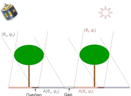
where is the density of object centers, is the viewing zenith angle, is the viewing azimuth angle and ̅( ) is the average area of an object projected at angle ( ) onto the base of the layer. Accordingly, in terms of the geometrical model, ( ) will represent the proportion of background seen from the viewpoint at ( ) when trees have an average areal projection ̅( ) onto the background, and the complement will be the proportion covered by trees (Figure 1). On the other hand, the proportion of non-shaded background will be ( ). However, only a fraction of this, denoted as the proportion ( ) of the background, will actually be visible by the sensor due to overlapping of various scene components within the field of view. Thus, the proportion of illuminated background visible to the viewer will be the joint probability which takes into account the overlapping of the two projections:

sunlit ( ) ( ) { [ ̅( ) ̅( ) ̅overlap]} (7)

The fraction of shaded background is the fraction of seen background that is not illuminated

shaded ( ) sunlit { ̅( )} sunlit (8)

and the fraction of canopy will be

canopy ( ) { ̅( )} (9)

The projected areas ̅( ) are simple to estimate analytically, however the computation of the overlap area may be very complex. We use a projection of a single arbitrarily-shaped vegetation element (an ellipsoidal tree in our case) onto a fine scale regular grid to obtain the projected areas and respective overlap. The tree number density ( _{) is estimated using Percentage of Tree Cover}

(PTC) and the size of tree crown (the average horizontal crown axis R in our case). Assuming random overlap between trees (Liu et al, 2004):

( )

(18)

6 Sofia Ermida

Figure 1 - Schematic representation of projected areas for a given viewing and illumination geometry. The red shaded area is the projection of the trees at the illumination angle ( ), which physically

represents tree shadow. The blue shaded area is the projection of the trees at the viewing angle ( ) which represents the area obscured by tree crown that will not be seen by the sensor. Therefore, the sunlit background as seen by the sensor will be limited to the white area. Part of the

shaded area will be hidden by the crown, corresponding to the overlap area.

2.2.1.1 Input data

The geometric model requires input information on the Percentage of Tree Cover (PTC), Fraction of vegetation cover (FVC) and average tree shape. A value of 0.3 was assigned to PTC based on the percent of tree crowns observed in an IKONOS image (1 m resolution) for an area surrounding the Évora station equivalent to that of a MSG pixel (Trigo et al, 2008). Information on FVC was obtained from the LSA-SAF product Fraction of Vegetation Cover for the pixel containing the Évora site and averaged over each month. The Évora scene was assumed to be composed by trees of ellipsoidal shape with an average canopy horizontal radius R of 5 m, an average canopy vertical radius b of 2.5 m and an average height of crown center H of 6 m.

The model also requires information on both illumination and viewing geometries, namely view zenith angle, view azimuth angle, sun zenith angle and sun azimuth angle. View angles are available for each remote sensor considered, whereas the sun angles may be calculated based on location, date and time of day.

2.3 In situ measurements

The geometric model developed here was applied to time-series of continuous in situ brightness temperature measurements as obtained at the LSA-SAF validation site in Évora (Portugal) from October 2011 to September 2012. Measurements are performed every minute by four radiometers, two of them observing the sunlit background at two different points, a third one observing a tree crown and the last one pointing to the sky at 53° zenith angle, which is used to estimate down-welling reflective

(19)

Sofia Ermida 7

components. The site is particularly appropriated to this study as it corresponds to an area of homogeneous and stable land cover (Quercus woodland).

When comparing the time series of the two radiometers measuring sunlit background temperature at two different points, there is a conspicuous period in the evening for winter months (namely, October to March) where one of the radiometers shows an abnormal deviation (Figure 3).

The periodicity of this contamination suggests it may be due to shadowing of the radiometer field of view, thus corresponding to an incorrect input temperature of the sunlit background component. The other radiometer does not show this contamination but its measurements are not reliable. The team responsible for the maintenance of Évora ground station reported that the grass within the FOV of this radiometer was grazed and no longer represented the surface under canopy in this area. This leads to a change in the surface radiation properties, including a possible decrease in ground emissivity. Even so, this second radiometer may be used to correct the other radiometer’s time series. An analysis of the two time-series showed that they are linearly correlated to a good approximation (Figure 2):

( ) (11)

where parameters and may be estimated using robust regression (Table 1). Using the geometric part of the geometric model, we computed shadow projections for two days with well-defined diurnal cycles. Because the starting and ending times of the shadow contamination are clearly defined for these days, the two to estimate the radiometer’s position relative to the tree (Figure 4-Figure 5). Knowing the radiometer’s position we may automatically select the contaminated part of the time-series and correct it.

(20)

8 Sofia Ermida

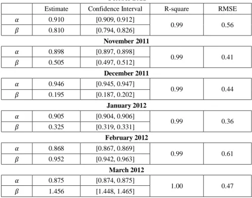
Table 1 – Estimates for parameters and of eq. 11, and the respective 95% confidence intervals, R-square and Root Mean Square Error.

October 2011

Estimate Confidence Interval R-square RMSE 0.910 [0.909, 0.912] 0.99 0.56 0.810 [0.794, 0.826] November 2011 0.898 [0.897, 0.898] 0.99 0.41 0.505 [0.497, 0.512] December 2011 0.946 [0.945, 0.947] 0.99 0.44 0.195 [0.187, 0.202] January 2012 0.905 [0.904, 0.906] 0.99 0.36 0.325 [0.319, 0.331] February 2012 0.868 [0.867, 0.869] 0.99 0.61 0.952 [0.942, 0.963] March 2012 0.875 [0.874, 0.875] 1.00 0.47 1.456 [1.448, 1.465]

Since there is no information available about the shadow temperature, there is the need to have an indirect estimation of it. For this purpose, it is assumed that, for each illumination zenith angle, the shadow temperature is proportional to sunlit temperature, the proportionality constant being determined by the ratio of maximum values of air to sunlit temperatures taken along the considered day. Since the direct incoming radiation is removed from shaded surfaces, we expect their temperature to be close to radiative equilibrium with air. However, air has a different heat capacity and therefore a different response time than that of the ground to net radiation, resulting in a lag of the air diurnal temperature cycle relative to that of the ground (Figure 6). The shadow temperature is accordingly estimated by the following empirical model:

( ) ( ) ( ) (12) where ( ) { ⁄ ⁄ ( ₎ (13)

(21)

Sofia Ermida 9

Figure 3 - Correction of shadow contamination onto the radiometer’s time series. In the upper panels, blue and red curves represent each one of the observed temperature time series by the two radiometers. The black curve represents the obtained time series through regression (eq. 11). The lower panel presents both the corrected and original curves with a

(22)

10 Sofia Ermida

11Feb2012 13:40 11Feb2012 16:20

25Nov2011 13:00 25Nov2011 15:40

Figure 4 – Starting times (left panels) and ending times (right panels) of shadow contamination to the radiometer on the 11th of February 2012 (top panels) and on the 25th of November 2011

(bottom panels). Red dots indicate possible locations for the radiometer on that day.

Figure 5 – As in Figure 4 but with all possible locations merged together which allows estimating the location of the radiometer relative to the tree (black dot).

(23)

Sofia Ermida 11

Figure 6 – Diurnal cycle of air, sunlit and shadow temperatures on the 22th

of February 2012. Air temperature presents a lag relative to the sunlit ground. Shadow temperature is obtained using the

model given by Eq. 12.

3. Results and discussion

3.1 Comparison against LSA-SAF LST data

The composite surface temperature as obtained with our geometric model of viewing and illumination geometries was then used to assess LST satellite estimation corresponding to the pixel containing the Évora site. Results show a RMSE of order of 1 to 2 K throughout the year, the lower values being observed during nighttime. The error standard deviation (STD) is of the same order of magnitude of RMSE whereas the bias presents values between -1 and +1 K. These values suggest that the obtained errors are related to other sources and that the model presents a good agreement with observed LST (Figure 7).

For reference, we also show the comparison between satellite LST and ground composites following the procedure used by Trigo et al. (2008) for LST validation, where the in situ brightness temperature is a “simple composite” of ground observations, i.e. a weighted average of sunlit background and tree crown temperatures, using the Percentage of Tree Cover. In this “simple composite”, neither the daily and seasonal variations in the illumination geometry, nor the actual sensor viewing angle are taken into account.

If we look at the error on an hourly basis it becomes clear that the geometric composition of ground measurements is more important during daytime of the warmer months, i.e. when there is a higher temperature contrast between sunlit and shaded background (Figure 8).

(24)

12 Sofia Ermida

Figure 7 – Monthly daytime (upper panel) and nighttime (lower panel) values of (a) bias, (b) Root Mean Square Error (RMSE) and (c) error Standart Deviation (STD). Error is defined as composite

temperature minus SEVIRI-based LST. The blue line represents the composite of ground observations with geometric model of the surface and the red line represents the “simple

composite” of ground observations. (a)

(b)

(25)

Sofia Ermida 13

Figure 8 – Monthly and hourly bias defined as composite temperature minus SEVIRI-based LST. The upper panel (a) refers to the composite of ground observations with the geometric model of the

surface whereas the lower panel (b) refers to the “simple composite” of ground observations.

3.2 Sensitivity to prescribed parameters

The sensitivity of ground surface temperature composites to values of ground and tree emissivity as well as to Percentage of Tree Cover was evaluated by computing the temperature composites with different values of these parameters. The result was then compared against SEVIRI-based LST.

3.2.1 Tree Emissivity

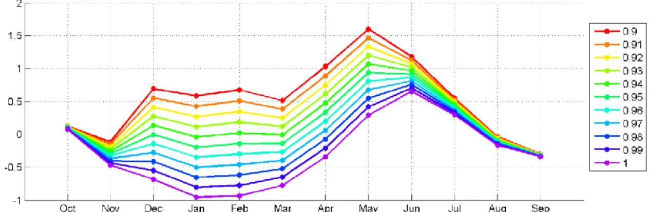
The impact of tree emissivity on the composite temperature has a high seasonal behavior, the impact being particularly high in winter and spring months and negligible in summer and fall (Figure 9). This feature is associated to the intra-annual variability of FVC (Figure 10), where values are extremely low from July to November. It is worth mentioning that the value assigned to tree emissivity at the Évora site is 0.9934, as estimated from lab measurements of tree leaves of the dominant type found around the Évora site.

(a)

(26)

14 Sofia Ermida

Figure 9 – Monthly bias defined as composite temperature minus SEVIRI-based LST, for different values of tree emissivity.

Figure 10 – Monthly mean values of Fraction of Vegetation Cover (FVC) at the Évora site.

3.2.2 Ground Emissivity

The impact of ground emissivity presents a much weaker seasonal behavior, being slightly higher in summer and fall (Figure 11). This feature is also related to the low values of FVC that result in an effective emissivity that is mainly determined by that of the ground. The used ground emissivity value for the Évora site is 0.9689. As in the case of trees, the ground emissivity is obtained from lab measurements respecting to the typical soil types found around the Évora site.

(27)

Sofia Ermida 15

3.2.3 Percentage of Tree Cover

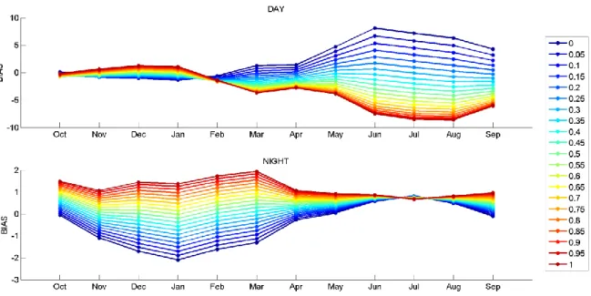
The effect of PTC on composite temperature has a marked intra-annual variability, which presents opposite behavior during day and night (Figure 12). During summer there is a higher impact during daytime which is due to the higher contrast between sunlit ground and tree temperature. During winter, the highest contrast between ground and canopy temperatures tends to occur during night-time: the tree is able to maintain its temperature slightly above that of the ground, particularly under clear sky conditions when it is common to have radiative cooling under very stable conditions. Tree temperature is also closer to air temperature than ground temperature, which often reaches considerably lower values during night. As a consequence, the most pronounced sensitivity to PTC in winter is observed for night-time measurements.

Figure 12 - As in Figure 9 but for percentage of tree cover (PTC), for daytime (upper panel) and nighttime values (lower panel).

3.3 Impact of viewing geometry

The impact of changes in viewing geometry on surface temperature was assessed by making use of the geometric model to compute composite temperature as a function of input view zenith and azimuth angles. Figure 13 and Figure 16 present the temperature deviations from the original temperature field as obtained for the view point of MSG at the Évora site, i.e. and , for different values of view zenith angle and view azimuth angle, respectively.

As it may be seen in Figure 13, for zenith angles lower than (i.e., for the viewing perspectives closer to nadir) the change in results in an increase in temperature, as the respective fraction of sunlit background increases (Figure 14). For zenith angles higher than , the decrease in fraction of sunlit background results in a decrease in composite temperature. This impact is stronger in summer

(28)

16 Sofia Ermida

months due to the higher contrast between shaded and sunlit background temperature. During night-time the changes are negligible, as expected, since there is no contrast between sunlit and shadow. For high zenith angles, however, these result in high fractions of tree canopy which has higher temperature than the ground during night, and therefore positive deviations (Figure 13(d)).

With respect to the change in azimuth angle, we have analyzed two situations: the principal plane and the orthogonal plane. As shown in Figure 16, a 180º rotation results in significant decrease in the overlap between canopy and shadow leading to an increase in shadow fraction (Figure 18). The increase in the proportion of this components results in a decrease in composite temperature. An eastward rotation leads to an increase in composite temperature in the morning (Figure 16(a)), whereas a westward rotation leads to an increase in composite temperature in the afternoon (Figure 16(c)). This increase is related to the hot spot effect, i.e. when the sun is located behind the sensor resulting in a significant reduction of the shadow fraction (Figure 19).

(29)

Sofia Ermida 17

Figure 13 – Dependence on month and hour of the day of deviations of composite temperature (ºC) for four values of with respect to the reference composite temperature for , which corresponds to

the MSG viewing geometry at the Évora site. The plots show the impact of view zenith angle change from to (a) ( ), (b) ( ), (c) ( ) and (d)

( ). The viewing azimuth angle is maintained for that of the MSG at the Évora site ( ).

(a) (b)

(30)

18 Sofia Ermida

Figure 14 – As in Figure 13 but for deviations of sunlit background fraction.

Figure 15 – As in Figure 13 but for deviations of shaded background fraction.

(c) (d)

(b) (a)

(a) (b)

(31)

Sofia Ermida 19

Figure 16 – As in Figure 13 but showing the impact of changing the view azimuth angle from to: (a) ( ), (b) ( ), (c) ( ) and (d)

( ). The viewing zenith angle is maintained for that of the MSG at the Évora site ( ).

(a) (b)

(d) (c)

(32)

20 Sofia Ermida

Figure 17 – As in Figure 16 but for sunlit background fraction.

Figure 18 –As in Figure 16 but for shaded background fraction.

(c) (d)

(b) (a)

(a) (b)

(33)

Sofia Ermida 21

Figure 19 – Schematic representation of tree crown shadowing for different illumination/viewing azimuths and for a fixed viewing and illumination zenith angles: and . As increases, the masking of the shadow by the tree crown decreases leading to higher

fractions of shaded background.

3.4 Satellite inter comparison

The developed geometric model may be used to compare LST retrievals from different satellites. Here we compare MSG LST against MODIS daily LST. Figure 20 shows the dependence of the daytime LST difference between MSG and MODIS on MODIS viewing geometry. As expected from previous results, there is a clear seasonal variability, summer and spring presenting the highest differences. MODIS AQUA observations are about east and west off the MSG view position and therefore are particularly prone to the hot spot effect. Taking into account that MSG observations are always warmer than MODIS during daytime observations, and since during daytime MODIS AQUA

(34)

22 Sofia Ermida

measurements are performed around noon, observations with azimuth angles of about will be much cooler due to the hot spot effect (see Figure 16) increasing the LST difference. Observations with an azimuth angle of about will suffer the opposite effect which results in smaller LST differences. MODIS TERRA observations are slightly off the 90º east-west line of MSG, which results in smaller LST differences for the same view zenith angle, as the hot spot effect is attenuated. Moreover, daytime LST differences show a strong dependence on the MODIS view zenith angle as depicted in Figure 21. Nighttime values show negligible dependence on zenith and azimuth angle. As shown in Figure 13, the LST differences are within the range of those that were obtained using the geometric model.

Figure 20 – Differences of daytime LST (MSG minus MODIS) in ºC (colorbar) as a function of MODIS viewing geometry, for (a) autumn, (b) winter, (c) spring and (d) summer. The zenith angle is represented by the distance to the center and the azimuth angle is represented by the (clockwise)

angle with respect to the vertical diameter of each panel. The red star indicates the MSG view geometry at the Évora site. The grey dashed line represents the MSG orthogonal plane.

(a) (b)

(35)

Sofia Ermida 23

Figure 21 – LST differences (MSG minus MODIS) in ºC as function of MODIS viewing zenith angle.

Dark dots refer to night-time values. Colored dots refer to daytime values: green for autumn, blue for winter, yellow for spring and red for summer values.

The geometric model was applied to the in situ measurements using the MODIS viewing geometry. For the comparison against MODIS LST, the composite temperature is calculated using MODIS band 31 emissivity as the effective emissivity of the station field-of-view in equation 3, instead of the SEVIRI values obtained with equation 4. By using MODIS emissivity, we eliminate a possible source of discrepancies between MODIS and composite LST. We also avoid using a value that could possibly favor the comparison with SEVIRI LST retrievals as obtained by the LSA SAF. MODIS emissivity used in equation 3 ranges between 0.982 and 0.986. Figure 22 presents the comparison of both MSG/SEVIRI and MODIS LST products with composite temperature, for instants when both MODIS and MSG observations are available. MSG shows a better agreement with in situ observations then MODIS, presenting a lower RMSE, error STD and bias for both daytime and night-time values (Table 2). MODIS LST tends to be cooler than composite temperature during the day and warmer at night. It is worth mentioning that for both cases and when compared to the “simple compositing” of in situ ground temperatures (with a fixed fraction of surface elements), the satellite – in situ differences are substantially reduced once the geometric model is taken into account (Table 2).

(36)

24 Sofia Ermida

Figure 22 – Comparison of LST products as derived from (a) MODIS and (b) MSG/SEVIRI with the respective composite temperature as obtained using the geometric model combined with in situ measurements. Blue dots indicate night-time measurements whereas red dots respect to daytime

observations.

Table 2 - Root Mean Square Error (RMSE), error Standard Deviation (STD) and bias for the difference between LST and composite temperature in ºC, using the geometric model of the

surface (bold) and using the “simple composite” with fixed fractions of surface elements (italics). RMSE STD BIAS M O D IS Daytime 4.70 7.37 2.69 3.99 -3.86 -6.21 Night-time 2.33 2.42 2.29 2.41 0.47 0.34 M S G Daytime 1.64 4.27 1.40 2.77 0.86 -3.25 Night-time 1.20 1.24 1.20 1.16 0.03 0.43

The model also allows calculating the expected deviations from MSG associated to the change in view zenith and azimuth angle. Figure 23 shows the impact of correcting MODIS LST using the estimated deviations related to viewing geometry. This correction results in a significant reduction of the differences between the two LST products (Table 3). Because the LST differences depend on the viewing geometry, which varies from observation to observation, this correction leads to a reduction in the error standard deviation. There is however a quite high value of bias that indicates a systematic source of error, which cannot be attributed to an error associated to variable view azimuth and zenith angle. As shown in Figure 23, the dispersion in higher values of temperature is significantly reduced.

(37)

Sofia Ermida 25

Table 3 – Sample size (N), Root Mean Square Error (RMSE), error Standard Deviation (STD) and bias for the LST difference (MSG minus MODIS) in ºC.

Original Corrected

N RMSE STD BIAS RMSE STD BIAS

Daytime, T<40ºC 90 3.54 2.67 3.21 4.14 1.64 3.81 Daytime, T>40ºC 59 5.48 3.88 5.86 5.19 2.01 6.33 Nighttime 139 1.85 1.84 0.18 1.61 1.56 -0.43

Original

Corrected

Figure 23 – MODIS LST versus MSG/SEVIRI LST before (upper panel) and after (lower panel) using the geometric model to remove differences related to the viewing geometry. Blue dots indicate

(38)

26 Sofia Ermida

4. Concluding remarks

This work presents a procedure that allows estimating the impact of viewing and illumination geometry on LST observations from space. The methodology is based on the identification of the main elements that compose a given scene followed by the estimation of the respective fraction as seen by the measuring sensor. By assuming that the temperature of each individual element is known, the LST observation that would be obtained for any illumination and viewing angle may be then estimated.. Since the model relies on a computational method that allows calculating the geometrical projections of an arbitrary object, it may be therefore applied to any land surface as long as values of average tree shape and size, and of tree density are known.

The application of the model to ground measurements shows that there is a significant impact of land heterogeneities on LST, and especially that such impact varies throughout the year and along the day as it depends on the relative temperatures of the shaded and sunlit ground and tree components. When compared to previous studies, the present one has the added value of providing a more thoroughly evaluation of this particular effect through the analysis of a wide variety of viewing and illumination angles, surface emissivities, vegetation and tree coverage.

When combined with in situ observations, the geometrical model reveals to be a useful tool in inter-comparison of LST products from different sensors, since it allows the effective correction of discrepancies related to viewing geometry. When corrections are applied to MODIS and MSG retrievals of LST, taking the viewing geometries of both instruments into account, there is a significant reduction in LST differences between the two sensors.

The obtained high positive bias of MSG LST with respect to MODIS. may be partly explained by the differences between MODIS and LSA-SAF emissivities. For instance, in the studied dataset, differences in emissivity vary between 0.005 and 0.01, the values of MODIS emissivity being always higher. This feature may explain the tendency of LST retrieved by MODIS to be cooler that the one retrieved by MSG.

The pixels radiance is estimated by a linear combination of each component’s radiances and using the component’s fractions provided by the model. This implies that components radiances are uniform and additive, which might not be true. For example, the radiance of shaded background is brighter toward the edges of the shadow, instead of uniform. Effects like differential absorption and multiple-scattering can be modeled by more sophisticated radiative-transfer models, however we expect them to be negligible in this type of study (Strahler and Jupp, 1990).

Dependence of emissivity on viewing geometry is complex and difficult to assess and therefore it was assumed that directional differences in emissivity are negligible when compared to variations due to shadowing effects. Also, terrain slope should be incorporated for a correct formulation. The correction involves adjusting the proportions of shaded crown and shaded background according to the specific

(39)

Sofia Ermida 27

slope angle and aspect of the site. For the Évora site the slope is rather small, but this correction should be included if this methodology is to be applied to more sloping terrains.

4.1 Future work

The developed geometric model is a baseline for the understanding of directional effects on LST retrievals. A sensitivity analysis may be performed by applying the model to the whole MSG disk – and therefore for a wide range of land cover types, viewing and illumination geometries. Results obtained may be used in turn to identify the regions, times of the day and of the year where directional effects are likely to be more pronounced.

In the presented procedure, we have only considered three main components: canopy, and sunlit and shaded background. We have also assumed that shadow’s temperature may be determined by air temperature, which is available on a global scale. This means that the geometric model may be inverted and observations from two different sensors like MSG and MODIS may be used to obtain sunlit and canopy temperature.

5. References

Barroso C, IF Trigo, F Olesen, C DaCamara, MP Queluz, 2005. Intercalibration of NOOA and Meteosat window channel brightness temperatures. International Journal of Remote Sensing, 26(17), 3717-3733

Caparrini F, F Castelli, D Entekhabi , 2004. Variational Estimation of Soil and Vegetation Turbulent Transfer and Heat Flux Parameters from Sequences of Multisensor Imagery. Water Resources

Research, 40(12), 1944-7973

Carlson TC, 1986. Regional-scale estimates of surface moisture availability and thermal inertia using remote thermal measurements. Remote Sensing Reviews, 1, 197–247

Dash P, F-M Göttsche, FS Olesen, H Fischer, 2002. Land surface temperature and emissivity estimation from passive sensor data: Theory and practice-current trends. Internacional Journal of

Remote Sensing, 23(13), 2563-2594

Franklin J, AH Strahler, 1988. Invertible canopy Reflectance Modeling of Vegetation structure in Semiarid Woodland. IEEE Transactions on Geoscience and Remote Sensing, 26(6), 809-825

Göttsche F-M, FS Olesen, A Bork-Unkelbach, 2013. Validation of land surface temperature derived from MSG/SEVIRI with in situ measurements at Gobabeb, Namibia. Internacional Journal of Remote

Sensing, 34(9-10), 3069-3083

Jackson RD, SB Idso, RJ Reginato, PJJr Pinter, 1981. Canopy temperature as a crop water stress indicator. Water Resources Research, 17(4), 1133–1138

(40)

28 Sofia Ermida

Jones HG, RA Vaughan, 2010. Remote sensing of vegetation: principles, tecniques, and publications.

Oxford University Press, New York

Kustas WP, JM Norman, 1996. Use of Remote Sensing for Evapotranspiration Monitoring over Land Surfaces. Hydrological Sciences Journal, 41, 495–515

Lagouarde JP, YH Kerr, Y Brunet, 1995. An experimental study of angular effects on surface temperature for various plant canopies and bare soils. Agricultural and Forest Meteorology, 77, 167-190

Lambin EF, D Ehrlich, 1997. Land-cover changes in sub-Saharan Africa (1982–1991): Application of a change index based on remotely sensed surface temperature and vegetation indices at a continental scale. Remote Sensing of Environment, 61, 181–200

Li X, AH Strahler, 1986. Geometric-Optical Bidirectional Reflectance Modeling of a Conifer Forest Canopy. IEEE Transactions on Geoscience and Remote Sensing, 24(6), 906-919

Li X, AH Strahler, 1992. Geometric-Optical Bidirectional Reflectance Modeling of the discrete Crown Vegetation Canopy: Effect of Crown Shape and Mutual Shadowing, IEEE Transactions on

Geoscience and Remote Sensing, 30(2), 276-292

Liu J, RA Melloh, CE Woodcock, RE Davis, ES Ochs, 2004. The effect of viewing geometry and topography on viewable gap fractions through forest canopies. Hydrological Processes, 18, 3595-3607 Madeira C, 2002. Generalized split-window algorithm for retrieving land surface temperature from MSG/SEVIRI data. In Proceedings of Land Surface Analysis SAF Training Workshop, Lisbon, 42-47, 8-10 July 2002

Mannstein H, 1987. Surface energy budget, surface temperature and thermal inertia. In: Vaughan RA, D Reidel (eds.), Remote Sensing Applications in Meteorology and Climatology. NATO ASI Series C: Mathematical and Physical Sciences, 201, 391–410. A Reidel Publishing Co, Dordrecht, Netherlands Minnis P, MM Khaiyer, 2000. Anisotropy of Land Surface Temperature Derived from Satellite Data.

Journal of Applied Meteorology, 39(7), 1117-1129

Nemani R, L Pierce, S Running, 1993. Developing satellite-derived estimates of surface moisture status. Journal of Applied Meteorology, 32, 548–557

Ni W, X Li, CE Woodcock, MR Caetano, AH Strahler, 1999. An Analytical Hybrid GORT Model for Bidirectional Reflectance over Discontinuous Plant Canopies. IEEE Transactions on Geoscience and

Remote Sensing, 37(2), 987-999

Norman JM, F Becker, 1995. Terminology in thermal infrared remote sensing of natural surfaces.

(41)

Sofia Ermida 29

Pinheiro ACT, JL Privette, 2006. Modeling the Observed Angular Anisotropy of Land Surface Temperature in a Savanna. IEEE Transactions on Geoscience and Remote Sensing, 44(4), 1036-10467 Rasmussen MO, AC Pinheiro, SR Proud, I Sandholt, 2010. Modeling angular dependences in Land Surface Temperature from the SEVIRI instrument onboard the geostationary Meteosat Second Generation satellites. IEEE transactions on Geoscience and Remote Sensing, 48(8), 3123-3133

Schmetz J, P Pili, S Tjemkes, D Just, J Kerkmann, S Rota, A Ratier, 2002. An Introduction to Meteosat Second Generation (MSG). Bulletin of the American Meteorological Society, 83, 977-992 Sellers PJ, FG Hall, G Asrar, DE Strebel, RE Murphy, 1992. An overview of the First International Satellite Land Surface Climatology Project (ISLSCP) Field Experiment (FIFE). Journal of

Geophysical Research, 97, 18345–18371

Serra J, 1982. Image Analysis and Methematical Mosphology. Academic, London, New York

Strahler AH, DLB Jupp, 1990. Modeling Bidirectional Reflectance of Forests and Woodlands Using Boolean Models and Geometric Optics. Remote Sensing of Environment, 34(3), 153-166

Trigo IF, IT Monteiro, F Olesen, E Kabsch, 2008. An assessment of remotely sensed land surface temperature. Journal of Geophysical Research., 113, D17108

Trigo IF, CC DaCamara, P Viterbo, JL Roujean, F Olesen, C Barroso, F Camacho-de-Coca, D Carrer, SC Freitas, J García-Haro, B Geiger, F Gellens-Meulenberghs, N Ghilain, J Meliá, L Pessanha, N Siljamo, A Arboleda, 2011. The Satellite Application Facility on Land Surface Analysis. International