UNIVERSIDADE DE ÉVORA
DEPARTAMENTO DE ECONOMIA
DOCUMENTO DE TRABALHO N.º 2003/0
7
Distinguishing between potential sources of growth and
types of convergence for the Portuguese economy
within the EU *
A panel data – time series study of the aggregate production function
Marta Cristina Nunes Simões
Universidade de Coimbra, Faculdade de Economia
GRUPO DE ESTUDOS MONETÁRIOS E FINANCEIROS (GEMF)
Maria Adelaide Silva Duarte
Universidade de Coimbra ,Faculdade de Economia
GRUPO DE ESTUDOS MONETÁRIOS E FINANCEIROS (GEMF)
* 6EMES RENCONTRES EURO-MEDITERRANEENNES
"Régulations institutionnelles, intégration régionale et convergence dans la zone euro-méditérranéenne."
UNIVERSIDADE DE ÉVORA DEPARTAMENTO DE ECONOMIA
Largo dos Colegiais, 2 – 7000-803 Évora – Portugal Tel.: +351 266 740 894 Fax: +351 266 742 494
www.decon.uevora.pt [email protected]
Abstract:
What are the potential sources of growth and how is the convergence process of the Portuguese economy within the EU characterised? We answer this question by determining the most suitable specification of the aggregate production function, CES or Cobb-Douglas, for the EU countries as in Duffy&Papageorgiou (2000). If the aggregate production technology is best described by a CES production function then the potential sources of growth are wider than the ones associated with a Cobb-Douglas technology. For instance, with an elasticity of substitution between inputs greater than one (σ>1) it is possible to have endogenous growth (see Jones&Manuelli (1990), Rebelo (1991)) while for σ<1 multiple equilibriums arise (see Azariadis (1993, 1996, 2001). To test for the most suitable production function specification we consider a sample of seventeen European countries between 1960 and 1987. The tests are conducted within a panel data and time series framework based on data retrieved from the STARS database of the World Bank. Three different kinds of samples were considered: a) all the seventeen countries; b) three of the cohesion countries, Portugal, Greece, Ireland, and Iceland; and c) each country separately, and two types of production functions – one with raw labour and one with human capital adjusted labour. By considering groups of countries and not only each country separately it is possible to distinguish between each country’s behaviour and that of the average economy and also to characterise σ according to the income level of the different countries in our sample. Previous to the estimation of the non-linear production function by maximum likelihood and GMM techniques we tested the series for stationarity both in a time series and a panel data framework. We also used linear estimation techniques, generalised least squares with individual fixed effects and cointegration techniques. We conclude that it is not possible to reject the CES specification for the countries in our sample. Since σ>1,it is possible to have endogenous growth although the characterisation of our series does not allow us to ignore the spurious regression problem.
Palavras-chave/Keyword economic growth, endogenous growth, CES production
technology,Cobb-Douglas production technology, human capital, panel data,time series data, cointegration in panel data
INTRODUCTION
What are the potential sources of growth and how is the convergence process of the Portuguese economy within the EU characterised? We answer this question by determining the most suitable specification of the aggregate production function, CES or Cobb-Douglas, for the EU countries as in Duffy and Papageorgiou (2000). If the aggregate production technology is best described by a CES production function then the potential sources of growth are wider than the ones associated with a Cobb-Douglas technology. For instance, with an elasticity of substitution between inputs greater than one (σ>1) it is possible to have endogenous growth (see Jones and Manuelli (1990), Rebelo (1991)), while for σ<1 multiple equilibriums arise (see Azariadis (1993, 1996, 2001).
To test for the most suitable production function specification we consider a sample of seventeen European countries1, in ascending order according to their average
GDP per worker, between 1960 and 1987. The tests are conducted within a panel data and time series framework based on data retrieved from the STARS database of the World Bank. Three different kinds of samples were considered: a) all the seventeen countries; b) three of the cohesion countries, Portugal, Greece, Ireland, and Iceland; and c) each country separately, and two types of production functions – one with raw labour and one with human capital adjusted labour. By considering groups of countries and not only each country separately it is possible to distinguish between each country’s behaviour and that of the average economy and also to characterise σ according to the income level of the different countries in our sample.
Previous to the estimation of the non-linear production function by maximum likelihood and GMM techniques we tested the series for stationarity within both in a time series and in a panel data framework. We also used linear estimation techniques, generalised least squares with individual fixed effects and cointegration techniques2. We
conclude that it is not possible to reject the CES specification for the countries in our sample. Since σ>1, it is possible to have endogenous growth although the
1 Austria, Belgium, Denmark, Finland, France, the former Federal Republic of Germany, Greece, Ireland,
Italy, the Netherlands, Norway, Portugal, Spain, Sweden, Switzerland, United Kingdom and Iceland
2 The tests were conducted using the econometric packages RATS 5.00, PCGive 10 et NPT 1.3 (Kao and
characterisation of our series does not allow us to ignore the spurious regression problem.
The remaining of the paper is organised as follows. In section 2 we develop the theoretical framework of our empirical study, i.e., we present a Solow growth model with a CES production function emphasising its conclusions concerning the possibilities of growth in the absence of technological progress and convergence. In section 3 we test the conclusions from the model in the former section. We first test the series for stationarity within a time series framework. We then test for stationarity within a panel data framework. After this previous stationarity tests we can estimate the CES production function using maximum likelihood estimation techniques, GMM techniques, generalised least squares and panel cointegration techniques, for both the CES non-linear specification and Kmenta’s linear approximation. In section 4 we conclude.
2
A NEOCLASSICAL GROWTH MODEL WITH CES TECHNOLOGYOur representative economy produces a single good, Y, than can be used either for consumption, C, or investment, I. Market clearing implies that in every period savings, S, equals investment.
In each period a constant fraction of output is saved,
S= sY (1)
where s is the exogenous and constant savings ratio.
The law of motion of physical capital K states that this input is accumulated by foregoing consumption, i.e., equals total investment minus the amount necessary to compensate for depreciation3,
K I dt dK
K& = = −µ (2)
where µ is the exogenous and constant physical capital depreciation rate.
Labour force L grows at a constant and exogenous growth rates, n, so that in each period the labour force is given by:
nt
e L t
We have not yet described the production technology used by the economy. Consider a well-behaved production function that does not respect the Inada condition that states that the marginal product of physical capital tends to zero as the amount of this input used in production tends to infinity, lim =0
∂ ∂
∞ → K
Y
K . Under this assumption the
representative economy will be characterised by endogenous growth even in the absence of technological progress. It is also possible to maintain the convergence predictions between economies in the sense of convergence of income levels and growth rates at least for certain values of the capital stock.
For comparison purposes we are going to develop the model with both a CES4
production function and a Cobb-Douglas technology, which is a special case of the former and the standard technology specification in growth models.
The CES technology is described by,
Y=A{δK-ρ +(1-δ)L-ρ} -1/ρ, with A>0, δ ∈ [0,1] e ρ≥-1 (4)
Whatever the amounts of K and L used its elasticity of substitution, σ, remains constant and equal to:
(
) (
)
(
) (
)
[
]
ρ σ + = ∂ ∂ ∂ ∂ ∂ ∂ ∂ ∂ ∂ ∂ − = 1 1 / / / / / / / ) / ( L Y K Y L Y K Y K L K L (5) Another standard assumption of Solovian growth models is that of constantreturns to scale. If we keep this assumption then we can write output in per worker units:
{
δ ρ δ}
1/ρ ) 1 ( − − + − =A k y , L K e L Y = = k y (6)The marginal and average products of physical capital are, respectively, equal to,
{
ρ}
ρ ρ δ δ δ (1 )/ ) 1 ( ) ( ' k = A + − k − + f (7){
δ δ ρ ρ}
1/ρ ) 1 ( ) ( − − − + = A k k k f (8) both positive and decreasing in k for every value of ρ.The growth rate of income is a function of the growth rate of physical capital, which in turn depends on its average product:
3 x&=dx/dt stands for the instantaneous growth rate of x. 4Constant elasticity of substitution between inputs.
) ( ) ( µ + − = n k k f s k k& (9) If the average product of capital, although decreasing, converges to a positive
value higher than (n+µ), then k and y will grow at a positive growth rate in the long run: 0 / ) ( lim ) ( ' lim = = −1/ > ∞ → ∞ → ρ δ A k k f k f k k (10)
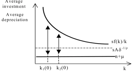
If ρ>-1, i.e., when the elasticity of substitution is high (σ>1), the growth rate of physical capital becomes,
) ( / 1 µ δ ρ − + =sA − n k k& (11) We have plotted this growth rate in Figure 1. The growth rate of k is equal to the
difference between the average depreciation line (n+µ) and the average investment line (sf(k)/k). k n+µ sAδ-1/ρ k1(0) sf(k)/k A verage investm en t A verage d epreciatio n k2(0)
Fig. 1. Growth rate of k with CES technology
In the long run, physical capital per worker and thus income per worker will grow at a positive rate even in the absence of technological progress. In the short run, provided that two economies share the same structural characteristics, income levels will approach a common value. It is possible to compute the speed of convergence (β) of income per worker around the steady state:
* log log y y dt y d β − = (12)
where y* is the steady state income per worker level. We arrive at:
+ − + − = −ρ µ δ µ β n sA n ) 1 ( (13)
The speed of convergence is a function of the savings ratio, s, and the technology parameter, A; contrary to what happens in a Solovian growth model with Cobb-Douglas technology. When the elasticity of substitution is high, i.e., ρ<0, β is decreasing in sA.
The Cobb-Douglas technology is a particular case of the CES technology corresponding to the situation where ρ tends to zero, which in turn implies that σ tends to 1.
Writing the CES technology in logs and computing its limit as ρ→0 we arrive at5:
α α −
=AK L1
Y with α=δ (14)
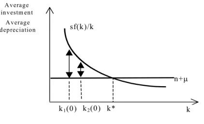
This is no more than the Cobb-Douglas technology where the input shares and the elasticity of substitution are constant. For the Cobb-Douglas specification the average product of capital approaches zero as k tends to infinity and its growth rate is equal to: ) ( ) ( ) ( 1 µ µ α − + = − + = − n k k f s n sAk k k& (15) We plotted the growth rate of k in figure 2.
k n+µ k1(0) sf(k)/k Average investm ent Average depreciation k2(0) k*
Fig. 2. Growth rate of k with Cobb-Douglas technology
5 0 0 log ) ) 1 ( log( lim 1 log log lim 0 0 = − + − = + − − → → Y A K L A ρ ρ ρ ρ ρ δ δ
. Applying L’Hôpital’s rule:
0 0
log (1 ) log
lim log log lim og log (1 ) log
((1 ) ) K K L L Y A l A K L K L ρ ρ ρ ρ ρ ρ δ δ δ δ δ δ − − − − → → + − = + = + + − + − .
In the long run physical capital per worker will stop growing in the absence of technological progress. We can also compute the speed of convergence of income per worker around its steady state and confirm that it does not depend on the savings ratio or the technology parameter.
) )( 1
( α µ
β = − n+ (16)
The parameter δ can be interpreted as a distribution parameter (see Duffy and Papageorgiou (2000, p.100)), which is equal to the capital share α in the case of the Cobb-Douglas technology. With CES technology it is harder to interpret this parameter since the capital share is a function not only of δ, but also of K, L and ρ, according to,
ρ ρ ρ δ δ δ − − − − + = L K K sk ) 1 ( (17)
Since sk∈[0,1], then δ∈[0,1]. Furthermore, ∂sk/∂δ>0, for given K, L and ρ, the
higher is δ, the higher the capital share.
3. EMPIRICAL ANALYSIS
Our sample consists of seventeen European countries: fourteen of the fifteen EU members6 and also Iceland, Norway, and Switzerland. We have annual data from 1960
to 1987 from the World Bank STARS database used by Duffy and Papageorgiou (2000). The data for GDP and the physical capital stock was converted from national currency units into constant 1987 dollars. Labour force data refers to working age population (aged 14-64). Human capital data was taken from Nehru, Swanson and Dubey (1995), the only one to our knowledge that has annual data for human capital. The human capital measure was corrected for dropouts and grade repeaters. The values for Ireland however were rather high and also decreasing so we used the Barro and Lee (2000) to get the human capital data for Ireland by polynomial interpolation.
3.1 STATIONARITY ANALYSIS OF logYIT, logYPIT, logKIT, logLIT, logHIT, and
logHLIT7 - TIME SERIES
We are going to analyse the characteristics of the six time series Yit, YPit, Kit,
Lit, Hit, and HLit in logs for each country. The series logYPit was computed using the
Hodrick-Prescott filter from the series logYit correcting for end points. Considering
potential GDP in growth studies instead of actual GDP allows us to deal with two issues: a) the influence of the cyclical behaviour of each country in the growth performance, and b) the error structure of the model is not a function of the dependent variable. We can in this way deal with the endogeneity problem that affects growth studies.
We want to determine if the series are stationary or integrated of order 1. We consider that a variable is integrated of order 1 if at least one of the ADF test -
( 1) or t n
ρ
ρ ∧
∧
− − does not allow us to reject the unit root hypothesis8. The number of
lags included in the ADF equation was determined according to an LM test to the null hypothesis of no serial correlation. We first estimate the model with trend, and, if the null hypothesis concerning its coefficient is not excluded, we estimate the model with intercept only. We present the results in table 1.
TABLE 1 – Results of the unit root tests of the series logY, logYP, logK, logL, logH and logHL.
Countries Model logY logYP logK logL logH logHL
ISL T 0 1 1 1 C 1 1 IRL T 1 1 1 C 1 1 1 PRT T 1 1 1 1 C 1 1 GRC T 1 1 1 C 1 1 1 NOR T 1 1 1 1 1 C 1 FIN T 1 1 1 C 1 1 1 DNK T 1 1 1 C 1 1 1 AUT T 1 1 C 1 1 1 1 7 Y
it – Real GDP in country i at time t; YPit – Potential real GDP in country i at time t, Kit – physical
capital stock in country i at time t t, Lit – labour force in country i at date t, Hit – Human capital in country
i at time t, HLit – human capital adjusted labour force in country i at time t. 8 We consider a 5% significance level.
Countries Model logY logYP logK logL logH logHL BEL T 1 C 1 1 1 1 1 SWE T 1 1 1 1 1 C 1 SWT T 1 1 1 1 C 1 1 NLD T 1 C 1 1 1 1 1 SPA T 1 1 1 1 C 1 1 UK T 1 1 1 1 C 1 1 IT T 1 1 1 C 1 1 1 FRA T 1 1 1 C 1 1 1 DEU T 1 1 1 1 C 1 1
Note – The countries are presented in ascending order of its average incomer per capita, 0 – stationary series and 1 – series integrated of order 1; T – model with trend; C – model with intercept and without trend.
From the results presented in table 1 we should retain that all series are integrated of order 1 since we cannot reject the null hypothesis of a unit root at the 5% level9. This kind of analysis is very important since it determines the suitable estimation
procedures but we must also test for stationarity in a panel data framework.
3.2 STATIONARITY ANALYSIS OF logY, logYL, logYHL, logYP, log, logYPHL,
logK, logKL, logKHL logL, logH, logHL, (logKL)2 and (logKHL) - PANEL DATA
We also tested our series for stationarity in a panel data framework focusing on the series used to test for Kmenta’s (1967) log linearization of the CES production function10. We will used this series later (see 3.5 and 3.6) to test the log linear CES
production function specification. We carried out this stationarity analysis using the Hadri (2000) test that considers stationarity as the null hypothesis. We estimated the model with trend (T) and without trend (WT) (see tables 2, 3 and 4).
9 With the exception of Real GDP for Iceland, which is stationary around a trend. 10 Also used by Duffy and Papageorgiou (2000)
TABLE 2 – Results from the tests for stationarity of the series logY, lnYL, logYHL,
logYP, logYPL, logYPHL
logY logYL logYHL logYP logYPL logYPH L
WT T WT T WT T WT T WT T WT T
Z 23.10 5561 22.1 3560 20.8 1272 23.32 9327 22.5 5617 21.49 3393
SL 0 0 0 0 0 0 0 0 0 0 0 0
Note SL – Significance level; z – Hadri’s statistic; WT – model without trend; T – model with trend
TABLE 3 – Results from the tests for stationarity of the series logK, logKL, logKHL,
(logk)2, (logkL)2 and (logkHL)2 .
logK logKL logKHL (logKL)2 (logKHL)2
WT T WT T WT T WT T WT T
Z 23.4 7457 22.9 5259 22.45 3595 23 5679 22.5 3831
SL 0 0 0 0 0 0 0 0 0 0
Note SL – Significance level; z – Hadri’s statistic; WT – model without trend; T – model with trend
TABLE 4 - Results from the tests for stationarity of the series logL, logH, logHL
logL logH logHL
WT T WT T WT T
Z 22.32 10122 18.6 5130 21.8 31705
SL 0 0 0 0 0 0
Note SL – Significance level; Z– Hadri’s statistic; WT – model without trend; T – model with trend
In face of these results we rejected the null hypothesis of stationarity for all the series analysed. Considering again the time series results from sections 3.1 and 3.2 it is not possible to reject the existence of a unit root for each series in each country with the exception of the series logy for Iceland (3.1). Also we reject the null hypothesis of stationarity in panel for all the series. This means that the traditional estimation procedures should not be used in this case due to the spurious regression problem. Nevertheless, in the next section we use the maximum likelihood (ML) estimation procedure to estimate the CES production function for each country. For every country we test for the presence of unit root in the residuals of each equation through an ADF test.
3.3 ESTIMATES OF THE CES PRODUCTION FUNCTION IN LOGS FOR EACH COUNTRY THROUGH ML
Following Duffy and Papageorgiou (1999), we consider the non-linear CES aggregate production function:
[
]
t it it it it A K L e Y ρ λ ε ν ρ ρ δ δ − + − − − + = 0 (1 ) (18)where A0 is the initial value (1960) of the scale effects parameter with Hicks-neutral technological progress. 0 t t A =A eλ (19)
Considering the aggregate production function in logs,
0
2 , 1
log log log (1 )
= + with (0, ) it it it it it i t t t Y A t K L N ρ ρ ν ν λ δ δ ε ρ ε ρε ν ν σ − − − = + − + − + (20)
We estimate equation (20) focusing on the estimates of ρ. If ρ<0, then σ=1/(1+ρ)>1, i.e., we reject the Cobb-Douglas specification which in turn implies that we cannot reject the endogenous growth hypothesis. The estimates were carried out considering potential GDP and either the raw labour force (L) or the human capital adjusted labour force (HL). We also tested for CR imposing v=1through an Wald test. When the hypothesis was not rejected we estimated a RLM with v=1. We imposed in our ML estimated an AR(1) error structure and we corrected the var/cov matrix for heteroscedasticity using the White procedure (see table 5).
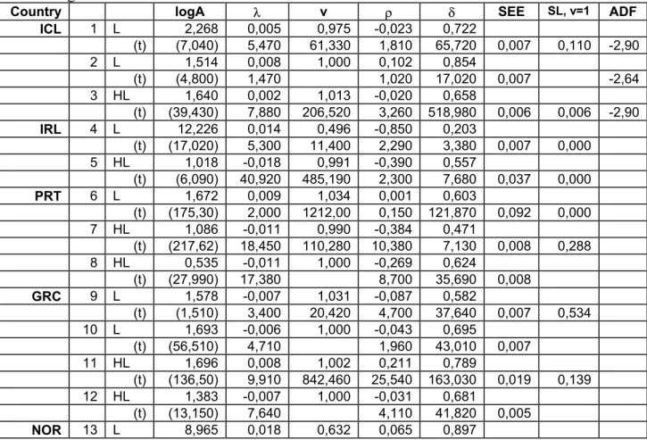
TABLE 5 – Results from the estimate of the CES production function for each country through ML
Country logA λ v ρ δ SEE SL, v=1 ADF
ICL 1 L 2,268 0,005 0,975 -0,023 0,722 (t) (7,040) 5,470 61,330 1,810 65,720 0,007 0,110 -2,90 2 L 1,514 0,008 1,000 0,102 0,854 (t) (4,800) 1,470 1,020 17,020 0,007 -2,64 3 HL 1,640 0,002 1,013 -0,020 0,658 (t) (39,430) 7,880 206,520 3,260 518,980 0,006 0,006 -2,90 IRL 4 L 12,226 0,014 0,496 -0,850 0,203 (t) (17,020) 5,300 11,400 2,290 3,380 0,007 0,000 5 HL 1,018 -0,018 0,991 -0,390 0,557 (t) (6,090) 40,920 485,190 2,300 7,680 0,037 0,000 PRT 6 L 1,672 0,009 1,034 0,001 0,603 (t) (175,30) 2,000 1212,00 0,150 121,870 0,092 0,000 7 HL 1,086 -0,011 0,990 -0,384 0,471 (t) (217,62) 18,450 110,280 10,380 7,130 0,008 0,288 8 HL 0,535 -0,011 1,000 -0,269 0,624 (t) (27,990) 17,380 8,700 35,690 0,008 GRC 9 L 1,578 -0,007 1,031 -0,087 0,582 (t) (1,510) 3,400 20,420 4,700 37,640 0,007 0,534 10 L 1,693 -0,006 1,000 -0,043 0,695 (t) (56,510) 4,710 1,960 43,010 0,007 11 HL 1,696 0,008 1,002 0,211 0,789 (t) (136,50) 9,910 842,460 25,540 163,030 0,019 0,139 12 HL 1,383 -0,007 1,000 -0,031 0,681 (t) (13,150) 7,640 4,110 41,820 0,005 NOR 13 L 8,965 0,018 0,632 0,065 0,897
Country logA λ v ρ δ SEE SL, v=1 ADF ICL 1 L 2,268 0,005 0,975 -0,023 0,722 (t) (7,040) 5,470 61,330 1,810 65,720 0,007 0,110 -2,90 2 L 1,514 0,008 1,000 0,102 0,854 (t) (4,800) 1,470 1,020 17,020 0,007 -2,64 3 HL 1,640 0,002 1,013 -0,020 0,658 (t) (39,430) 7,880 206,520 3,260 518,980 0,006 0,006 -2,90 (t) (2,500) 3,650 3,560 1,330 9,070 0,006 0,038 14 HL 10,988 0,016 0,569 -0,517 0,273 (t) (15,160) 12,270 18,130 48,390 25,920 0,006 0,000 FIN 15 L 3,055 0,012 0,958 0,092 0,784 (t) (6,940) 6,330 63,050 4,870 84,060 0,005 0,006 16 HL 1,133 0,009 1,004 -0,203 0,516 (t) (334,59) 2,230 3150,40 18,590 60,190 0,154 0,000 -5,91 DNK 17 L 2,589 0,007 1,006 0,231 0,880 (t) (30,460) 13,100 426,870 39,860 530,820 0,005 0,006 18 HL 1,795 0,004 1,026 0,271 0,849 (t) (32,900) 2,970 542,650 10,400 98,330 0,015 0,000 -2,28 AUT 19 L 1,779 -0,008 1,040 -0,064 0,589 (t) (19,220) 28,160 280,230 27,430 188,270 0,006 0,000 20 HL 2,023 -0,007 0,972 -0,035 0,706 (t) (18,550) 8,490 174,070 1,770 56,620 0,005 0,000 BEL 21 L 1,872 -0,066 1,052 -0,002 0,692 (t) (12,570) 0,420 111,760 0,050 13,060 1,191 0,000 22 HL 2,223 -0,002 0,965 -0,349 0,417 (t) (8,320) 5,810 73,170 20,130 50,380 0,009 0,007 SWE 23 L 1,232 -0,005 1,012 -0,174 0,603 (t) (225,78) 3,730 2546,20 0 101,740 590,750 0,040 0,000 24 HL 1,755 -0,003 0,986 -0,027 0,712 (t) (7,170) 3,330 103,730 1,310 49,520 0,005 0,135 25 HL 0,241 -0,003 1,000 -0,104 0,533 (t) (14,130) 3,540 5,470 303,760 0,005 SWT 26 L 2,420 -0,007 1,014 0,068 0,761 (t) (8,100) 3,610 114,490 3,390 60,630 0,006 0,120 -2,83 27 L 1,667 -0,007 1,000 0,171 0,909 (t) (24,920) 5,420 9,910 155,680 0,006 -4,54 28 HL 1,607 -0,004 0,950 0,380 0,982 (t) (49,700) 3,090 161,770 39,820 380,900 0,013 0,000 -6,18 NLD 29 L 1,306 -0,035 1,018 -0,149 0,636 (t) (291,99) 6,200 2227,10 30,310 245,290 0,244 0,000 30 HL 6,220 -0,002 0,787 -0,865 0,178 (t) (12,700) 2,330 41,870 546,90 25,240 0,003 0,000 -4,66 SPA 31 L 1,602 -0,015 1,037 -0,162 0,507 (t) (7,430) 1,870 139,300 0,950 2,820 0,017 0,000 32 HL 0,844 -0,012 0,986 -0,603 0,526 (t) (3,580) 0,490 66,380 5,450 6,660 0,078 0,365 -3,64 33 ACH 0,677 -0,014 1,000 0,063 0,872 (t) (12,270) 4,160 0,310 9,980 0,016 UK 34 L 2,456 0,006 1,050 0,170 0,759 (t) (10,840) 6,140 130,880 14,480 135,850 0,005 0,000 35 HL 4,765 0,003 0,862 0,239 0,891 (t) (13,040) 2,880 72,430 29,590 246,140 0,005 0,000 -7,49 IT 36 L 1,765 0,004 1,040 0,012 0,450 (t) (297,70) 0,320 1533,60 0,700 417,630 0,046 0,000 37 HL 1,256 -0,049 1,013 -0,094 0,660
Country logA λ v ρ δ SEE SL, v=1 ADF ICL 1 L 2,268 0,005 0,975 -0,023 0,722 (t) (7,040) 5,470 61,330 1,810 65,720 0,007 0,110 -2,90 2 L 1,514 0,008 1,000 0,102 0,854 (t) (4,800) 1,470 1,020 17,020 0,007 -2,64 3 HL 1,640 0,002 1,013 -0,020 0,658 (t) (39,430) 7,880 206,520 3,260 518,980 0,006 0,006 -2,90 (t) (9,480) 2,160 161,870 0,390 22,140 0,348 0,033 FRA 38 L 2,232 -0,004 0,982 0,053 0,807 (t) (7,680) 3,170 95,000 4,830 138,250 0,004 0,076 -3,45 39 L 1,689 -0,004 1,000 0,077 0,833 (t) (43,130) 4,130 5,800 123,240 0,004 40 HL 1,620 -0,008 0,986 -0,025 0,746 (t) (40,270) 7,850 580,330 1,660 7447,00 0,006 0,000 -2,91 DEU 41 L 1,904 -0,006 0,985 -0,071 0,701 (t) (6,050) 7,050 77,790 6,780 58,040 0,004 0,247 42 L 1,489 -0,007 1,000 -0,072 0,705 (t) (18,950) 13,150 4,620 34,710 0,004 43 HL 5,780 -0,002 0,839 -0,295 0,416 (t) (4,970) 1,360 18,770 9,710 12,720 0,004 0,000 -4,16
Note: when the unit root hypothesis is not rejected we do not present the results from the ADF test.
L – model with raw labour force, HL – model with human capital adjusted labour force. t-statistic values in brackets. SL- significance level.
Through the inspection of the results presented in table 5 we conclude that the estimated value of ρ is negative, except for Denmark, Switzerland and the United Kingdom. As for Iceland, according to equation 2 we are not able to reject the null hypothesis. However, considering equations 1 and 3 we can accept for both models that ρ is negative. Portugal has a negative estimate for ρ in the human capital adjusted model only (equations 7 and 8). We get in equation 11 a positive estimate of ρ for Greece but when we impose CRS (equation 12) ρ becomes negative. Norway and Finland present a negative estimate of ρ for the model with human capital, while Austria, Belgium, Sweden and the Netherlands present negative estimates of ρ in both models. Spain also has a negative estimate of ρ in equations 31 and 32 but not in the human capital adjusted model with CRS. Italy and France present a negative ρ in the human capital adjusted model, and finally Germany presents a negative ρ in both models.
We recall that we could not reject the null hypothesis of the presence of a unit root in the series used. According to the ADF test the only residuals that can be considered stationary are those in equations 1, 2, 3, 16, 18, 26, 27, 28, 30, 32, 35, 38, 40 et 43. This means that the conventional estimation procedures do not eliminate the
spurious regression problem. Nevertheless we can conclude that the estimated value of ρ is negative for most countries.
3.4 ESTIMATION OF THE CES PRODUCTION FUNCTION USING GMM
Unobserved country effects may cause the fact that our estimates differ. Following again Duffy and Papageorgiou (2000) we are going to estimate equation (21) that considers these effects using GMM (see also Hansen and Singleton (1982)) and sets v equal to 1. , 1 , 1 , 1 , 1 (1 ) 1 log log (1 ) it it it it i t i t i t i t Y K L Y K L ρ ρ ρ ρ δ δ λ ε ε ρ δ δ − − − − − − − − + − = − + − + − (21)
We carried out the same estimation procedure considering 3-period lags for the IV. The results of the Wald test allowed us to reject the null hypothesis of over-identified instrumental variables. The var-covar matrix was corrected for heteroscedasticity. In table 6 we present the estimation results for the sample of 17 countries and also for the group of the 4 poorest countries.
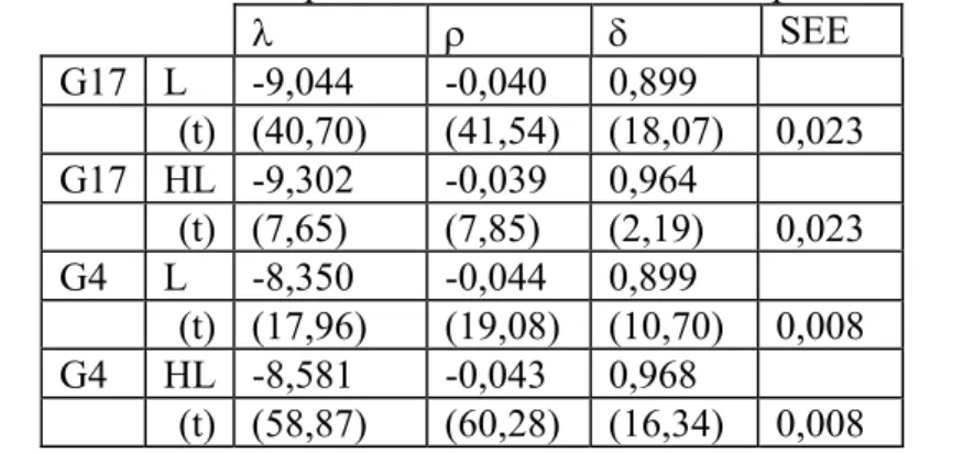
TABLE 6 – Results of the GMM panel estimation for the CES production function
λ ρ δ SEE G17 L -9,044 -0,040 0,899 (t) (40,70) (41,54) (18,07) 0,023 G17 HL -9,302 -0,039 0,964 (t) (7,65) (7,85) (2,19) 0,023 G4 L -8,350 -0,044 0,899 (t) (17,96) (19,08) (10,70) 0,008 G4 HL -8,581 -0,043 0,968 (t) (58,87) (60,28) (16,34) 0,008
Note: G17 –sample of 17 countries, G4 – sample consisting of the 4 poorest countries (Iceland, Ireland, Portugal and Greece) , SEE – standard error of the estimation. t-statistic between brackets.
The estimate of ρ is negative in both samples. δ is significant in both cases and its estimated value is theoretically acceptable although a bit too high. Our results are opposite to those of Duffy and Papageorgiou (2000, p.99) - λ is too low while δ is too high.
Finally we would like to point out that the restriction v=1 should have been tested but estimating the model without imposing the coefficient restriction would lead to computational difficulties hard to overcome.
3.5 Estimation of Kmenta’s log linearisation of the CES production function by GLS with panel data
We also estimated Kmenta’s (1967) log linearisation of the CES production which allows us to indirectly determine ρ and δ .
We now estimate equation11:
[
]
21
logyit = +α λt+β logkit+β2 logkit + εit (22)
Using the results of our estimations it is then possible to compute the values of the CES production function parameters through,
2 1 1 1 0 2 (1 ) A eα β ρ β β δ β = − − = = (25)
We can estimate equation (22) using two different methodologies: a) dynamic panel data techniques, or b) cointegration in panel data. Unfortunately using the Arellano and Bond (1991), Arellano and Bover (1995) and Doornik, Hendry, Arellano and Bond (2001) estimation procedures for dynamic panel data we obtained an estimated δ higher than one. This is the reason why we only present the results from the static panel data analysis using GLS12.
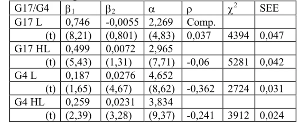
TABLE 7 – Results from the estimation of Kmenta’s log-linearisation of the CES production function through GLS
G17/G4 β1 β2 α ρ χ2 SEE G17 L 0,746 -0,0055 2,269 Comp. (t) (8,21) (0,801) (4,83) 0,037 4394 0,047 G17 HL 0,499 0,0072 2,965 (t) (5,43) (1,31) (7,71) -0,06 5281 0,042 G4 L 0,187 0,0276 4,652 (t) (1,65) (4,67) (8,62) -0,362 2724 0,031 G4 HL 0,259 0,0231 3,834 (t) (2,39) (3,28) (9,37) -0,241 3912 0,024
Note: G17 –sample of 17 countries, G4 – sample consisting of the 4 poorest countries (Iceland, Ireland, Portugal and Greece), SEE – standard error of the estimation. t-statistic between brackets. χ2 –chi-square statistic values; Comp.- ρ
was computed and not estimated.
11 Variables measured in per worker units. 12 Two stage estimate beginning with OLS.
We tested the suitability of the fixed effects specification (χ2
17 et χ24). The
results do not reject the presence of these effects. The trend coefficient is always significant. We also tested for the following error structure in all the equations:
it it 1− it
ε = ϕ⋅ε + υ . This seems a suitable specification to test for the stationarity of the error term.
TABLEAU 8 – Results from the estimation of the residuals for equations G17L, G17HL, G4L and G4HL Residuals from equation: HT tρ ρ_ stat G17 L -0,042 661,1 0,06 (SL) (0,48) (0.0) (0,48) G17 HL -0,042 680,4 0,06 (SL) (0,48) (0.0) (0,48) G4 L 0,022 639,7 0,03 (SL) (0,49) (0,0) (0,49) G4 HL 0,02 735,5 0,03 (SL) (0,49) (0,0) (0,49)
Note – HT-Harris&Tzavalis-statistic values, SL – significance level, tρ and ρ_ stat- Levis&Lin-statistic values. The values of the HT-statistic allow us to accept the existence of a unit root. The Levis&Lin (1992) – statistic on the other hand contradicts this result. The first test leads us to reject the unit root hypothesis while the second test points to the presence of a unit root. This means that we cannot dismiss the spurious regression problem in all four equations. Nevertheless this is a quite important result since most empirical growth studies do not carry out a stationarity analysis of the series used within a panel data framework13 thus its conclusions may not apply due to the spurious regression problem.
The results presented in table 7 state that for equation G17L it is not possible to reject the null hypothesis for the estimate of β2, while in equation G17HL we can only
accept this hypothesis for a 19% confidence level. This is not a very encouraging result. We still get a negative estimate of ρ in equation G17HL and for both equations in G4.
3.6 Estimation of Kmenta’s log linearisation of the CES production function by panel cointegration methods
We now estimate Kmenta’s (1967) log linearisation of the CES production using cointegration techniques for panel data. The model estimated does not include an intercept,
[
]
21
logyit =λ βt+ logkit+β2 logkit + εit (22.a)
First, we used Kao (99) tests and three Pedroni (99) test that test for the null hypothesis of no cointegration. In the former we used a one-period lag. The V-statistic is computed through the within estimation procedure and the ρ_stat is computed through the between estimation procedure.
TABLE 9 - COINTEGRATION TESTS BASED ON KAO’S AND PEDRONI’S METHODS APPLIED TO EQ. (22)
G17L G17HL G4L G4Hl Kao99 DF ρ test -0,49 (0,31) -0,48 (0,31) -1,82 (0,03) -0,70 (0,24) Kao99 DF tρ test -0,93 (0,18) -0,71 (0,24) -1,10 (0,13) -0,12 (0,45) Kao99ADF(lag=1) -1,86 (0,03) -1,85 (0,03) -1,76 (0,04) -2,02 (0,02) Pedroni99 t_stat -477 (0,000) -477 (0,000) -100,84 (0,00) -107,54 (0,00) Pedroni99 V_stat -3,49 (0,000) -3,54 (0,000) -1,47 (0,07) -1,68 (0,05) Pedroni99 ρ _stat 6,12 (0,000) 6,12 (0,000) 2,76 (0,00) 3,02 (0,00)
Note – The significance level of each statistic is presented in brackets.
In almost all cases the first two Kao’s tests do not allow us to reject the null hypothesis of no cointegration, while all other tests do allow us to reject this hypothesis. Based on these results we proceed to the estimation of the cointegration relations for the four models.
We used the Kao and Chiang (2000) estimation procedure imposing an heterogeneous matrix of var-covar for the sample of 17 countries and an homogeneous matrix of var-covar for the sample of four countries14. We used a one-period lag and a
one-period lead.
TABLE - 10 Results from the estimation of Kmenta’s log-linearisation of the CES production function using panel cointegration techniques
λ β (=δ)1 β 2 ρ R2 G17L 0,0806 0,0580 0,0372 (t) (65193) (7,97) (5,73) -1,36 0,57 G17HL 0,0144 0,0338 0,0361 (t) (18387) (1,42) (3,34) -2,2 0,57
G4 HL 0,2590 0,0533
(t) 2,43 3,34 -0,55 0,98
For the sample of the 4 poorest countries it was never possible to reject the null hypothesis of no trend. In the models with L δ is negative.
With the exception of G4HL, the estimated values of β (1 δ) are very low and ρ is negative. Nevertheless the estimated ρ with human capital is quite lower than in the model without human capital.
CONCLUSION
The main goal of this paper was to distinguish between the potential sources of growth and convergence for the Portuguese economy within Europe. We followed the methodology of Duffy and Papageorgiu (2000) developing a little further their econometric analysis. It is important to determine whether the most suitable specification of the aggregate production function is a CES technology or a Cobb-Douglas technology since this distinction has important implications for growth. For instance, if the elasticity of substitution between inputs is greater than one (σ>1) then the economy is characterised by endogenous growth (see Jones and Manuelli (1990), Rebelo (1991)). If (σ<1) on the other hand, Azariadis (1993, 1996, 2001) shows that the economy can converge to different steady-states depending on its initial conditions.
From our econometric analysis we concluded that ρ<0, i.e., the CES technology is the one that best describes the technology used in each of the seventeen countries in our sample. This result supports that of Duffy and Papageorgiou (2000) and implies the development of growth models without balanced growth.
As far as convergence is concerned the implications of our analysis are derived from the results in tables 6 and 7 (estimated values of ρ, δ and β1) through the analysis
of the sample of 17 countries and the sample of the 4 poorest countries.
According to the results in table 6 we get a higher value of ρ for the G4 sample whatever the model consider. This result means that there will not be convergence between the economies in our sample since the higher ρ is (in absolute value) the lower the difference between the terms sAδ−1/ρ and n+µ for the G4 in comparison with the
growth rate of the G17 in the transition period. This conclusion is further reinforced by the fact that in the model with labour force the estimated value of δ is the same for both samples15 - everything else equal, economies with a higher value of δ, will have a
higher income per capita growth rate. In the model with human capital adjusted labour force, the estimated value of δ is higher for the G4 but only 0.004 higher than for the G17, which is a very small difference. If we focus on the results for the first model then we conclude that there will be no convergence between the G4 and the G17. If we focus on the results for the human capital adjusted model although there is convergence it proceeds at a very low speed. Both results are not encouraging for the G4 economies.
According to table 7, the estimated values of ρ and δ in the human capital adjusted model point to the rejection of the convergence hypothesis between the G4 and the G17- the estimated value of ρ is higher for the G4 while the estimated value of δ is lower for this sample. Again convergence proceeds at a very slow pace.
The main contributions of our empirical analysis are the following. First, by considering the potential value of GDP and not its effective value we are able to overcome the endogeneity problem. Second, the conclusions of the conventional empirical growth studies are not valid in the presence of non-stationary series. This is why we tested all the series for stationarity both in a time series and in a panel data framework. In all the estimations carried out (ML, GMM, static panel) we devoted a considerable amount of time to the stationarity analysis of the series used and of the residuals of the estimated equations. We also tested for cointegration relationships. Despite this careful analysis some of the estimated coefficients present values that are not easily justified. This is a possibility for future research since it calls for the analysis of non-linear cointegration relations within a panel data framework.
15 Although the estimated value of δ is a little too high, nevertheless it is significant and supported by the
BIBLIOGRAPHY
[1] Arellano, M. and Bond, S. (1991), “Some tests of specification for panel data : Monte Carlo evidence and an application to employment equations”, Review of Economic Studies, 58, 277-97.
[2] Arellano, M. and Bover, O. (1995), “Another look at the instrumental variables estimation of error-components models”, Journal of Econometrics, 68, 29-51.
[3] Azariadis, Costas (1993). Intertemporal Macroeconomics. Oxford. Blackwell Publishers. February.
[4] Azariadis, Costas (1996), "The Economics of Poverty Traps, Part One : Complete Markets", Journal of Economic Growth, pp. 449-486.
[5] Azariadis, Costas (2001), "The Theory of Poverty Traps: What Have we Learned?", mimeo, July, http://www.econ.ucla.edu/azariadi/#Publications.
[6] Barro, R. (1991), “Economic growth in a cross section of countries”, Quarterly Journal of Economics, Vol. 106(2), May, pp. 407-443.
[7] Barro, R. and Sala-I-Martin, X. (1995), Economic Growth, McGraw-Hill International Editions.
[8] Benhabib, J. and Spiegel, M. (1994), “The role of human capital in economic development: evidence from aggregate cross-country data”, Journal of Monetary Economics, Vol. 34, pp. 143-173.
[9] Chiang, M-H and Kao, C. (2002), “Nonstationary panel time series using NPT 1.3 – A user guide”.
[10] Doornik, J., D. Hendry, M. Arellano. and S. Bond, (2001), “Panel data models (DPD)”, dans Doornik, J. and Hendry, D. Econometric modelling using PcGive, Volume III, pp. 61-98, Timberlake, London.
[11] Duarte, A. and Simões, M. (2000), “Le rôle de l’investissement dans l’éducation (total et par genre) dans la croissance. Une étude appliquée à l’échantillon de pays riverains de la Méditerranée”, 4EMES RENCONTRES EURO-MEDITERRANEENNES: "Inégalités et pauvreté dans les pays riverains de la Méditerranée", Nice, September.
[12] Duarte, A. and Simões, M. (2001a), “Le rôle de l’investissement dans l’éducation sur la croissance selon différentes spécifications du capital humain. Une étude appliquée à l’échantillon de pays riverains de la Méditerranée, 5EMES RENCONTRES EURO-MEDITERRANEENNES: “Systèmes Éducatifs, emploi et migrations dans l’espace euro-méditerranéen”, Nice, France, September.
[13] Duarte, A. and Simões, M. (2001b), “Principais factores de crescimento da economia portuguesa no espaço europeu”, Comunicação apresentada na IVª Conferência – Como está a Economia Portuguesa?, ISEG, Lisbon, Portugal, May. [14] Duarte, A. and Simões, M. (2001c), “A Especificação da Função de Produção
Macro-Económica em Estudos de Crescimento Económico, uma análise de dados de painel aplicada a um grupo de países europeus”, IV ENCONTRO DE ECONOMISTAS DE LÍNGUA PORTUGUESA, Évora, Portugal, October.
[15] Duffy, J. and Papageorgiou, C. (1999), “A cross-country empirical investigation of the aggregate production function specification”, Journal of Economic Growth, 5(1), pp. 87-120, March.
[16] Hadri, K. (2000), “Testing for stationarity in heterogeneous panel data”, Econometrics Journal, 3 (2). 148-61.
[17] Hansen. L.P and Singleton, K.J. (1982), “Generalised instrumental variables estimation of non-linear rational expectations models”, Econometrica, 50, 1269-1286.
[18] Harris, R. and Tzavalis, E. (1999), “Inference for unit roots in dynamic panels where the time dimension is fixed”, Journal of Econometrics, 91, 201-26.
[19] Islam, N. (1995), “Growth empirics: a panel data approach”, Quarterly Journal of Economics, vol. 110(1195), November, pp. 1127-1170.
[20] Jones, L.E. and Manuelli, R.E. (1990), “A convex model of equilibrium growth: theory and policy implications”, Journal of Political Economy, vol. 98, pp. 1008-1038.
[21] Kao, C. (1999), “Spurious regression and residual-based tests for cointegration in panel data”, Journal of Econometrics, 90, 1-44.
[22] Kao, C. and Chiang, M. (2000), “On the estimation and inference of a cointegrated regression in panel data”, Advances in Econometrics, 15, 179-222. [23] Levin, A. and Lin, C-F. (1992), “Unit root tests in panel data: asymptotic and
[24] Lucas, R. E. (1988), “On the mechanics of economic development”, Journal of Monetary Economics, vol. 22, pp. 3-42.
[25] Mankiw, N.; Romer D. and Weil, D. (1992), “A contribution to the empirics of economic growth”, Quarterly Journal of Economics, vol. 107, pp. 407-437.
[26] Pedroni, P. (1999), “Critical Values for Cointegration Tests in Heterogeneous Panels with Multiple Regressors”, Oxford Bulletin of Economics and Statistics, 61, 653-78.
[27] Rebelo, S. (1991), “Long-run policy analysis and long-run growth”, Journal of Political Economy, vol. 99, pp. 500-521.
[28] Romer, P. (1986), “Increasing returns and long-run growth”, Journal of Political Economy, vol. 94, pp. 1002-1037.
[29] Simões, Marta (1999), Convergência de acordo com a Teoria do Crescimento: estudo de algumas hipóteses com aplicação à União Europeia, Dissertação de Mestrado em Economia, Faculdade de Economia da Universidade de Coimbra, pp. 330.
[30] Simões, Marta (2000), “La Convergence Réelle Selon la Théorie de la Croissance: Quelles Explications Pour l'Union Européenne?”, Économie Appliquée, Tome LIII, nº4, December.
[31] Solow, R. (1956), “A contribution to the theory of economic growth”, Review of Economics and Statistics, vol. 39, pp. 312-320.
[32] Solow, R. (1957), “Technical change and the aggregate production function”, Quarterly Journal of Economics, vol. 70(1), pp. 65-94.