Cost Behavior - an empirical Investigation for Euro Area Countries

I

Cost Behaviour – an empirical investigation for Euro Area Countries

Diana Filipa Cruz Costa

Dissertation

Master in Finance and Taxation

Supervised by

Prof. Doctor Samuel Pereira (a) Prof. Doctor Elísio Brandão (a)

(a) University of Porto, School of Economics and Management

I

Biographical note

Diana Filipa Cruz Costa is a Portuguese national born on 25th of January of 1995 in Vila Nova de Famalicão. She joined School of Economics and Management, University of Porto (FEP) in 2013 and graduated in Economics in 2016, with a final grade of 16. In the same year she enrolled in Master of Finance and Taxation in FEP, to which she is now a candidate to obtain the master’s degree.

She completed high school in 2013 at Escola Secundária da Trofa with a final average of 19 values. There she was member of the Students' Association.

On a professional level, the only experience she had was an internship at a prestigious consulting firm with a worldwide presence. This internship took place within the scope of this master's degree, between October 2017 and March 2018.

II

Acknowledgements

I would like to thank my supervisors (PhD Professor Samuel Pereira and PhD Professor Elísio Brandão) for all guidance they gave me, from the beginning, starting with the selection of the theme of my dissertation until the end, with the realization of it. Certainly, without their assistance it would be almost impossible to achieve this work. Additionally, I would also like to thank a lot PhD Professor Francisco Vitorino, because although he was not my supervisor, he was always available to help me in econometric issues.

To all my colleagues in Master and to all the professors I had during my academic life, thank you very much for your contribution to the person I am today.

Last, but not least, I would like to thank all the support that my family and friends, specially Francisco Fernandes, gave me during this journey. It was an amazing period of my life, precisely because I managed to overcome myself and achieve the goals that I set myself, but without them it would never be possible.

III

Abstract

Costs are an important component for businesses as they affect the results and hence the firm position. Therefore, to understand how they vary with changes in output and what factors influence them is fundamental, not only for managers, but for all agents related to organizations.

The traditional theory predicts the existence of two types of costs, the variables and the fixed ones. However, an alternative hypothesis has emerged that accounts for an empirical phenomenon, the "cost stickiness", and later the "anti-stickiness", in which the behaviour of costs is based on discretionary management decisions, under different circumstances.

In this paper, we show that the operating costs of Euro Area companies are sticky, since in the face of a positive change in sales costs increase more than decrease when sales fall by the same amount. In addition, we have documented that this phenomenon is reinforced in countries where labour law is more rigid and those whose intervention by the Troika has been necessary, because these two aspects increase the adjustment costs.

Keywords: cost behaviour, stickiness, anti-stickiness, deliberate resource commitment, adjustment costs.

IV

Resumo

Os custos são uma importante componente para as empresas, uma vez que afetam os seus resultados e, consequentemente, a sua posição. Por isso, perceber como variam face a alterações do output e quais os fatores que os influenciam é fundamental, não só para os gestores, mas para todos os agentes relacionados com as organizações.

A teoria tradicional prevê a existência de dois tipos de custos, os variáveis e os fixos. No entanto, tem surgido uma hipótese alternativa, que dá conta de um fenómeno empírico, o “cost stickiness”, e posteriormente o “anti-stickiness”, na qual o comportamento dos custos é baseado nas decisões discricionárias de gestão, perante diferentes circunstâncias.

Neste trabalho, mostramos que os custos operacionais das empresas da Zona Euro são “sticky”, uma vez que perante uma variação positiva das vendas os custos aumentam mais do que diminuem quando as vendas baixam no mesmo montante. Adicionalmente, documentamos que este fenómeno é reforçado nos países em que a lei laboral é mais rígida e naqueles cuja intervenção da Troika foi necessária, pelo facto destes dois aspetos aumentarem os custos de ajustamento.

Palavras-Chave: comportamento dos custos, “stickiness”, “anti-stickiness”, escolhas deliberadas de gestão, custos de ajustamento.

Index of Content

2.1. Theories and Explanations for Sticky Costs... 4

2.2. Employment Protection Legislation (EPL) ... 9

2.3. The crisis affecting the Euro Area and the intervention of Troika...12

3. RESEARCH METHODOLOGY ...15 3.1. Variables ...15 3.2. Sample ...18 3.3. Empirical Models ...19 4. EMPIRICAL RESULTS ...23 4.1. Univariate Results ...23 4.2. Multivariate analysis ...32

5. ROBUSTNESS AND ADDITIONAL TESTS ...35

6. CONCLUSION...40

REFERENCES ...42

Index of tables

Table 1: Summary Statistics ...24

Table 2: Descriptive Statistics per Variable ...25

Table 2 Panel A AssetInt defined as ln((Total Asset)/(Sales Revenue)) ...25

Table 2 Panel B: ∆lnOPC defined as the first difference of the logarithm of operational costs...26

Table 2 Panel C: ∆lnSALES defined as the first difference of the logarithm of sales revenue ...27

Table 2 Panel D: GDPGrowth defined as the annual percentage growth rate of GDP at market prices based on constant local currency, where aggregates are based on constant 2010 U.S. dollars28 Table 2 Panel E: EPL defined as the mean of TempEPL and RegEPL, range from zero to six ...29

Table 2 Panel F: TempEPL is an index of employment protection legislation for temporary employees, ranges from zero to six ...30

Table 2 Panel G: RegEPL is an index of employment protection legislation for regular employees, ranges from zero to six ...30

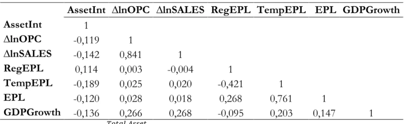
Table 3 Pearson’s Correlation...31

Table 4 Estimates of the relation between EPL, Troika and Stickiness ...34

Table 5 Robustness Tests...36

Table 6 Estimates after controlling for manager optimism and pessimism...38

Table 7 Panel A EPL for regular employees...47

Table 7 Panel B: EPL for temporary employment...49

1

1. INTRODUCTION

Understanding cost behaviour is one of the most important issues in cost accounting. This investigation is not only from a theoretical stand point, but also the practical implications for all entities, especially for companies, since their purpose is to maximize their resources to maximize their profits. Obviously, in pursuit of the main goal of companies, costs should be minimized and accounting researchers, as well as practitioners, acknowledge the importance of a firm´s cost structure to firm performance. Thus, this study is part of a recently emerging stream of research aiming to expand our understanding of cost behaviour and point out which factors are vital to explain that behaviour, whether exogenous or endogenous to the company itself.

Traditional cost behaviour models in the accounting literature distinguish between fixed and variable costs with respect to changes in the level of activity. In fact, a fundamental premise of cost accounting is that there is a symmetric relationship between variations in activity and in costs. So, a 1% increase in activity results in an increase in costs by a certain amount, as well as, a 1% decrease in activity level results in a decrease in costs by the same amount.

Recent research documents the empirical phenomenon of “sticky costs”1_{, which is} inconsistent with the traditional model of fixed and variable costs, because these costs neither behave like fixed or variable costs. However, we cannot say that the traditional theory is totally wrong or must be disbelieved. But, underlying the traditional cost behaviour model are several assumptions which, apart from simplifying the real world, distance the model from the way costs behave. So, it is acceptable that empirically we find a different cost behaviour.

1 _{Formally, costs are “sticky” if they respond less to decreases in activity than they raise for an equivalent activity}

2 In fact, these recent studies have documented strong evidence of asymmetric cost behaviour and attributes it to a theory of deliberate managerial decisions in presence of adjustment costs (Anderson et al, 2003, hereafter, ABJ). These deliberate decisions have not been associated with manipulation or other reprehensible acts in the literature related to subject, but an optimal choice to maximize resources.

Recent literature on dynamic factor demand in economics have modelled formally these decisions (e.g., Bentolila and Bertola (1990), Hamermesh and Pfann (1996), Dixit, (1997),

Goux et al. (2001)). These studies explicitly model the dynamic optimization problem faced by companies, in the presence of adjustment costs and having a future horizon and show that the optimal resource commitment decisions are generally asymmetric. Therefore, this derives the cost accounting notion of cost stickiness as a direct consequence of optimal decisions with adjustment costs. Thus, insofar as managers recognise the trade-off associated with the adjustment costs, their choices are expected to introduce a more complex dynamic in cost behaviour, resulting in cost stickiness patterns. Also, considering this potential source of asymmetry in cost behaviour, and thus, in variation of earnings, it has also been shown to be informative in forecasting earnings and understanding earnings management in accounting research (Banker and Chen (2006)).

The economic theory of optimal decisions with adjustment costs, described above, provides a theoretically sound potential explanation for the widely documented empirical patterns of cost stickiness, however it is not the only plausible one. For example, expectations of managers about future activity level can also have a strong impact in cost behaviour. Banker et al. (2014) noted that the resource expansion associated with activity increases is subject to managerial discretion and argued that this discretion can lead to anti-stickiness2

when managers are pessimistic about the future. Another possible explanation is that stickiness may also arise due to manager’s empire-building3 _behaviour.

2 _{The term “anti-stickiness” was coined for the first time by Weiss (2010). However, Weiss just showed that costs}

could be “anti-sticky” if they decrease more when sales fall than they increase when sales rise equally, but he didn´t establish when they are likely to be anti-sticky. Banker et al. (2014), contributed to answer this question.

3 Our focus will be testing the central implication of the economic theory of optimal decisions with adjustment costs. If cost stickiness reflects deliberate resource commitment decisions by managers who face adjustment costs, then the degree of stickiness must be like the magnitude of these costs. However, it is not easy to identify a reliable proxy for adjustment costs in general. Therefore, we will use indexes of employment protection legislation (EPL), which are compiled and reported by OECD for most of developed countries as reliable proxies for adjustment cost associated with labour. A stricter EPL reflects greater adjustment costs for labour, and the economic theory of sticky costs predicts that firms in a country with stricter EPL provisions will exhibit greater cost stickiness, which lead us to predict a positive relation between country-level EPL strictness and firm-level cost stickiness.

In this respect, and to the best of our knowledge, it is the first time that cost behaviour will be dealt with in the scope of this Master. So, this paper contributes to the literature in three different ways. First, using Banker et al. (2013), as the basis of our work, we replicate the models using data for a sample of manufacturing sector firms from 15 Euro Area4 _{countries, which allow us to expand their study. Also, the vast literature on the subject,}

usually studies cost behaviour for American firms. Our sample of Euro Area countries and the period that we purpose to study constitutes an innovation. Finally, the introduction of macroeconomic variables related to the countries under study is also a contribution. The understanding of cost behaviour expands, insofar as it is studied whether this behaviour is inherent to the characteristics of the companies, or if it is also affected by the conjuncture of each country, namely the intervention of Troika5_.

This paper is organised as follows. Section 2 is a brief review of literature and describes different theories of costs behaviour; Section 3 describes the research methodology; Section 4 the empirical results and Section 5 presents some robustness tests. The conclusion is presented in Section 6.

4 _{Initially, we collected information from all countries in the Euro Area (19). However, after processing the}

data, we realized that there was not enough information needed to estimate the models in Cyprus, Ireland, Lithuania and Malta. Therefore, the final sample has data from 15 countries.

5 _{Currently, Troika is referred as a decision group formed by the European Commission (EC), the European}

4

2. LITERATURE REVIEW

2.1. Theories and Explanations for Sticky Costs

The traditional view of cost behaviour distinguishes between fixed and variable costs with respect to changes in level of activity. Fixed costs are assumed to be independent of the level of activity, whereas variable costs are anticipated to change linearly to fluctuations in the level of activity, implying that the magnitude of a change in costs depends only on the extend of a change in the level of activity, not on the direction of the change (Noreen (1991)). However, it might be not totally right.

Cooper and Kaplan (1998) and Noreen and Soderstrom (1997), were the first authors to detect that, in fact, not all costs could be classified as fixed or variable costs. In their studies, they concluded that some of the costs under analysis increased more when the volume of activity increased than diminished with decreases in activity. Nevertheless, ABJ suggest that selling, general and administrative costs respond less to downward changes in activity than upward changes, a phenomenon they refer to as “sticky costs”. On average, costs increase 0,55% per 1% increase in sales, but decrease only 0,35% per 1% decrease in revenue in their sample. According to ABJ, the prevalence of these costs is consistent with the cost behaviour model in which managers adjust resources in a deliberate way in response to changes in volume and in the presence of adjustment costs1_{. For the first time a model distinguishes}

within costs that change in the face of changes in the volume of activity, those that change in a "mechanical" way from those that depend on the discretionary choices of the managers. Additionally, Subramaniam and Weidenmier (2016) confirm and extend this evidence for costs-of-goods expense.

1_{Briefly, we can say that the adjustment costs are the costs of unexpectedly changing the level of output of a}

firm, regardless of whether it is an increase or decrease thereof. For example, it may be desirable for a firm to cut down on its output but, doing so will create adjustment costs such as redundancy payments and lower staff morale. On reflection of its adjustment costs, it could be more desirable to keep producing at a sub-optimum level. Similarly, a rapid expansion of output may create problems such as difficulties in negotiating a bigger place to rent and difficulties in hiring more workers. However, this last situation demands that the resources increase, otherwise the output will not be able to increase. Then, as managers recognise the trade-offs that arise because of the adjustment costs, they will reduce resources to a lesser extent when the activity shrinks than they expand when the activity increases, causing cost stickiness.

5 There are many key factors that affect the way managers decide. For example, when future demand is uncertain, and the firm incurs in adjustment costs if it chooses to reduce or restructure its resources, managers tend to postpone these reductions until they are more certain of the effective fall in demand. It suggests that the stickiness of costs is temporary, because somewhere in the future will be reversed or made effective. So, the stickiness observed over a period may be reversed in the following period and that this feature may be less pronounced when the observation period is longer. In periods of decline in economic activity and consequent fall in sales, managers must decide whether to keep the same resources and support the operational costs of having unused capacity or support the adjustment costs related to the cut in resources. This decision will depend on the likelihood that sales will continue to fall or not. Thus, the stickiness will be stronger when the expectations of managers about the steady drop in demand are low or when the adjustment costs are greater. ABJ argue that managers hesitate to eliminate slack resources when they expect a sales drop to be temporary, causing cost stickiness when activity level decrease. However, when it is intended to increase output, it is inevitable to increase resources, since without this it is impossible to increase the level of activity of the firm.

In addition to demand uncertainty, financial risk is another factor that will likely influence manager’s decisions. Financial risk can be defined as the potential future inability of the company to honour its financial commitments and has adverse direct and indirect effects for the company. Direct consequences are intuitively identified, since if the company fails to make a financial commitment, its capital costs increase and the probability of having legal problems is higher too. Moreover, after having identified the direct consequences, Altman and Hotchkiss (2006), proved that indirect consequences can be quite significant and are unobservable opportunity costs like loss of stakeholders. Naturally, companies with an already high level of risk tend to prefer a cost structure that fits the circumstances more quickly. So, managers of these firms are more likely to take actions that increase cost elasticity to reduce additional risk, otherwise with inelastic cost structures the vulnerability to demand shocks is higher.

6 These two factors were extensively studied by Holzhacker et al. (2015), to obtain information on the mechanisms used by companies in response to these two factors. They believe that, in response to the two risk drivers, managers change their resource decisions, to increase their elasticity. In a firm with a less elastic cost structure, the decrease in demand will have a more negative impact on profit than on a company with a more elastic structure, because the same decrease in quantity will decrease a lower proportion of costs.Therefore, as demand uncertainty and financial risk increase, managers will be more likely to explore mechanisms to increase the elasticity of firm´s cost structure. In this regard, managers can take three actions, namely outsourcing, leasing or rental of equipment and restructuring of work contracts to increase the proportion of flexible ones.

Banker et al. (2014), improved the theory of sticky costs and developed empirical models. Prior research has shown that the stickiness of costs is pervasive across different cost categories and different datasets. However, these authors show that ABJ's intuition gives rise to a more complex asymmetry pattern that goes beyond their predictions and combines two processes: stickiness when there is a previous increase in sales and anti-stickiness in the case of a prior reduction of sales. They have justified these forecasts, firstly because, after a prior increase (decrease) in sales, managers' expectations for future sales are more optimistic (pessimistic), since sales changes are positively correlated over time, and behaviour economic studies suggest managers extrapolate past trends. Optimism increase managers' willingness to acquire additional resources when sales increase and to retain some unused ones when sales decrease. One the other hand, pessimism has the opposite effect. Below, they believe that managers retained significant slack resources only if sales decreased in a prior period. When sales increase, the amount of slack carried over into the current period is weak or non-existent. These two effects lead to cost stickiness in the current period only in the case of a prior sales increase, and they generate the opposite predictions of anti-stickiness following a prior sales decrease. In accordance with this finding, it was noticed that the slack resources provoke asymmetry in the behaviour of costs which is determined by the direction of the variation of the sales in the previous period. Overall, the results support ABJ's fundamental view that asymmetric costs behaviour reflects deliberate decisions of managers on a "forward-looking"2_.

2 _{This term means that managers make their decisions having as horizon the future. Basically, they make}

7 On the other hand, changes in sales may reflect changes in short-term market conditions or longer-term changes in demand for products or services. Therefore, when managers face a decrease in sales, they do not react immediately, in order to perceive the source of the change and then react accordingly. This "delay" causes cost stickiness, as the unused resources are maintained during the period between the volume reduction and the adjustment decision. Another important aspect is that costs become less sticky as revenue declines over several periods, as the expectations of the decision maker are aligned with the sales situation. If sales are constantly declining, managers will inevitably have to dispose of resources, incurring the costs of adjustment.

Prior research of sticky costs has relied on informal arguments about the trade-off that arise with adjustment costs. However, the literature of dynamic factor demand in economics has explored these trade-offs more deeply. In this dynamic context, the optimal level of resources corresponds to the amount at which the marginal adjustment costs incurred per unit of resource in the current period equals the present value of expected net cash flows generated by the marginal resource unit over its service life. When deciding how much to reduce resources when activity levels fall, managers weigh the benefits of more efficient operations against the adjustment costs they must incur. Consequently, this trade-off often causes deliberate retention of some resources that will not be used to avoid incurring adjustment costs. In addition, managers have much less discretion over the acquisition of the necessary resources when the activity increases, since even if they intend not to incur adjustment costs, this will not happen, because without resources, companies are not able to respond to increases of activity. In this way, the asymmetry provoked by managers' choices is caused by optimization decisions.

8 Despite the importance of adjustment costs in this new theory of cost behaviour, there are also other reasons that explain the sticky behaviour of costs. For example, the character of the manager may have an impact on the behaviour of costs. Authors like Anderson et al. (2003) and Chen et al. (2012), report that more empire-building managers are more reluctant to cut resources even in the presence of declining sales, thereby increasing the stickiness of some costs. In addition, when sales increase they are very likely to immediately increase the company's resources. So, if managers engage in empire-building, it can generate cost stickiness, even in the absence of adjustment costs. Additionally, Banker et al. (2014) noted that the managers' expectations about the future activity also condition the behaviour of costs, provoking stickiness. Although behavioural factors of managers do not determine the overall structure of behaviour of asymmetric costs, they accentuate or diminish their magnitude. The stickiness can also be conditioned by the existing capacity. Balakrishnan et al. (2004) have found, for example, that an organization that operates to the maximum of its capacity when confronted with a reduction in activity responds less than if it encounters an increase in activity.

Despite all explanations for cost behaviour, we believe the theory of optimal resource commitment decisions with adjustment costs provide a theoretically sound explanation for the widely documented empirical findings of costs stickiness. Moreover, according to this theory, these discretionary choices reflect a behaviour desired by the managers, who do optimal choices that increases the value of the company. The same does not happen with other possible explanations, for example with empire building theory. It is assumed that the choices of the managers may not be optimal and be harmful to the proper company, becoming a waste that withdraw value from the company.

9 2.2. Employment Protection Legislation (EPL)

As stated above, the adjustment costs play a central role in the new theory of cost behaviour. However, as the adjustment costs are implicit costs rather than explicit monetary costs expressed in accounting system (Hamermesh and Pfann, (1996)), it is not possible to measure this directly and it is not easy to obtain a proxy for these, too. For this reason, a few works have been able to study this relation. They use firm-level proxies specifically for labour factor, such as employee intensity or assets. For exemple, the first authors that document pervasive asymmetries in cost behaviour, ABJ, used both proxies. In addition, prior research used the rigidity of the labour market as proxy of the adjustment costs, a country-level proxy. We exploit these country-level proxies, but we also control for firm-level determinants of cost stickiness, following prior literature. In fact, EPL has been widely used, and has been shown to be reliable, in prior economics research (e.g., Long and Siebert (1983); Lazear (1990); Pissarides (1999); Blanchard and Portugal (2001)). According to Banker et al. (2013), the major advantage of EPL is that they are exogenous with respect to managers' decisions, so it cannot be manipulated or changed according to the will of the managers.

Historically, the first cases of statutory employment protection date back to the early twentieth century. However, the process of increasingly regulating firing and hiring, since free labour market seems to be inefficient, is a recent system that became to be stable at the 1900s. By contrast, since the global financial crisis in 2008, and according to OECD (2013), there is a clear trend of deregulation of employment protection. Obviously, this tendency is not observed in every OECD countries and they have different levels of employment protection. But, in one-third of them undertook some relaxation of regulations on either individual or collective dismissals, thereby reducing the gap in the stringency affecting temporary and permanent contracts. Interestingly, policy action was more intense in OECD countries that had most stringent legislation before the onset of the crisis, in order to liberalize the labour market. Despite this flexibility, particularly in terms of severance payments and fixed-term contracts, EPL still translates into high costs for companies when they decide to lay off.

10 In this sense, the provisions of the Employment Protection Legislation, such as the rigidity indexes of labour laws, are explored to see if the costs are in fact sticky or not. The asymmetry envisaged by the sticky cost theory might be due to deliberate decisions made by managers facing adjustment costs (such as costs of hiring and firing staff, including severance payments to dismissed workers or search and training costs when new employees are hired, or disposal losses on equipment). The manager's optimal decisions are made by analysing the trade-off between the adjustment costs associated with the hiring or firing of a marginal worker and the net present value of the cash flows (NPV) that this worker must generate during the time he remains in the company. When the activity increases, managers hire additional workers if the marginal worker's NPV exceeds the cost of hiring. On the other hand, when activity decreases, managers will lay off workers, provided that the marginal worker's NPV is negative and large enough (in absolute value) to exceed the cost of redundancy.

The results of Banker et al. (2013), show that the relationship between the stickiness of costs and the rigidity of the EPL in the data is consistent with the theory that the stickiness of costs reflects the deliberate decisions of managers. In this way, it was found that a company operating in a country with more stringent EPL (i.e., higher adjustment costs to reduce labour) will exhibit more cost stickiness, i.e. more asymmetry in cost response to changes in sales. In addition, Caballero (2013) showed that the rigidity of the EPL reduces the ability of companies to adjust to shocks, which corroborates the idea that greater rigidity of the labour law increases the costs of adjustment of the companies, consequently causing greater stickiness of the companies’ costs.

It should be noted that there is a vast literature devoted to examining the various aspects of EPL, as well as other characteristics of the labour market (e.g., Hopenhayn and Rogerson (1993); Mortensen and Pissarides (1999); Heckman et al. (2000); Botero et al. (2004)). They document that EPL is the main source of firing costs and that it has important effects on various macroeconomic outcomes, such as unemployment rates and long-term productivity growth. Notably, EPL indexes serve as a proxy for firing costs because, although EPL provisions impose considerable firing costs, they do not impose any hiring costs. However, our focus is different, because we would like to understand the role of EPL in firm-level cost behaviour, more than its role in macroeconomic outcomes.

11 The next challenge is to identify the most appropriate empirical measure to quantify EPL and other control variables associated with labour. In this context, Botero et al. (2004) investigated the impact of labour market regulation in 85 countries. To do so, they constructed a set of data that captured such regulations, including three major areas: i labour laws, ii collective relations laws, and iii social security laws. With this information they constructed indicators that summarize the different dimensions of this protection and, finally, aggregate these indicators into indexes. Note that higher values in these indexes correspond to a broader labour protection of workers. This technique is like what OECD has been using to define the EPL, which will be our proxy3_.

As we show in previous section, the new theory of sticky costs implies that higher downward adjustment costs lead to greater stickiness in resource adjustment. Because stricter EPL increases the magnitude of firing costs, we expect stricter EPL to increase the stickiness of labour costs. Since the labour costs account for a large fraction of operating costs, we expect stricter EPL to increase the stickiness of operating costs, leading to the following hypothesis:

H1: The more restricted the country's labour law (e.g., higher EPL), the greater degree of stickiness of operating costs.

12 2.3. The crisis affecting the Euro Area and the intervention of Troika

Despite the central role of EPL in our study, we intend to realize the impact that the recent crisis of 2008 may have had on cost behaviour, because this global crisis had a profound impact on financial deregulation that cannot be left aside.

It began in 2007 with a crisis in the subprime mortgage market in the United States of America, and developed into a full-blown international banking crisis with the collapse of the investment bank Lehman Brothers on 2008 September 15th. Briefly, banks had allowed people to take out loans for 100 percent or more of the value of their homes. Then, banks engage in trading profitable derivatives that they sold to investors. These mortgage-backed securities needed home loans as collateral. The derivatives created an insatiable demand for more and more mortgages. The main problem occurred when housing prices started to fall. Hedge funds and other financial institutions around the world owned the mortgage-backed securities. The pooled mortgages were used to back securities known as collateralised debt obligations (CDOs), which were sliced into tranches by degree of exposure to default. In addition, it was created an insurance product called credit default swaps, sold by traditional insurance companies. When the derivatives lost value, these companies didn´t have enough cash to honour their commitments. The whole system was revealed to have been built on flimsy foundations: banks had allowed their balance-sheets to bloat but set aside too little capital to absorb losses. In effect they had bet on themselves with borrowed money, a gamble that had paid off in good times but proved catastrophic in bad.

13 With the globalization we have come about in recent decades, particularly the interconnection in the financial sector, this banking crisis in the United States has rapidly spread to other sectors of society and to the rest of the world. It was a large symmetric shock with significant asymmetric effects. According to OECD (2006), it was not predictable that the world economic situation would become so difficult. It is said that “economic conditions are projected to continue to improve in the OECD area during the next two years and unemployment rates to continue to fall (…). Economic growth in the OECD are is showing considerable resilience in an environment characterised by geographical tensions, large current account imbalances and high volatility in energy prices”. However, the consequences of crisis are mirrored in the following reports of OECD Employment Outlook 2013 and 2016. The first report indicates that the global recovery from the crisis has been weak and uneven, with increasingly divergent rhythms of development across countries. The main problems identified in this report are a sharp drop in demand, persistent high unemployment rates which causes an increasing income inequality due to the concentration of job losses among low-paid worker and slower growth in real earnings. Once again, it is important to note that the effects of crisis were not uniform across countries, which increased the gap between OECD countries. Eight years after the onset crisis, the report of 2016 says that economy was not recovered yet, especially labour market, despite conditions having slightly improved. In addition, OECD (2016) draws attention to the risk of another downturn before the total recovery in many countries.

For this reason, some of the countries most affected by the crisis were intervened by the Troika, with the aim of recovering and correcting some errors, so as not to be so vulnerable to external shocks. In this context, in May 2010, Greece agreed the first rescue plan with the Troika, but in February 2012, the rescue was reinforced with an extraordinary package. Ireland was the second country to be rescued in November 2010. The Portuguese Government advanced to the rescue in May 2011. Finally, Cyprus also enlisted the help of the Troika in March 2013. Before the rescue of Cyprus, Spain had been the last country to intervene, in an operation that took place in June 2012. However, for the purposes of this study we will not consider Spain has an intervened country, since Madrid managed to avoid a bailout plan for the economy, limiting it only to banking.

14 Theoretically, it is expected that the intervention of Troika in these countries may have affected and continue to affect the expectations of managers and thus the behaviour of costs. The presence of the Troika has imposed a greater restriction on labour legislation and other areas, which means that hiring and/or firing has become more complex and more expensive. In this way, increasing complexity tends to retract managers from engaging in these processes, thus increasing the stickiness of associated costs. Only a few years later, the labour market became less strict, however, despite all efforts to make labour legislation more flexible (because of the Troika intervention), labour market rigidities in those countries (namely in Portugal and Greece) are still higher than in other countries, which is directly reflected in a greater cost stickiness.

In short, as far as we know, it is the first time that this effect has been studied in cost behaviour, which, like the rigidity of the labour law, is an exogenous effect on managers, but profoundly affects their decisions, in particular the decisions related to labour. Therefore, for everything that was previously mentioned, we expect that:

H2:Firms located in countries with Troika’s intervention have more stickiness in costs than the rest.

15 3. RESEARCH METHODOLOGY

In our study, we empirically examine the relationship between employment protection, the intervention of Troika and cost stickiness for firms in the Euro Area member countries. We choose this research setting because it includes a set of developed economies which use the same currency. This aspect was determinant in our choice, because in this way we avoid possible constraints and bias results caused by using of different currencies. In this way, we take advantage of this specificity of the Euro Area, to obtain the truest results possible. Although most of the studies used as a basis for our analysis use data from United States of America companies or located in OECD countries, we consider that our innovative sample can be a contribution to the literature, while allowing us to leverage these studies both in identifying the appropriate empirical measure of EPL and in formulating our empirical predictions and models. In addition, measures of EPL and other labour market characteristics are reliably and systematically reported for these developed countries, which is a practical aspect essential to our analysis.

3.1. Variables

We use the index 𝑐 for country, the index 𝑓 for firm and the index 𝑡 for the year. Then, the dependent variable is defined as 𝑂𝑃𝐶_{𝑐,𝑓,𝑡}, that is Operational Costs for firm 𝑓, country 𝑐 and year 𝑡. This variable result from the difference between Operating Revenue (item OPRE of Amadeus) and Operating Profit/Loss (item OPPL of Amadeus)1 _{and it is}

deflated to control for inflation2_.

We use three types of explanatory variables: firm-level variables, country-level variables and control variables.

1 _{Although the inclusion of depreciation reduces the proportion of labour costs in the dependent variable, we}

decided to include it in order to obtain a dependent variable as realistic and complete as possible.

2 _{Please note that all variables that were deflated to control for inflation have as base year the year of 2008, that}

is, they are in constant prices of 2008. For example, to obtain the deflated sales value in the 2009 we use Sales 2009 / (1+ i), where i is the annual GDP growth rate between 2008 and 2009.

16 The main firm-level variable is 𝑆𝐴𝐿𝐸𝑆𝑐,𝑓,𝑡, defined as Sales Revenue3 for firm 𝑓,

country 𝑐 and year 𝑡, (item TURN of Amadeus) also deflated to control for inflation. Another important variable is 𝐺𝐷𝑃𝐺𝑟𝑜𝑤𝑡ℎ_𝑐,𝑡, that is the Real GDP growth for country 𝑐 in year 𝑡, from World Bank Databank defined as the annual percentage growth rate of GDP at market prices based on constant local currency, where aggregates are based on constant 2010 U.S. dollars. The 𝐴𝑠𝑠𝑒𝑡𝐼𝑛𝑡𝑐,𝑓,𝑡 is the Asset Intensity for firm 𝑓, country 𝑐 and year 𝑡, as the log

ratio of Assets (item TOAS of Amadeus) and Sales, defined as ln (𝐴𝑠𝑠𝑒𝑡

𝑆𝑎𝑙𝑒𝑠). Then, we have one

of the main explanatory variables, the 𝐸𝑃𝐿𝑐 which is the aggregate index of employment

protection legislation in country 𝑐 in year t, computed as the mean of TempEPL and RegEPL, following OECD (2004). 𝑇𝑒𝑚𝑝𝐸𝑃𝐿𝑐 is an index of employment protection legislation for

temporary employees in country 𝑐 in year t, from OECD Database, ranges from zero to six, and higher values mean stricter EPL and 𝑅𝑒𝑔𝐸𝑃𝐿𝑐 is an index of employment protection

legislation for regular employees in country 𝑐 in year t, from OECD Database, ranges from zero to six, and higher values mean stricter EPL.

Finally, we have two dummies variables, namely, 𝐷𝐸𝐶𝑐,𝑓,𝑡, a dummy variable equal

to one when sales decreases and zero otherwise and 𝑇𝑅𝑂𝐼𝐾𝐴𝑐, a dummy variable equal to

one if firm is in Portugal or Greece and zero otherwise.

We use 𝑂𝑃𝐶𝑐,𝑓,𝑡 and 𝑆𝐴𝐿𝐸𝑆𝑐,𝑓,𝑡, since it is the relationship between these two

variables that it is intends to study (annual changes in operating costs to contemporaneous changes in sales revenue), following Noreen and Soderstrom (1997). However, this relationship is affected by other county-level explanatory variables, firm-level control variables, following prior studies (e.g., ABJ), as well as additional country-level random effects.

17 According to ABJ, the GDP growth and the successive decreases in sales (𝐷𝐸𝐶_{𝑐,𝑓,𝑡−1}) can be empirical proxies for optimism and pessimism, respectively. We use asset intensity, 𝐴𝑠𝑠𝑒𝑡𝐼𝑛𝑡𝑐,𝑓,𝑡, as an additional proxy at firm-level for the magnitude of the

adjustment costs that firms face, such as Banker et.al. (2013). Initially, we intended to include a dummy variable CommonLaw, separating common-law countries from code-law4 _countries, because prior research (e.g., La Porta et al. (1997), (1998), (2000)) demonstrated that the legal origin of a country is one of the main drivers of differences between countries in terms of business management, access to external financing, business regulation, among others. In addition, Botero et al. (2004) find strong evidence that the legal origin of a country is an important determinant in both labour regulation and in other markets, concluding that countries have ways of regulating that are pervasive in all activities and shaped by their legal origin. However, in our sample there are not common-law countries. So, it was not necessary to use this dummy variable. Finally, our proxy for labour adjustment costs is EPL, following Banker et.al. (2013). Basically, it is the set of rules regarding the dismissal of employees, including procedural restrictions on demission and the rules regarding severance pay levels. This protection imposes considerable firing costs on employers, and the more restricted is the protection, the higher are the costs (Long and Siebert (1983); Mortensen and Pissarides (1999); OECD (2004)). About the patterns 𝑣1,𝑛 and 𝑣2,𝑛, they capture the cross-country random

effects, which are not captured by the explanatory variables of the models, so these terms must be independent of these variables.

4 _{The type of legal system used is a key factor in explaining many differences between countries. Generally, the}

countries are divided into two groups: common-law countries and the code-law. It is said that a country is a common law type when the law is based more on jurisprudence (set of interpretations of the rules of law given by the judiciary) than on the text of the law. To emphasize that in these countries there is also a law that must be complied with, however the main reason for decision is the decision made in previous similar cases. When there is no precedent, judges must "create the right," setting that precedent. On the other hand, in the code-law countries there is a written, systematic and comprehensive declaration of code-laws when promulgating the code. In simple terms, the law is a systematic list of articles that have been codified and are required by law.

18 3.2. Sample

The sample includes all active manufacturing firms (NACE 10-32, excluding 18) covered by Amadeus during 2008-20135 _{from Euro Area,with data available for those same}

years, which led us to an initial sample of 281 518 companies in the 19 Euro Area countries. We exclude the other sectors of activity because the structure of costs and the type of activity are too different which could make our sample too heterogeneous and complex, which must prevent clear results. Then, we follow Banker et.al. (2013) in using annual data for our tests and in the application of some restrictions to the data. We use country-specific GDP deflators6 _{to control for inflation. The sample includes firm-year observations with positive}

values for sales, operating costs and assets, because we discard observations when these values are missing or negative for the current year. Additionally, we also discard firm-years if operating costs are less than 50% or greater than 200% of sales for current year.

To limit the effect of extreme observations, we then discard 0,5 % outliers in the right tail for the operating costs (the dependent variable) and for the sales and for total assets (the continuous firm-level explanatory variables). Once again, following Banker et.al. (2013), we discard firm-year if sales increased by more than 50% or decreased by more than 33% in the current year7_{, because it may reflect mergers or divestitures. The final sample includes}

627 778 observations for 104 993 firms in 15 Euro Area countries for the period of 2008-2013.

The descriptive statistics are reported in Tables 1, 2 and 3 and will be discussed in subsection 4.1.

5 _{For most countries in Amadeus, data are available only for 2008 onwards. Besides that, information pertaining}

to the EPL is only available up to the year 2013.

6 _{The annual GDP deflators are taken from World Bank Databank:}

http://databank.worldbank.org/data/reports.aspx?source=world-development-indicators&preview=on

7 _{These percentage values are the transformation of log-change from ln(2/3) and ln(3/2), which we use in the}

19 3.3. Empirical Models

Following what has been done we intend to investigate the behaviour of costs that are atypical, considering the traditional theory of accounting. Generally, we consider that the operational costs are variable costs, because they are closely related to the sales and the volume of activity of the company. However, as already mentioned above, some authors show that, in fact, some costs cannot be classified as variables, because they do not behave symmetrically in the face of an increase or decrease of sales.

In this sense, such as Banker et al. (2013), we will use the labour law as a proxy of the adjustment cost of this factor. Moreover, we will include some variables that allow us to capture the importance of the macroeconomic situation in costs behaviour. Finally, we intend to use a variable that allows us to distinguish between the countries that have been intervened by the Troika, from those who did not need this intervention, to test H2. In this context, we begin with the following model of cost behaviour that links annual changes in operating costs (𝑂𝑃𝐶𝑐,𝑓,𝑡) to contemporaneous changes in sales (𝑆𝐴𝐿𝐸𝑆𝑐,𝑓,𝑡). The base

model8 _{of our estimation was presented by ABJ:}

∆𝑙𝑛𝑂𝑃𝐶_{𝑐,𝑓,𝑡}= 𝛼₀+ 𝛼_{1,𝑐,𝑓,𝑡}∆𝑙𝑛𝑆𝐴𝐿𝐸𝑆_{𝑐,𝑓,𝑡}+ 𝛼_{2,𝑐,𝑓,𝑡}𝐷𝐸𝐶_{𝑐,𝑓,𝑡}∆𝑙𝑛𝑆𝐴𝐿𝐸𝑆_{𝑐,𝑓,𝑡}+ 𝑢_{𝑐,𝑓,𝑡} (1)

where ∆𝑙𝑛𝑂𝑃𝐶𝑐,𝑓,𝑡 is the log-change in operating costs, ∆𝑙𝑛𝑆𝐴𝐿𝐸𝑆𝑐,𝑓,𝑡 is the log-change in

sales, 𝐷𝐸𝐶_{𝑐,𝑓,𝑡} is a dummy variable that is equal to one when sales decrease in year t and zero otherwise, 𝑢𝑐,𝑓,𝑡 is a random effect that as zero mean and is independent of any explanatory

variable. The slope 𝛼1,𝑐,𝑓,𝑡 represents the percentage change in costs for 1% increase in sales

and the sum of 𝛼1,𝑐,𝑓,𝑡 and 𝛼2,𝑐,𝑓,𝑡 represents the change in costs for 1 % decrease in sales.

Given the model specification, the slope 𝛼2,𝑐,𝑓,𝑡 captures the degree of asymmetry in costs

behaviour. If it is positive, we are in presence of anti-stickiness, however if it is negative, the costs are sticky. Moreover, if traditional model is valid, 𝛼2,𝑐,𝑓,𝑡 would be equal to zero and

𝛼_{1,𝑐,𝑓,𝑡} equal to one, reflecting proportionality.

20 Our use of log-linear specification follows prior researches (e.g., Noreen and Soderstrom (1997), Banker et al. (1995), Anderson et al. (2003)). Usually, log-linear models have several advantages over a linear model. First, the coefficients in the log-linear model have a clear economic interpretation as percentage change in the dependent variable for a 1% change in independent variable. In addition, log transformation makes variables more comparable across firms and moderate the problem of heteroskedasticity, improving the efficiency of estimates.

Since we do not just want to determine whether the costs behaviour is asymmetric, but rather to perceive the source of this asymmetry, we specified the slopes coefficient as:

𝛼_{1,𝑐,𝑓,𝑡}= 𝛽₁+ 𝜆₁𝐸𝑃𝐿_𝑐+ 𝜆₂𝐺𝐷𝑃𝐺𝑟𝑜𝑤𝑡ℎ_𝑐,𝑡+ 𝜆₃𝐴𝑠𝑠𝑒𝑡𝐼𝑛𝑡_{𝑐,𝑓,𝑡}+ 𝜆₄𝑇𝑅𝑂𝐼𝐾𝐴_𝑐 + 𝑣1,𝑛 (2)

𝛼_{2,𝑐,𝑓,𝑡} = 𝛽₂+ 𝜆₅𝐸𝑃𝐿_𝑐 + 𝜆₆𝐷𝐸𝐶_{𝑐,𝑓,𝑡−1}+ 𝜆₇𝐺𝐷𝑃𝐺𝑟𝑜𝑤𝑡ℎ_𝑐,𝑡+ 𝜆₈𝐴𝑠𝑠𝑒𝑡𝐼𝑛𝑡_{𝑐,𝑓,𝑡} + 𝜆₉𝑇𝑅𝑂𝐼𝐾𝐴_𝑐

+ 𝑣2,𝑐 (3)

where 𝐸𝑃𝐿_𝑐 is the employment protection legislation index for country c, 𝐺𝐷𝑃𝐺𝑟𝑜𝑤𝑡ℎ_𝑐,𝑡 is the real rate of GDP growth for country c in year t, 𝐴𝑠𝑠𝑒𝑡𝐼𝑛𝑡𝑐,𝑓,𝑡 is the log-ratio of total

assets to sales of firm f ,country c and year t, 𝐷𝐸𝐶_{𝑐,𝑓,𝑡−1} is a dummy variable equals to one for firms whose sales decrease in the period t-1, 𝑇𝑅𝑂𝐼𝐾𝐴𝑐 is a dummy variable equals to

21 Briefly, we followed Anderson et al. (2003) and Banker et.al. (2013) and extend these models by allowing Troika’s intervention to affect not only the degree of stickiness (𝛼2,𝑐,𝑓,𝑡)

but also the slope of sales increase (𝛼1,𝑐,𝑓,𝑡). As we discuss above, managers make

discretionary decisions, both in decreasing and in expanding resources. However, according to the new theory of cost behaviour, firing costs also affect hiring decisions. Therefore, the intervention of Troika may affect not only 𝛼2,𝑐,𝑓,𝑡 but also 𝛼1,𝑐,𝑓,𝑡. Obviously, we expected

the same logic for the other introduced variables capable of influencing managers' decisions both in the case of increase or decrease sales. By including variables as GDP growth or asset intensity in the slope of sales increase, we followed Banker et al. (2013) that made an empirical model that overcame a problem identified in ABJ’s study. ABJ presumed managerial discretion only for sales decreases and assumed a mechanical behaviour when sales increase. Therefore, Banker et al. (2013) nested this specification under the restriction 𝜆1 = 𝜆2 = 𝜆3 = 𝜆4 = 0, which was rejected in their data and in our data too.

By combining Equation 1, 2 and 3, we have our main model:

∆𝑙𝑛𝑂𝑃𝐶_{𝑐,𝑓,𝑡}= 𝛽₀+ (𝛽₁+ 𝜆₁𝐸𝑃𝐿_𝑐 + 𝜆₂𝐺𝐷𝑃𝐺𝑟𝑜𝑤𝑡ℎ_𝑐,𝑡+ 𝜆₃𝐴𝑠𝑠𝑒𝑡𝐼𝑛𝑡_{𝑐,𝑓,𝑡} + 𝜆₄𝑇𝑅𝑂𝐼𝐾𝐴_𝑐) ∆𝑙𝑛𝑆𝐴𝐿𝐸𝑆_{𝑐,𝑓,𝑡}+ (𝛽₂+ 𝜆₅𝐸𝑃𝐿_𝑐+ 𝜆₆𝐷𝐸𝐶_{𝑐,𝑓,𝑡−1} + 𝜆7𝐺𝐷𝑃𝐺𝑟𝑜𝑤𝑡ℎ𝑐,𝑡+ 𝜆8𝐴𝑠𝑠𝑒𝑡𝐼𝑛𝑡𝑐,𝑓,𝑡

+ 𝜆9𝑇𝑅𝑂𝐼𝐾𝐴𝑐)𝐷𝐸𝐶𝑐,𝑓,𝑡∆𝑙𝑛𝑆𝐴𝐿𝐸𝑆𝑐,𝑓,𝑡

+ 𝜀_{𝑐,𝑓,𝑡} (4)

where the variables are has described above and 𝜀𝑐,𝑓,𝑡 is the random effect, which combines

the residuals from equation 1, 2 and 3. The main parameters of the estimation are 𝜆5 to test

H1 and 𝜆9 to test H2. We predict that 𝜆5 < 0, because H1 implies that stricter EPL is

associated with a more negative 𝛼2,𝑐,𝑓,𝑡 indicating cost stickiness. Then, we also predict that

22 The estimation method we use is ordinary least squares (OLS) like ABJ. Though, the inclusion of random effects at country-level 𝑣1,𝑐 and 𝑣2,𝑐 presents cross-section correlation

in 𝜀𝑐,𝑓,𝑡 of firms within each country. This also introduces heteroskedasticity, since the

random shocks 𝑣_1,𝑐 and 𝑣_2,𝑐 are multiplied by ∆𝑙𝑛𝑆𝐴𝐿𝐸_{𝑐,𝑓,𝑡} e 𝐷𝐸𝐶_{𝑐,𝑓,𝑡}∆𝑙𝑛𝑆𝐴𝐿𝐸_{𝑐,𝑓,𝑡}, respectively. Moreover, to the within-country correlations across firms, the random shocks may also be correlated across countries, because of global economics events, like the crisis of 2008. To address these problems, we use HAC – Newey-West, that is a tool provided by EViews that allow us to adjust standard errors for the presence of both autocorrelation and heteroskedasticity. As expected, the estimated coefficient values do not change, when compared to the original estimation. But, the adjusted standard errors and associated T-statistics are different. We would like to point out that we performed multiple estimations, with panel data and with unstructured data, with and without fixed effects, to understand the impact of dynamic effects, with the HAC – Newey-West method and without, in order to determine the associated problems with heteroscedasticity and autocorrelation and the results have practically not changed. Thus, we consider that our results are robust enough.

Finally, we will carry out some robustness checks, inter alia, through the estimation of cost stickiness framework developed by Banker et al. (2014) that will be presented and estimated in section 5.

23

4. EMPIRICAL RESULTS

4.1. Univariate Results

The Table 1 presents some summary statistics that allows us to study the main characteristics of our sample, in general. All values are the average for each variable. Then, Table 2 will present one panel for each variable with more details, such as the mean, median, maximum, minimum, standard deviation, Skewness and Kurtosis and the number of observations for each of the 15 countries of our sample (i.e., Austria, Belgium, Estonia, Finland, France, Germany, Greece, Italy, Latvia, Luxembourg, Netherlands, Portugal, Slovakia, Slovenia and Spain). Finally, Table 3 shows Pearson’s correlations coefficients to capture the correlation between dependent and independent variables.

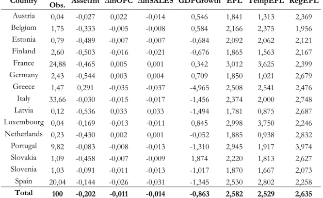
Focusing on Table 1, there is a substantial variation in percentage of observations per country. France and Italy together have more the 50% of the total observations, followed by Spain with 20% of the observations. That is why we present in Section 5 a robustness check where we discard France and Italy data from our sample. The results are similar to our main estimates for H1, but different for H2. Portugal is also well represented in our sample, with 9,82% of the data.

Moreover, the crisis of 2008 is well reflected in the univariate results, because as we can see, the mean of AssetInt, ∆lnOPC, ∆lnSALES and GDPGrowth for most of countries is negative. In fact, the sample period under analysis refers to the years of widespread crisis in the world. As discussed above, countries were not all affected equally by this crisis, and this is also exorbitant in our data. As might be expected, the countries most affected by the crisis are those with the biggest declines, namely in sales and GDP growth. For exemple, Greece has the biggest decline in ∆lnSALES (i.e., 0,035) and between 2008 and 2013 on average the GDP growth was -4,965, followed by Latvia and Italy with -1,494 and -1,456, respectively. Therefore, these numbers reinforce the importance of using our Troika´s variable and corroborate what happened, it could be said that these variables have economic significance. In addition, the variation of ∆lnOPC and ∆lnSALES is similar for most of countries however the correlation between them is 0,841 that is high but not perfect, which indicates stickiness.

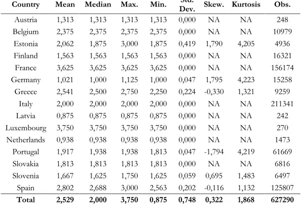
24 Finally, H1 implies differences in EPL indexes, that range from 0 to 6 where 6 represents the strictest EPL. In our sample, the mean EPL is 2, 582 which indicates that our countries are moderated, however, there is a considerable variation in overall EPL strictness. The Portugal, Luxembourg and France have the highest scores (2,945, 2,998 and 3,012, respectively) whereas Latvia and Austria have the lowest scores (1,781 and 1,841, respectively). The correlation between TempEPL and RegEPL is - 0,416 which means that the correlation is low, besides we can say that countries with stricter EPL for regular workers have greater flexibility EPL for temporary workers. For exemple, Latvia has low EPL for temporary workers (the lowest for our sample, at 0,875 which is lower than the median 2) but features stricter EPL for regular workers (at 2,687 which is higher than the median 2,468). On the other hand, Luxembourg has below-median EPL for regular workers (2,246) but has the strictest EPL for temporary workers (3,75).

Table 1: Summary Statistics

Country _Obs. % of AssetInt ∆lnOPC ∆lnSALES GDPGrowth EPL TempEPL RegEPL

Austria 0,04 -0,027 0,022 -0,014 0,546 1,841 1,313 2,369 Belgium _{1,75 -0,333 -0,005 -0,008 0,584 2,166 2,375 1,956} Estonia 0,79 -0,489 -0,007 -0,007 -0,684 2,092 2,062 2,121 Finland _{2,60 -0,503 -0,016 -0,021 -0,676 1,865 1,563 2,167} France _{24,88 -0,465 0,005 0,001 0,342 3,012 3,625 2,399} Germany 2,43 -0,544 0,003 0,004 0,709 1,850 1,021 2,679 Greece _{1,47 0,291 -0,035 -0,037 -4,965 2,508 2,541 2,476} Italy 33,66 -0,030 -0,015 -0,017 -1,456 2,374 2,000 2,748 Latvia 0,12 -0,536 0,033 0,033 -1,494 1,781 0,875 2,687 Luxembourg 0,04 -0,169 -0,013 -0,011 0,845 2,998 3,750 2,246 Netherlands 0,23 -0,430 0,002 0,001 -0,052 1,885 0,938 2,832 Portugal _{9,82 -0,083 -0,008 -0,013 -1,310 2,945 1,917 3,974} Slovakia _{1,09 -0,458 -0,007 -0,009 1,874 2,220 1,813 2,627} Slovenia 1,03 -0,091 -0,011 -0,013 -1,017 1,870 1,667 2,073 Spain _{20,04 -0,144 -0,026 -0,031 -1,345 2,530 2,802 2,258} Total 100 -0,202 -0,011 -0,014 -0,863 2,582 2,529 2,635

AssetInt is defined as 𝑙𝑛 (_{𝑆𝑎𝑙𝑒𝑠 𝑅𝑒𝑣𝑒𝑛𝑢𝑒}𝑇𝑜𝑡𝑎𝑙 𝐴𝑠𝑠𝑒𝑡 ), ∆lnOPC is the first difference of the logarithm of operational costs, ∆lnSALES is the first difference of logarithm of sales revenue, GDPGrowth is defined as the annual percentage growth rate of GDP at market prices based on constant local currency, EPL is the aggregate index of employment protection legislation, computed as the mean of TempEPL (an index of employment protection legislation for temporary employees) and RegEPL (an index of employment protection legislation for regular employees). The sample includes companies for the 15 Euro Area countries and the sample period is from 2008 to 2013.

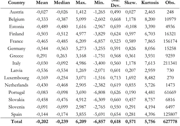
25 Table 2: Descriptive Statistics per Variable

Table 2 Panel A AssetInt defined as ln((Total Asset)/(Sales Revenue))

Country Mean Median Max. Min. _Dev. Std. Skew. Kurtosis Obs.

Austria -0,027 -0,026 1,412 -1,265 0,490 0,027 2,465 248 Belgium -0,333 -0,387 5,099 -2,602 0,668 1,178 8,200 10979 Estonia -0,489 -0,480 1,616 -2,967 0,659 -0,108 3,390 4936 Finland -0,503 -0,512 4,977 -3,829 0,624 0,597 6,703 16321 France -0,465 -0,485 6,209 -6,857 0,523 0,589 7,865 156174 Germany -0,544 -0,563 5,273 -3,255 0,591 0,826 8,056 15258 Greece 0,291 0,263 3,168 -1,751 0,568 0,361 3,931 9259 Italy -0,030 -0,092 4,986 -3,400 0,560 1,178 7,613 211341 Latvia -0,536 -0,534 1,269 -2,071 0,601 0,207 2,959 730 Luxembourg -0,169 -0,254 3,071 -1,516 0,713 1,692 8,482 270 Netherlands -0,430 -0,468 2,905 -2,382 0,619 0,855 5,726 1473 Portugal -0,083 -0,098 3,690 -6,808 0,626 0,190 4,481 61669 Slovakia -0,458 -0,476 4,912 -6,309 0,660 0,457 8,757 6816 Slovenia -0,091 -0,099 2,987 -2,765 0,550 0,291 4,194 6497 Spain -0,144 -0,174 3,855 -5,691 0,654 0,281 4,396 125807 Total -0,202 -0,239 6,209 -6,857 0,618 0,571 5,756 627778

As we can see in Table 2 panel A, the average for AssetInt is negative for all countries of our sample, excepted Greece. A negative ln ( Total Asset

Sales Revenue) means that Total Assets is less

than Sales Revenue, because for a logarithm to be negative, the value to logarithmize must be less than 1. Usually, it is said that this type of firm generates a lot of revenue with little investment and so have a higher associated risk. However, we cannot conclude anything about the performance of our sample, because we only have one ratio. Therefore, it seems to us hasty to draw conclusions about the companies considering the information we have, since the interpretation of a unique ratio can skew our conclusions. In order to understand exactly the performance of the companies, a more in-depth analysis would be necessary, which does not fit directly in the scope of our work.

26 Table 2 Panel B: ∆lnOPC defined as the first difference of the logarithm of

operational costs

Country Mean Median Max. Min. _{Dev. Skew. Kurtosis Obs.} Std.

Austria 0,022 0,006 0,633 -0,383 0,169 0,606 3,921 206 Belgium -0,005 0,000 0,702 -0,752 0,135 -0,203 4,135 9139 Estonia -0,007 0,000 0,870 -0,744 0,175 -0,142 3,821 4110 Finland -0,016 -0,012 1,177 -0,985 0,161 -0,109 4,178 13584 France 0,005 0,006 0,934 -1,113 0,129 -0,093 4,688 130114 Germany 0,003 0,009 0,873 -0,632 0,144 -0,254 3,729 12675 Greece -0,035 -0,029 0,634 -0,766 0,157 -0,068 3,558 7708 Italy -0,015 -0,011 0,957 -1,113 0,161 -0,122 3,756 175935 Latvia 0,033 0,035 0,491 -0,556 0,160 -0,165 3,241 608 Luxembourg -0,013 -0,014 0,328 -0,630 0,147 -0,438 4,060 225 Netherlands 0,002 0,005 0,565 -1,166 0,153 -0,925 8,838 1220 Portugal -0,008 -0,007 1,088 -1,168 0,154 -0,067 4,056 51368 Slovakia -0,007 -0,003 0,970 -1,068 0,175 -0,140 4,266 5676 Slovenia -0,011 -0,008 0,617 -0,692 0,161 -0,088 3,233 5405 Spain -0,026 -0,021 1,266 -1,446 0,160 -0,085 3,904 104812 Total -0,011 -0,006 1,266 -1,446 0,152 -0,140 4,075 5227851 According to Table 2 panel B, and although we use the logarithm, there are still some cross-countries differences in ∆lnOPC that ranges from -0,035 in Greece to 0,033 in Latvia. The countries of southern Europe have a larger negative mean for this variable than the rest of countries, as expected, once the crisis of 2008 had a brutal impact particularly in these economies. Besides, it is important to note that for all countries of our sample, the maximum value is positive, which means that at least for one year, the operational costs have increased. Interestingly, the countries that reached higher values were Finland, Portugal and Spain.

So, these negative values show clearly the impact of the crisis. It is legitimate to argue that a decrease of operational costs can be interpreted as efficiency gains, however almost every country has negative values, which means that happened something on a global scale, that is, a crisis.

1 _{The number of observations for ∆lnOPC is 522 785, because this variable is the first difference of the}

logarithm, so the year 2008 is “lost”. There are 104 993 observations per year, so 5220785+1040993=627778, the total number of observations referred in section 3.2.

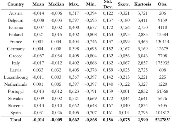
27 Table 2 Panel C: ∆lnSALES defined as the first difference of the logarithm of sales revenue

Country Mean Median Max. Min. _Dev. Std. Skew. Kurtosis Obs.

Austria -0,014 -0,006 0,317 -0,394 0,122 -0,321 3,721 206 Belgium -0,008 -0,003 0,397 -0,595 0,137 -0,180 3,411 9139 Estonia -0,007 -0,002 0,400 -0,677 0,172 -0,126 2,750 4110 Finland -0,021 -0,015 0,402 -0,808 0,163 -0,093 2,885 13584 France 0,001 0,004 0,404 -0,746 0,137 -0,099 3,463 130114 Germany 0,004 0,008 0,398 -0,695 0,152 -0,167 3,169 12675 Greece -0,037 -0,034 0,405 -0,804 0,162 -0,056 3,046 7708 Italy -0,017 -0,012 0,402 -0,868 0,162 -0,067 2,857 175935 Latvia 0,033 0,032 0,405 -0,378 0,159 -0,025 2,725 608 Luxembourg -0,011 0,003 0,367 -0,397 0,142 -0,213 3,221 225 Netherlands 0,001 0,005 0,397 -0,397 0,140 -0,122 3,327 1220 Portugal -0,013 -0,012 0,623 -0,791 0,159 -0,001 2,852 51368 Slovakia -0,009 -0,002 0,521 -0,669 0,172 -0,044 2,641 5676 Slovenia -0,013 -0,010 0,662 -0,648 0,167 -0,040 2,834 5405 Spain -0,031 -0,026 0,405 -0,707 0,161 0,014 2,795 104812 Total -0,014 -0,009 0,662 -0,868 0,156 -0,075 2,990 5227852 Table 2 panel C presents some descriptive statistics for ∆lnSALES. The analysis is like what we have done before. First, there are some cross-countries differences, where Greece has, once again, the lowest value (-0,037) and Latvia has the highest one (0,033). Indeed, when we put the countries ordered from the lowest value to the highest, either in the ∆lnOPC or in the ∆lnSALES, the order does not change, except for Austria, Luxembourg and Estonia. This means that those who see their sales decline tend to decrease operating costs albeit not being in the same proportion. This fact shows us that in certain situations the costs are sticky, which is consistent with ABJ and other authors referred to in literature review.

2 _{The number of observations for ∆lnSALES is 522 785, because this variable is the first difference of the}

logarithm, so the year 2008 is “lost”. There are 104 993 observations per year, so 5220785+1040993=627778, the total number of observations referred in section 3.2.