Testing the Asymmetry of Shocks with Euro Area

(1)

Testing the Asymmetry of Shocks with Euro Area

Marius-Corneliu MARINAŞ Bucharest Academy of Economic Studies

marinasmarius@yahoo.fr

Abstract.The objective of this study is to identify the demand and supply shocks affecting 13 EU member states and to estimate their degree of correlation with the Euro area shocks. This research ensures identifying the asymmetry of shocks degree with the monetary union, depending on which it’s judging the desirability of adopting a single currency. The analysis is also useful for the economies outside the Euro area, because they are strongly commercial and financial integrated especially with the core economies from union. Applying the Blanchard and Quah methodology to estimate the shocks in the period from 1998:1-2010:3, I have found a weak and negative correlation between demand shocks and a medium to high correlation of the supply shocks. The results obtained suggest the presence of a structural convergence process with the Euro area, in the context of domestic macroeconomic policies rather different, both inside and outside the monetary union.

Keywords: demand shocks; supply shocks; SVAR model; Euro area; asymmetric shocks.

JEL Codes: E32, E37. REL Codes: 9B, 9G.

(2)

Introduction

Adopting the Euro entails giving up two instruments that can be used to neutralize macroeconomic shocks. These shocks will become more rather asymmetric, given that there are significant differences with the Euro area's economic structure or it is promoting divergent macroeconomic policies than this. The event of asymmetric shocks will generate a lower correlation of business cycles, increasing the costs of participating in monetary union. To identify the relationship between economic shocks and business cycles, the economic literature is using several methods of the shocks decomposition that affect some nominal and real variables. The most used methodology is that of Blanchard and Quah (1989), further developed by Bayoumi (1991) and Bayoumi and Einchengreen (1992). This concerns the decomposition of the shocks that affects output and inflation in aggregate demand, respectively aggregate supply shocks. This methodology is useful to analyse the risks of a common currency adopting, because it allows identifying the nature of shocks and the most appropriate answers to their action. Bayoumi and Einchengreen have investigated two types of shocks with two type VAR models, one for real GDP and the other for the GDP deflator. The shocks were estimated based on residuals of the two models, with the restrictions specified in the next section of the paper.

The two economists have estimated that for the EU countries there are more asymmetric shocks than US regions, this situation leading to difficulties for stability of the European Monetary Union. Moreover, the shocks adjustment is more difficult in European countries, which will lead to the persistence of high unemployment following a restrictive shock. The methodology was used to estimate the impact of enlargement of monetary union with countries from Central and Eastern Europe. Using data for ten economies from this region and the Euro area economy, Fidrmuc and Korhonen (2001) estimated that Hungary, Latvia and Estonia registered a high supply side shocks correlation with EMU in the period 1994-2000. For others countries the correlation of shock was close to zero, suggesting reduced structural convergence of these countries with EMU. Correlation of shocks on the demand side is generally lower than the supply side, low levels of correlation coefficient reflecting the macroeconomic differences during the transition.

(3)

registered the strongest correlation of shocks on the demand side with the Euro area. Frenkel and Nickel (2002) concluded that there are significant differences between the nature, intensity and capacity of the shock adjustment between CEE countries and the Euro area, but some of the new member states there are similarities with economies within the monetary union. According to Babetski (2003), lower correlation of demand and supply shocks monetary union economies should not be a cause for concern because the situation might improve inside the Euro area. Adapting the endogenous hypothesis of an optimum currency area, the economist showed that Euro adopting for some new member states would lead to increase of the intra-industry trade and greater convergence of demand shocks. Arfa (2009) found that several new member countries of the European Union have a quite high correlation of demand shocks with the Euro area however supply shocks are asymmetric. Socol and Soviani (2010), respectively Socol and Măntescu (2011), have explained the weak correlation of the demand shocks due to differences between national fiscal policies.

A short description of the methodology

The decomposition of the demand and supply shocks involves using a structural type of the VAR model, whose restriction are inspired by traditional macroeconomic model with aggregate demand, short-run aggregate supply and long-run aggregate supply. In the short term, an increase in aggregate demand leads to an increase of both production and inflation, so that there will be a direct relationship between these variables. In the long term, a positive demand shock will generate only an increase in prices, while production volume is constant. Increasing short-run aggregate supply leads to economic growth and to inflation rate reducing, so that there will be an inverse relationship between these variables.

In the VARtypemodels the shocks are a partofavariablethatcannotbe explained byits past values orother variablesincluded inthe model. Thus, the term appears as a shock error (residual) from a certain stochastic equation. To identify demand and supply shocks is used a VAR-type model with two variables (GDP and inflation rate) which can be writtenas in the equations (1) and (2), where each variable is influencedbyactual andlagged values of other variables and by its lagged values.

t y t t

t

t b b ir c y c ir e

y = ₁₀ − ₁₂ × + ₁₁× ₋₁+ ₁₂× ₋₁ + _, (1)

t ir t t

t

t b b y c y c ir e

(4)

Where variables yt şi irt are supposed to be stationary, ey,tşi eir,t represents

the errors with standard deviations σyşi σir, which are not correlated.

BlanchardandQuahdirectlyassociatedstructuralshocks of demand (εdt)

and supply (εst) with yt and irt variables, as a bivariate moving average. The

vector (Xt) composed by the two endogenous variables will be written as an

infinite moving average vector of structural shocks, including demand and supplyshocks: t n n n n t n t t

t C C C L C

X = ×ε + ×ε + ×ε =

∑

×ε

∞ = − − 0 1 1

0 ... (3)

where _⎥

⎦ ⎤ ⎢ ⎣ ⎡ = st dt t _ε ε

ε and L is a lag operator; L0εt= εt; L1εt= εt-1; L2εt= εt-2....

The starting point of their model is the following:

⎥ ⎦ ⎤ ⎢ ⎣ ⎡ × ⎥ ⎦ ⎤ ⎢ ⎣ ⎡ = ⎥ ⎦ ⎤ ⎢ ⎣ ⎡

∑

∞ = st dt

i i i

i i t t a a a a ir y ε ε Δ Δ

0 21 22

12 11

(4)

where Δyt and Δirt represent, respectively, changes in the logarithm of output

and prices at time t, εdt and εst represent supply and demand shocks and akji

represent each of the elements of the impulse-response function to shocks.

The model defined by equations (4) also implies that the bivariate endogenous vector can be explained by lagged values of every variable. If Ai

represents the value of model coefficients, the model to be estimated is the following: ⎥ ⎦ ⎤ ⎢ ⎣ ⎡ + + ⎥ ⎦ ⎤ ⎢ ⎣ ⎡ × + ⎥ ⎦ ⎤ ⎢ ⎣ ⎡ × = ⎥ ⎦ ⎤ ⎢ ⎣ ⎡ − − − − irt yt t t t t t t e e ir y A ir y A ir y ... 2 2 2 1 1 1 _Δ Δ Δ Δ Δ Δ

, (5)

where eyt and eirt are the residuals of every VAR equation. Equation (5) can be

also expressed as:

⎥ ⎦ ⎤ ⎢ ⎣ ⎡ × + + + = ⎥ ⎦ ⎤ ⎢ ⎣ ⎡ × − = ⎥ ⎦ ⎤ ⎢ ⎣ ⎡ ₋ irt yt irt yt t t e e L A L A I e e L A I ir Y ...) ) ( ) ( ( )) (

( 1 2

Δ Δ

, (6)

and in an equivalent manner:

⎥ ⎦ ⎤ ⎢ ⎣ ⎡ × ⎥ ⎦ ⎤ ⎢ ⎣ ⎡ = ⎥ ⎦ ⎤ ⎢ ⎣ ⎡

∑

∞ = irt yt

i i i

i i t t e e d d d d ir Y

0 21 22

12 11

Δ Δ

(7)

(5)

⎥ ⎦ ⎤ ⎢ ⎣ ⎡ × ⎥ ⎦ ⎤ ⎢ ⎣ ⎡ × = ⎥ ⎦ ⎤ ⎢ ⎣ ⎡ × ⎥ ⎦ ⎤ ⎢ ⎣ ⎡

∑

∞ = ∞ = st dt

i i i

i i i irt

yt

i i i

i i a a a a L e e d d d d ε ε

0 21 22

12 11

0 21 22

12 11

, (8) Where a matrix, denoted by c, can be found that relates demand and supply shocks with the residuals from the VAR model.

⎥ ⎦ ⎤ ⎢ ⎣ ⎡ × = ⎥ ⎦ ⎤ ⎢ ⎣ ⎡ × ⎥ ⎥ ⎦ ⎤ ⎢ ⎢ ⎣ ⎡ ⎥ ⎦ ⎤ ⎢ ⎣ ⎡ × × ⎥ ⎦ ⎤ ⎢ ⎣ ⎡ = ⎥ ⎦ ⎤ ⎢ ⎣ ⎡

∑

∞ = − ∞ = st dt st dt

i i i

i i irt yt c a a a a L d d d d e e ε ε ε ε

0 21 22

12 11 1

0 21 22

12 11

. (9)

From equation (9) it results that in the 2x2 considered model, four restrictions are needed to define uniquely the four elements of matrix c. Two of these restrictions are simple normalisations that define the variances of shocks εdt and εst. The usual convention in VAR models consists of imposing the two

variances equal to one, which together with the assumption of orthogonality define the third restriction c’×c=Σ, where Σ is the covariance matrix of the residuals ey and eir. The final restriction that permits matrix c to be uniquely

defined comes from macroeconomic theory and it refers to cumulative effects of demand shocks on output which must be zero.

Results obtained

In this study I have applied SVAR methodology to identify aggregate demand and supply shocks for 13 economies of the EU and the Euro area. Five of the economies are from Central and Eastern Europe (Romania, Hungary, Czech Republic, Poland, Slovakia), four are peripheral (Portugal, Spain, Greece and Ireland) and others are form the euro area core (Germany, France, Italy and Austria). Motivation for choosing these economies was that of estimating the degree of the shocks correlation within the euro area (between core and periphery) and between several new member states and the Euro area as a whole, respectively some economies that form it. To identify the demand and supply shocks I have used quarterly data series of real GDP and inflation in the period 1998:1 - 2010:3, the total number of observations being 51. Real GDP was expressed as an index with base year 2000, while inflation is the percentage change in GDP deflator. The source of data was Eurostat and to estimate the demand and supply shock I have used EViews software. Because of the influence of seasonality specific to quarterly macroeconomic data, I have applied for all data series of TRAMO/SEATS to eliminate this feature of the variables.

(6)

the presence of a trend or lack of stationarity. To investigate this hypothesis, I have used the ADF test, whose H0 hypothesis is the existence of a unit root. For most data series I have estimated the existence of a unit root at level and no root on the first differences. It results that the variables are integrated of order 1, ie I (1). In the table below I have included the probabilities associated with the ADF test for I (0) and for I (1). If the probability is higher than threshold of significance (5%, respectively 1%) then that variable has not stationary.

According to the results of the stationarity test included in Table 1, Ireland is the only economy whose GDP is stationary at the level, evidence of an economy flexible, easily able to neutralize the shocks affecting it. Hungary and Slovakia register also a relatively high level of economic flexibility. In terms of inflation, it is stationary at 1% in Germany and Slovakia, proving the ability of domestic supply side to counteract the influence of aggregate demand shocks. Furthermore, the stationarity at level is a virtue in a monetary union, allowing faster adjustment of economic shocks that generate either a decline in the economy or is overheating it.

Table 1 The ADF test probabilities

Countries GDP GDP DEFLATOR

I(0) I(1) I(0) I(1)

H0: There is a unit root (it’s lacking stationarity)

Romania 0.8544 0.0072 0.5854 0.0000

Euro Area 0.5386 0.0005 0.4605 0.0000

Germany 0.1864 0.0000 0.0042 -

France 0.2034 0.0014 0.2825 0.0001

Italy 0.2028 0.0005 0.7892 0.0000

Austria 0.6111 0.0108 0.8829 0.0001

Spain 0.9863 0.0026 0.1065 0.0001

Portugal 0.1377 0.0000 0.0409 0.0000

Greece 0.2265 0.0000 0.1197 0.0000

Ireland 0.0110 0.0000 0.7982 0.0000

Czech Republic 0.2388 0.0169 0.1823 0.0000

Hungary 0.0871 0.0002 0.0424 0.0000

Poland 0.7708 0.0128 0.1075 0.0000

Slovakia 0.1368 0.0000 0.0028 -

Source: Eurostat (2011); personal estimations with Eviews 7 software.

Since the variables expressed as first differences became stationary, I have built one VAR model consists of real GDP and inflation series for each of the 14 economies. A VAR model is valid if it satisfies the following conditions: a good representation of the model, by choosing the optimal number of

(7)

stability, obtained if the roots are lower than unity;

residual validity by lack of autocorrelation, by normalization and homoskedasticity.

To identify the correct number oflags of the VAR model for economies included in this paper I have used the criteriaprovidedby LRSequential tests, Akaike Criterion, Schwarz and Hanna-Quinn Criterion tests. To validate these tests I have applied the Lag Exclusion Wald Test, whose null hypothesis is rejecting the choice lag. If its probability is below 1% or 5% the optimal lag is selected. According to the results included in the Table 2, it results that eight economies have a VAR with one lag, three have VAR models with two lags and another three are characterized by 3 and 4 lags for the two data sets included the VAR.

Table 2 The estimation of the number of VAR lags

Countries Sequential

LR AIC SC HQ

Chosen lag

Probabilities of Lag exlusion test H0:

the statistics χ2

rejects the selected lag

Romania 4 4 4 4 4 0.000261

Euro Area 1 1 1 1 1 0.000136

Germany 1 1 1 1 1 0.033883

France 2 3 1 2 2 0.039302

Italy 1 1 1 1 1 0.000214

Austria 1 1 1 1 1 0.000796

Spain 4 4 1 4 4 0.003020

Portugal 2 2 2 2 2 0.027871

Greece 3 3 3 3 3 0.027798

Ireland 1 1 1 1 1 0.000000

Czech Republic 1 1 1 1 1 0.000053

Hungary 1 1 1 1 1 0.007902

Poland 2 2 1 2 2 0.009867

Slovakia 1 1 1 1 1 0.000000

(8)

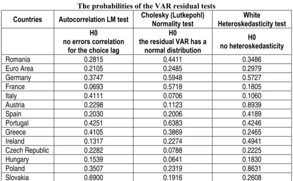
Table 3 The probabilities of the VAR residual tests

Countries Autocorrelation LM test Cholesky (Lutkepohl) Normality test

White

Heteroskedasticity test H0

no errors correlation for the choice lag

H0

the residual VAR has a normal distribution

H0

no heteroskedasticity

Romania 0.2815 0.4411 0.3486

Euro Area 0.2105 0.2485 0.2979

Germany 0.3747 0.5948 0.5727

France 0.0693 0.5718 0.1805 Italy 0.4111 0.0706 0.1060 Austria 0.2298 0.1123 0.8939 Spain 0.2030 0.2006 0.4189

Portugal 0.4251 0.6383 0.4246

Greece 0.4105 0.3869 0.2465 Ireland 0.1317 0.2274 0.4941

Czech Republic 0.2282 0.0788 0.2225

Hungary 0.1539 0.0641 0.1830

Poland 0.3507 0.2319 0.8631

Slovakia 0.6900 0.1916 0.2608

Once I have established the final form of VAR models and have checked their statistical validity, I imposed structural restrictions needed to identify the demand and aggregate supply shocks. To achieve compatibility between the theoreticalmodel(aggregate demand –aggregate supply) andSVARmodel, the latter must meetthe followingconditions:

Aggregate demand shocks on GDP are some temporary, while aggregate supply shocks are some permanently. Therefore, the accumulated response of economic growth rate to aggregate demand shocksshould register a neutralization, whilethe response toaggregate supply shockispermanent. In other words, an aggregate demand shock has only temporary and positive influence on output.

(9)

growth. Thus, a shock of 1% of the aggregate supply led to increase of real GDP by 0.17% standard deviation in the first quarter in Slovakia and by 0.2% after 10 quarters. In Greece, the increase was about 0.1% on short term and over 0.3% after nine quarters.

Among the new EU countries, Romania was characterized by largest long-term effect of supply shocks on economic growth (about 0.3% standard deviation). In the case of other new EU member states included in the analysis (Hungary, Czech Republic, Poland), GDP change was at least 0.12% after 10 quarters. Among the countries from the Euro area, Spain has registered a GDP change by about 0.16%, following a positive supply shock with one point standard deviation, while the GDP of Germany, Italy and Ireland have increased by approximately 0.14%. Generally, relatively less developed economies than in Euro area core countries have a greater potential for growth, feature corresponding to decreasing marginal returns hypothesis. The aggregate demand shocks had a temporary feature, so they are neutralized after two quarters in Hungary, three quarters in Slovakia and after five quarters in the Euro area. In Ireland and Italy, demand shocks exert a negligible impact on economic growth. Romania has registered the highest period in which a demand shock is active, it neutralizing after approximately five years.

.000 .005 .010 .015 .020 .025 .030

1 2 3 4 5 6 7 8 9 10 Demand shock Supply shock Accumulated Response of Dlog (ROMANIA). GDP to Structural

One S.D. Innovations

-.002 .000 .002 .004 .006 .008 .010 .012 .014

1 2 3 4 5 6 7 8 9 10 Demand shock Supply shock Accumulated Response of Dlog (EURO AREA). GDP to Structural

-.002 .000 .002 .004 .006 .008 .010 .012 .014

1 2 3 4 5 6 7 8 9 10 Demand shock Supply shock

Accumulated Response of Dlog (AUT).GDP to Structural One S.D. Innovations

.000 .004 .008 .012 .016 .020

1 2 3 4 5 6 7 8 9 10 Demand shock Supply shock Accumulated Response of Dlog (CZECH). GDP to Structural

-.002 .000 .002 .004 .006 .008 .010

1 2 3 4 5 6 7 8 9 10 Demand shock Supply shock Accumulated Response of Dlog (FRANCE). GDP to Structural

.000 .002 .004 .006 .008 .010 .012 .014 .016

1 2 3 4 5 6 7 8 9 10

Demand shock Supply shock Accumulated Response of Log (GERMANY). GDP to Structural

(10)

-.005 .000 .005 .010 .015 .020 .025 .030 .035

1 2 3 4 5 6 7 8 9 10

Demand shock Supply shock Accumulated Response of Dlog (GREECE). GDP to Structural

.00 .02 .04 .06 .08 .10 .12 .14 .16

1 2 3 4 5 6 7 8 9 10

Demand shock Supply shock Accumulated Response of Log (IRELAND). GDP to Structural

.000 .002 .004 .006 .008 .010 .012 .014 .016

1 2 3 4 5 6 7 8 9 10

Demand shock Supply shock Accumulated Response of Dlog (ITALY). GDP to Structural

.000 .002 .004 .006 .008 .010 .012 .014

1 2 3 4 5 6 7 8 9 10

Demand shock Supply shock Accumulated Response of Dlog (POLAND). GDP to Structural

.003 .004 .005 .006 .007 .008

1 2 3 4 5 6 7 8 9 10

Demand shock Supply shock Accumulated Response of Dlog (PORTUGAL). GDP to Structural

-.004 .000 .004 .008 .012 .016 .020 .024

1 2 3 4 5 6 7 8 9 10 Demand shock Supply shock Accumulated Response of Dlog (SLOVAKIA). GDP to Structural

.000 .004 .008 .012 .016 .020

1 2 3 4 5 6 7 8 9 10

Demand shock Supply shock Accumulated Response of Dlog (SPAIN). GDP to Structural

.000 .004 .008 .012 .016 .020

1 2 3 4 5 6 7 8 9 10

Demand shock Supply shock Accumulated Response of Dlog (HUNGARY). GDP to Structural

Figure 1. Accumulated responses of GDP to demand and supply shocks

(11)

.00 .01 .02 .03 .04 .05 .06 .07 .08

1 2 3 4 5 6 7 8 9 10 Demand shock Supply shock Accumulated Response of Dlog (ROMANIA).INFLATION to Structural

-.001 .000 .001 .002 .003

1 2 3 4 5 6 7 8 9 10 Demand shock Supply shock Accumulated Response of Dlog (EURO AREA). INFLATION to Structural

-.001 .000 .001 .002 .003 .004

1 2 3 4 5 6 7 8 9 10 Demand shock Supply shock Accumulated Response of Dlog (AUT).INFLATION to Structural

-.004 -.002 .000 .002 .004 .006 .008 .010

1 2 3 4 5 6 7 8 9 10 Deamnd shock Supply shock Accumulated Response of Dlog (CZECH).INFLATION to Structural

-.002 -.001 .000 .001 .002 .003 .004 .005

1 2 3 4 5 6 7 8 9 10 Demand shock Supply shock Accumulated Response of Dlog (FRANCE). INFLATION to Structural

-.002 -.001 .000 .001 .002 .003 .004

1 2 3 4 5 6 7 8 9 10

Demand shock Supply shock Accumulated Response of Log (GERMANY). INFLATION to Structural

.000 .001 .002 .003 .004 .005 .006 .007

1 2 3 4 5 6 7 8 9 10 Demand shock Supply shock Accumulated Response of Dlog (GREECE).INFLATION to Structural

-.002 .000 .002 .004 .006 .008 .010 .012 .014

1 2 3 4 5 6 7 8 9 10 Demand shock Supply shock Accumulated Response of Dlog (IRELAND).INFLATION to Structural

-.003 -.002 -.001 .000 .001 .002 .003 .004 .005

1 2 3 4 5 6 7 8 9 10 Demand shock Supply shock Accumulated Response of Dlog (ITALY).INFLATION to Structural

-.008 -.004 .000 .004 .008 .012

1 2 3 4 5 6 7 8 9 10 Demand shock Supply shock Accumulated Response of DLOG (POLAND).INFLATION to Structural

-.02 -.01 .00 .01 .02 .03 .04

1 2 3 4 5 6 7 8 9 10 Demand shock Supply shock Accumulated Response of Dlog (PORTUGAL).INFLATION to Structural

-.004 .000 .004 .008 .012 .016

1 2 3 4 5 6 7 8 9 10 Demand shock Supply shock Accumulated Response of Dlog (SLOVAKIA).NFLATION to Structural

(12)

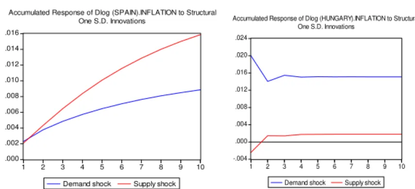
.000 .002 .004 .006 .008 .010 .012 .014 .016

1 2 3 4 5 6 7 8 9 10 Demand shock Supply shock Accumulated Response of Dlog (SPAIN).INFLATION to Structural

-.004 .000 .004 .008 .012 .016 .020 .024

1 2 3 4 5 6 7 8 9 10

Demand shock Supply shock Accumulated Response of Dlog (HUNGARY).INFLATION to Structural

Figure 2. Accumulated responses of inflation rate to demand and supply shocks

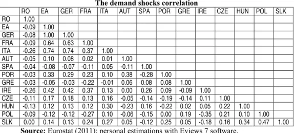
It results that this analysis confirmed the importance of supply shocks impact on economic growth and demand for inflation control, supposing that long-term impact of demand on output is neutralizes. To identify the relationship between the intensity of shocks affecting the economies included in this study, we used Pearson correlation coefficient. According to the results obtained and included in tables 4 and 5, joining to the Euro area did not reduce the risk of asymmetric shocks in the event of periphery economies monetary union. The core of it is relatively strongly correlated with the supply side both the whole Euro area, as well as inside it. Among the peripheral countries, Ireland and Portugal had supply and demand shocks positively correlated with the core Euro area, while Spain and Greece have promoted divergent macroeconomic policies in relation to monetary union. For most economies, the correlation of the shocks on the demand side is lower than the supply ones. The weak correlation of demand shocks can be explained by:

Differences between economic, trade and financial structures of the two economies.

The existence of different exchange rate regimes and different rates of inflation.

Differences between stages of development.

Promoting divergent macroeconomic policies, as a result of different economic developments.

(13)

Table 4 The demand shocks correlation

RO EA GER FRA ITA AUT SPA POR GRE IRE CZE HUN POL SLK RO 1.00

EA -0.09 1.00

GER -0.08 1.00 1.00

FRA -0.09 0.64 0.63 1.00

ITA -0.26 0.74 0.74 0.37 1.00

AUT -0.05 0.10 0.08 0.02 0.01 1.00

SPA -0.04 -0.08 -0.07 -0.11 0.05 -0.11 1.00 POR -0.03 0.33 0.29 0.23 0.10 0.38 -0.28 1.00 GRE -0.03 -0.05 -0.03 -0.22 -0.01 0.06 0.08 0.08 1.00

IRE -0.26 0.42 0.42 0.37 0.13 0.00 0.26 0.09 -0.09 1.00 CZE -0.11 0.17 0.18 0.13 0.16 -0.05 -0.14 -0.19 -0.14 0.11 1.00 HUN -0.13 0.12 0.13 0.12 0.30 -0.23 0.16 -0.22 0.02 0.05 0.22 1.00 POL -0.09 -0.12 -0.12 -0.27 0.10 -0.06 -0.15 0.00 0.19 -0.35 0.21 0.10 1.00 SLK 0.00 0.14 0.13 0.24 0.27 0.05 -0.12 0.25 0.05 -0.18 0.16 0.34 0.47 1.00

Among the new EU member states, Czech Republic, Slovakia and Hungary showed a positive correlation of the demand shocks with the Euro area, but weaker as significance, while Poland and Romania had a divergent evolution with the monetary union. Between four of the five CEE economies (except Romania) there was a trend in the same sense of demand shocks. This group of economies has been characterized by a process of structural convergence with EU economies and integration through trade with them, which was reflected in a positive synchronization of the supply shocks with those economies. Hungary, Romania and Slovakia are the most synchronized with the Euro area while the second economy has the most correlated supply shocks with the rest of the economy within the same group.

Table 5 The supply shocks correlation

RO EA GER FRA ITA AUT SPA POR GRE IRE CZE HUN POL SLK

RO 1.00

EA 0.54 1.00

GER 0.55 1.00 1.00 FRA 0.40 0.75 0.74 1.00 ITA 0.55 0.78 0.78 0.55 1.00 AUT -0.64 -0.57 -0.55 -0.25 -0.53 1.00 SPA 0.70 0.60 0.61 0.41 0.49 -0.59 1.00 POR 0.19 0.32 0.33 0.26 0.23 -0.25 0.09 1.00 GRE 0.23 0.27 0.25 0.28 0.17 -0.09 0.09 0.02 1.00 IRE 0.40 0.45 0.44 0.43 0.46 -0.32 0.45 0.05 0.15 1.00 CZE 0.35 0.13 0.15 -0.03 0.10 -0.30 0.16 -0.20 0.05 -0.06 1.00 HUN 0.51 0.58 0.58 0.51 0.51 -0.50 0.39 0.20 0.50 0.29 0.30 1.00 POL 0.43 0.10 0.11 0.10 0.16 -0.21 0.17 -0.03 0.18 0.28 0.31 0.13 1.00 SLK 0.54 0.46 0.46 0.34 0.45 -0.32 0.45 0.11 0.23 0.46 0.06 0.40 0.18 1.00

(14)

To capture the evolution of demand and supply shocks correlation between Romania and the Euro area I have used the five-yearrolling-window correlation of five years method. According to this methodology, it appears that there was a weak connection between demand shocks, which is rather contrary in the case of the two economies. The economic crisis has induced a greater divergence of these shocks, the correlation value being about -0.3. The impact of crisis on supply shocks was a different one, generating the transition from weak correlation (lower than 0.3) during 2003-2008, to the average correlation by 0.7 in 2004-2009. Moreover, the correlation of supply shocks higher (approximately 85%) took place between 2007 and 2009. Therefore, the aggregate supply response in Romania has become more similar to the euro area, something which will ensure a higher symmetry of shocks in the future.

Figure 3. The correlation of demand and supply shocks between Romania and Euro area (5-yearrolling-window correlation)

Conclusion

The methodology applied in this study is a useful framework to analyse the risks of adopting a common currency, because it allows the identification of the nature of the shocks and more appropriate responses to their action. The basic idea is that aggregate demand shocks affect real GDP only short term, while the impact on inflation is one permanently. The aggregate supply shocks have a permanent influence on the short and long term both on prices and production, the relationship between these being one inverse (increasing the aggregate supply increases production and reduce inflation).

-0.40 -0.30 -0.20 -0.10 0.00 0.10 0.20 0.30 0.40 0.50 0.60 070 0.80

2004Q1 2004Q4 2005Q3 2006Q2 2007Q1 2007Q4 2008Q3 2009Q2 2010Q1

(15)

The cumulative reaction of the GDP to aggregate demand and supply shocks respects the theoretically macroeconomic correlations for all 14 economies analyzed. Thus, supply shocks have a permanent impact, while demand-side shocks are insignificant in most cases.

Slovakia has the highest reaction of the GDP in the first quarter of the after the event of a supply shock, while Greece had the highest long-term growth.

Romania was characterized by the largest period when the demand shock is active, neutralizing it after approximately five years.

Regarding to the inflation response to aggregate supply shocks and demand, theoretical correlations were not observed in four out of 14 cases.

Prices of final goods in Romania, Greece, Ireland and Spain have a high degree of rigidity to decrease.

The core of the monetary union is relatively strongly correlated with both the supply side the whole Euro area, as well as inside it. Ireland and Portugal have supply and demand shocks positively correlated with the core Euro area, while Spain and Greece have promoted divergent macroeconomic policies in relation to monetary union. For the most economies, the correlation of the demand shocks is lower

than the supply ones. Hungary, Romania and Slovakia are the most synchronized CEE economies with the Euro area in terms of supply shocks. The correlation of supply shocks is important for a higher synchronization of business cycles in the Euro area.

Aggregate supply response in Romania has become more similar to the Euro area, something which will ensure a higher symmetry of shocks in the future.

Acknowledgements

(16)

References

Arfa, B.N., „Analysis of Shocks Affecting Europe: EMU and some Central and Eastern Acceding Countries”, Panoeconomicus, No. 1, 2009, pp. 1-15

Babetski, J., „EU Enlargement and Endogeneity of some OCA Criteria: Evidence from the CEECs, Czech National Bank”, Working paper, No.2, 2004, pp. 5-20

Bayoumi, T., Eichengreen B. (1992). Shocking Aspects of European Monetary Integration, in: Growth and adjustment in the European Monetary Union, ed. Torres Francisco and Francesco Giavazzi, pp. 193-230, New York: Cambridge University

Blanchard, O.J., Quah, D., „The Dynamic effects of Aggregate demand and Supply

Disturbances”, American Economic Review, 79(4), 1989, pp.655-673

Fidrmuc, J., Korhonen, I., „The Euro goes East. Implications of the 2000-2002 economic

slowdown for synchronisation of business cycles between the euro area and CEECs”, BOFIT, Discussion Paper, No. 6, 2003, pp. 313-334

Frenkel, M., Nickel, Ch, „How Symmetric are the Shocks and the Shocks Adjustment Dynamics between the Euro Area and Central and Eastern Europe?”, IMF Working Paper, 02/222, 2002, pp. 53-74

Ramos, R., Suriach, J., „Shocking Aspects of European Enlargement”, Eastern European Economics, 42(5), 2004, pp. 36-57

Socol, C., Soviani, R., „Experiences of the Large Fiscal Adjustments in EU. Romania’s Case”, Theoretical and Applied Economics, 12(553), 2010, pp. 21-28

Socol, A.G., Măntescu, D., „Re-modeling the Romanian Fiscal Policy under the Terms of the

Economic Crisis”, Theoretical and Applied Economics, 1(554), 2011, pp. 111-120

Weimann, M., „OCA Theory and EMU Eastern Enlargement – An Empirical Application”,

Dresdner Beiträge zur Volkswirtschaftslehre, no. 7, 2002, Technische Universität Dresden, pp. 5-30