FF From Theory to Practice

(1)

FOUNDATION FIELDBUS: FROM THEORY TO PRACTICE

Vítor Viegas

1)

_{, J. M. Dias Pereira}

2)

1)_{Polytechnic Institute of Setúbal, 2910-761 Setúbal, Portugal, vitor.viegas@estsetubal.ips.pt} 2)_{Polytechnic Institute of Setúbal, 2910-761 Setúbal, Portugal, dias.pereira@estsetubal.ips.pt}

Abstract: This paper describes the main characteristics of the Foundation Fieldbus (FF) technology considering both communication levels, namely H1 and H2, which have bit rates of 31.25 K and 100 Mbit/s, respectively. Several details about the physical layer, communication stack and user layer will be highlighted. Topics related with the configuration of instruments, as well as the design and implementation of supervision software, based on a LabVIEW interface, will be presented. A pilot plant that includes temperature, pressure, level and flow variables will be used to test and validate the capabilities of FF systems. Experimental results will be analyzed, their meaning discussed and the overall performance evaluated.

Keywords: Foundation Fieldbus, industrial networks, fieldbus control systems, Open Process Control, supervision, data acquisition.

1. INTRODUCTION

The Foundation Fieldbus (FF) [1-3] is a communication technology intended to connect instruments in a process automation environment. At the physical level, communications are supported by a two-wire, multidrop bus that supplies power and ensures the flow of digital data. At the logic level, communications are supported by a protocol that guarantees message delivery in real-time [4]. On the top of the protocol layers, functional blocks hide communication details and make easier the development of control applications. FF is a broad technology that covers topics such as power over bus, real-time networking, visual programming, and information management.

The FF technology is supervised by the Fieldbus Foundation [5], a non-profit corporation composed by end-users, manufacturers and research organizations. The foundation promotes and regulates the use of the technology and provides guidelines for the future. The regulation work includes rigorous certification programs that guarantee interoperability between equipment from different manufacturers. The goal is to give end-users the ability to choose the best hardware and software at any time without being stuck to a specific vendor.

The FF technology distinguishes between low-speed communications (H1 level) and high-low-speed communications (H2 level) (see figure 1). The H1 level acts as a digital replacement for 4-20 mA current loops widely used in common industrial plants. The

H2 level aggregates data from H1 segments and adds support for discrete control. Together, H1 and H2 levels satisfy the automation needs of most systems whether they are continuous or discrete.

H1 level

Field instruments

Linking Device (LD) Host

+ Configuration tool

Terminator

Discrete IO H2 level

T

... ...

Fig. 1 – FF overview.

1.1. H1 LEVEL

The H1 level is a digital bus that implements a subset of the OSI (Open Systems Interconnection) model. The physical layer is fully implemented, while layers 2 to 7 are compressed in the so-called

“communication stack”. The user layer (extra OSI)

defines a library of functional blocks intended to build control applications. These three components computing@computingonline.net

www.computingonline.net

ISSN 1727-6209

(2)

(physical layer, communication stack and functional blocks) must all reside in every FF instrument.

The physical layer has the following characteristics:

 Power over bus: The bus is powered with 24 VDC and a current capability above 100 mA (typical). Each instrument can draw up to 20 mA from the bus.

 Data rate of 31.25 Kbit/s: The data is transmitted together with the clock, in base band, using Manchester coding. The digital signal is superimposed over the DC level. The relatively low data rate allows the reuse of 4-20 mA wiring.

 Free topology: Spurs are allowed anywhere along the bus. The maximum cable length (including spurs and considering high-quality wiring) is about 1900 m. This value can be extended to 7600 m by adding up to four repeaters. The bus must have a proper RC terminator to avoid signal reflections.

 6, 12 or 32 instruments: The maximum number of instruments is six if bus powered with Intrinsic Safety (IS), 12 if bus powered without IS, and 32 if neither bus powered nor IS. These values are merely indicative since they depend on the actual power specifications of the devices.

The communication stack implements a master-slave protocol that guarantees message delivery in real-time. The master is called “Link Active

Scheduler” (LAS) because it distributes “permissions to talk” (tokens) according a deterministic schedule.

When a device receives the token, it publishes messages on the bus that are picked up and consumed by one or more subscribers. The LAS supports the following dialogues:

 Programmed dialogues: Periodically, according a programmed control strategy, the LAS sends tokens of type CD (Compel Data). The device owning the CD token publishes data immediately without waiting for the subscriber(s) to confirm the reception. If a data point is lost, the system relies on the previous value until a new one is transmitted. This dialogue is used to transfer output variables and status information between functional blocks.

 Unprogrammed dialogues: After executing the control strategy, the LAS reserves some time to send tokens of type PT (Pass Token). The device owning the PT token has a limited amount time to send messages by its own initiative. All messages have to be confirmed otherwise are repeated. This dialogue is used to report events (such as alarms and trends) and to perform configuration tasks

(such as set-point and tuning adjustments, program downloading, and remote diagnostics).

 Live list dialogue: The LAS maintains a list of active devices by sequentially sending tokens of type PN (Probe Node) to all possible addresses (0 to 255). The target device responds by returning its unique IDentifier (ID) and tag number. If a new device is found it is added to the list; if a device fails to respond three consecutive times it is removed from the list.

 Time distribution dialogue: The LAS distributes time by sending tokens of type TD (Time Distribution) to all devices. Each device compares its internal clock against the timestamp received and resets it to maintain accuracy within 1 ms.

Each H1 bus has one primary master. Other devices can be configured as redundant masters provided they have LAS capabilities. The master with lowest address takes control automatically and transparently.

As said before, the programming interface of FF devices is based on functional blocks. Each device contains:

 One Resource Block (RB) that describes the general characteristics of the device (such as ID, tag number, manufacturer, model, serial number, firmware version and available features). This data, which is stored in a non-volatile memory, is very useful for maintenance and inventory purposes.

 One or more Transducer Blocks (TB) that describe the characteristics of primary transducers (such as transducer type, connection, compensation, and calibration data).

 One or more Function Blocks (FB) that implement data processing algorithms. There are dozens of predefined FBs covering the most common functionalities. Some examples are:

– Analog Input (AI): Takes the data from the analog input signal and makes it available to other FBs. It implements scaling conversion, filtering, square root extraction, and alarm processing.

– Analog Output (AO): Provides a real value to generate an analog output signal. It implements value limiting, scaling conversion, and fault-state handling.

– Digital Input (DI): Takes the data from the discrete input signal and makes it available to other FBs. It implements value inversion, filtering and alarm processing.

(3)

implements value inversion and fault state handling.

– Proportional, Integral, Derivative (PID): Implements the PID algorithm with a lot of valuable features such as set-point treatment (value and rate limiting), filtering, feed forward, anti-wind-up and alarm processing.

– Arithmetic (ARTH): Provides some

predefined, ready-to-use equations such as flow compensation, hydrostatic tank gauging, ratio control and others.

– Integrator (INTG): Integrates a variable in function of the time.

– Set-Point Generator (SPG): Generates a set-point following a profile in function of the time.

– TIMEr and logic (TIME): Implements combinational logic and timers.

The control strategy is defined by a FB diagram (see figure 2). The arrows establish data relations between FBs: if two interdependent FBs reside on the same device data is transferred internally; if they reside in different devices data is transferred across the bus. By dissecting the diagram it is possible to know who talks to whom and when; in other words, it is possible to schedule programmed dialogues. Each FB can also be configured individually to determine its behavior in terms of processing and event reporting. It should be noted that by enabling the transmission of alarms and trends the bus gets loaded with unprogrammed dialogues.

The use of predefined FBs promotes interoperability because devices can be replaced while the program maintains the same structure.

SP: Set-Point PV: Process Variable OV: Output Variable

LD

AI

PID

AO PV

SP

OV

T

Fig. 2 – Flow control loop (instruments and FB diagram).

1.2. H2 LEVEL

The H2 level aggregates data from the field including H1 segments, Programmable Logic Controllers (PLC), and sensor buses. Over the last years there has been an effort to apply internet technologies at this level: Ethernet for data transmission, Internet Protocol (IP) for data routing, and Transport Control Protocol (TCP) and User Datagram Protocol (UDP) for data transport. This approach provides high baud rates (100 Mbit/s typical) and allows the use of inexpensive, commercial off-the-shelf equipment. In return, it does not provide native support for real-time, power over bus or redundancy.

Each H1 segment is connected through a gateway

called “Linking Device” (LD), which, most of the

times, acts as the primary master and provides support for discrete control. When the host needs to access a particular H1 device, it sends TCP messages to the corresponding linking device which translates them into H1 dialogues. The reverse happens when the H1 device reports data to the host. UDP messages are used when the host needs to contact several linking devices simultaneously (to distribute time, for example). The process of translation is absolutely transparent so that configuration tools (residing on the host) can configure, diagnose and monitor H1 devices as if they were locally connected.

1.3. FIELDBUS CONTROL SYSTEMS

FF instruments are considered to be “smart”

because they have processing power and can communicate with each other. This allows them to perform identification, diagnostics and self-calibration routines, and, more important, to collaborate in the execution of distributed control

algorithms. The result is a “Fieldbus Control System”

(FCS), so-called because the control strategy is decentralized across the bus. Compared to more conventional architectures, such as Distributed Control Systems (DCS) or Direct Digital Control (DDC) systems [6], the FF technology provides the following advantages:

 Common to FCS systems:

– Extended visibility and smartness: Visibility goes down to primary transducers as opposite to traditional systems where visibility is limited to input/output cards of PLCs and DCSs. Self-describing information and online diagnostics facilitate asset management and maintenance. Robust protocols allow the hot swapping of devices.

(4)

wiring can be reused in most cases.

– Improved robustness: If the primary master fails the secondary master takes control of the bus immediately.

 Specific to the FF technology:

– Interoperability: Rigorous certification programs, supported by a strong community, guarantee interoperability between equipment from different manufacturers.

– Productivity: The programming model based on standard functional blocks promotes software productivity and interoperability.

On the other hand, FF systems are generally more complex and difficult to configure and debug.

The paper describes the implementation of a FF pilot plant, covering aspects like the configuration of instruments, supervision software, and system operation. The text shall be interpreted as guide that explains the practical aspects of a concrete application. The goal is to share our experience with the community to help others in the implementation of their own projects. The paper is organized as follows: section 2 presents the physical process used as test bench, section 3 explains how FF instruments were configured, section 4 presents a proposal of supervision software, section 5 reports system operation, and section 6 extracts conclusions.

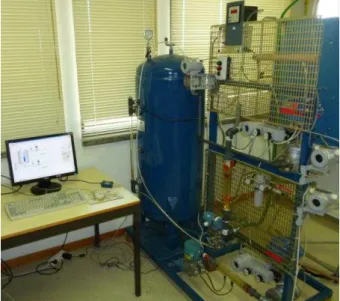
2. PHYSICAL PROCESS

The physical process was built to train undergraduate students in the principles of process control and FF instrumentation. The process contains all the equipment needed to run the following control loops (see figures 3 and 4):

 Level control loop: The water level inside the closed tank is measured by the transmitter LT1 and is controlled by operating the control valve FCV1. Information about water inflow, water temperature at the bottom of the tank, and air pressure at the top of the tank is provided by transmitters FT1, TT1 and PT1, respectively. The tank is equipped with an exhaust valve to prevent pressures above 3 bar.

 Flow control loop: The flow of water leaving the tank is measured by the transmitter FT2 and is controlled by operating the control valve FCV2.

The level control loop can be replaced by a pressure control loop by considering the signal from transmitter PT1 as the process variable. This was not the case in the current study.

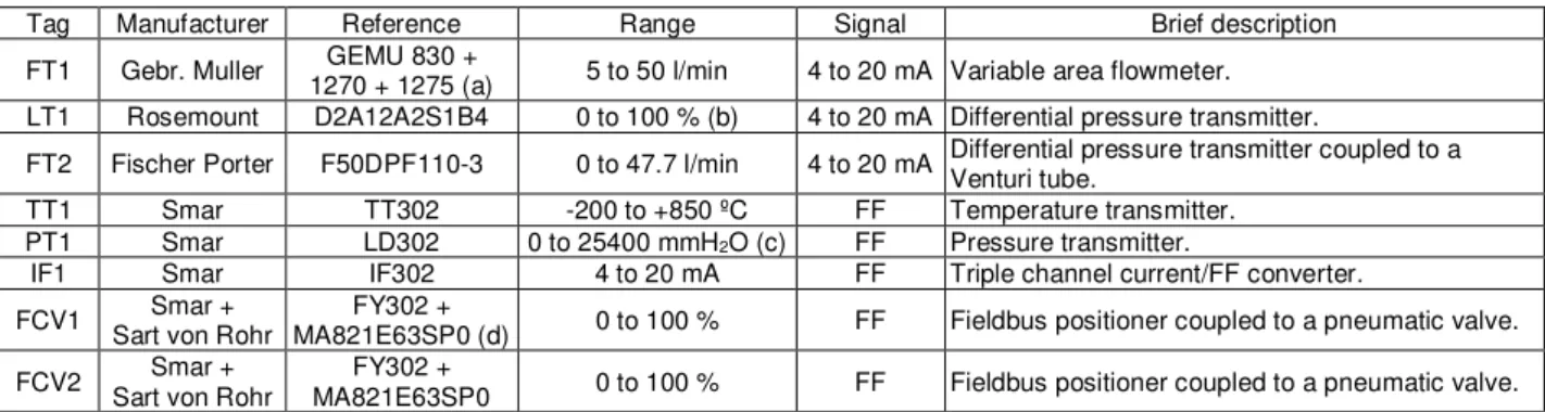
Table 1 summarizes the main characteristics of the

instruments installed on the physical process. The interface with analog transmitters (FT1, LT1 and FT2) was done using IF1, a triple channel current/FF converter. All converters, transmitters and control valves were properly verified and calibrated before experiments took place.

FF instruments were tied in a single H1 segment

powered with 24 VDC and terminated by a 100 Ω

resistor in series with a 100 nF capacitor. The H1 bus was connected directly to a computer (overcoming the H2 level) by means of an interface board that acts as linking device (model USB-8486 from National Instruments (NI) [7]). Finally, on the computer, it was installed all the software needed to configure and supervise the pilot plant, namely NI-FBUS Configurator version 4.0.1, and LabVIEW version 2009 SP1 plus Datalogging and Supervisory Control (DSC) module.

Fig. 3 – Picture of the physical process.

Fig. 4 – P&I diagram of the physical process. LT1

FT2

V-1 FCV1

AI

AO

IF1-2

PID PV

Set-point (level)

AI AO

IF1-3

PID FCV2

PV

Set-point (flow)

V-2 FT1

AI IF1-1

Outgoing water Incoming

water

Closed tank 240 liters AI

PT1

(5)

3. CONFIGURATION OF FF

INSTRUMENTS

The configuration of FF instruments is very challenging because it takes into account the dynamics of the physical process and the multitude of options offered by functional blocks. The only way to deal with this level of complexity is by using powerful software configuration tools, as is the case of NI-FBUS Configurator [8].

The configuration was done online having all FF instruments powered up and remotely visible. This requires patience (because the H1 bus is slow) but gives the chance to fix errors incrementally. The job was done instrument by instrument walking through the following steps:

1. The instrument was reset to its factory defaults. 2. A unique address from 17 to 247 was assigned to

the instrument (address 16 is automatically reserved by the interface board). This range is indicated for permanent instruments.

3. One or more FBs were instantiated to provide processing power for the instrument (according application needs).

4. Unique tags were assigned to the instrument and its functional blocks.

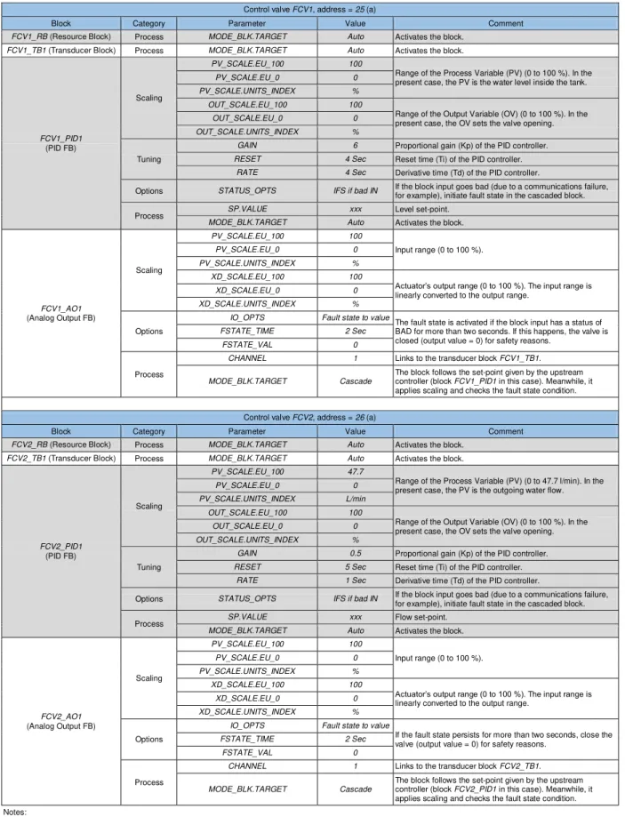
5. Each functional block was configured by editing its parameters according the desired behavior (see table 2). For this purpose it was essential to study the meaning of each parameter and the options it offers [9]. Helpful information was found in the operation manuals of the instruments [10-13].

The interface board was configured as the primary master by resetting all its parameters to the default values. No other (redundant) masters were implemented.

Having configured the H1 bus, it was time to build

a control application for the pilot plant. The application, shown in figure 5, is composed by three main sections:

1. The top section instructs the instruments TT1, PT1 and IF1 (channel 1) to log their input values and pass them to the interface board. The log has a fixed capacity of 15 values. This data is non-critical, has low priority, and is passed through unprogrammed dialogues.

2. The middle section implements the level loop control. The loop is closed by a PID controller that receives the process variable from the level transmitter LT1 (via channel 2 of the converter IF1), and writes the output variable to the positioner of the control valve FCV1. The AO function block feeds back its state to increase the loop consistency: if the AO function block breaks the loop (by passing to Manual mode, for example) the controller stops working and follows the valve opening; if the loop is restored the controller resumes its operation automatically. 3. The bottom section is similar to the middle one,

with the difference that it applies to the flow control loop. The process variable comes from the flow transmitter FT2 (via channel 3 of converter IF1), and the output variable goes to the positioner of the control valve FCV2.

The schedule of the control application is shown in figure 6. The configurator gives time for instruments to do internal processing (blue bars), as well as to exchange data across the H1 bus (red bars). The flow control loop has a period of 400 ms, while the (slower) level control loop allows a more

“relaxed” period of about 800 ms.

Table 1. Field instruments.

Tag Manufacturer Reference Range Signal Brief description

FT1 Gebr. Muller GEMU 830 +

1270 + 1275 (a) 5 to 50 l/min 4 to 20 mA Variable area flowmeter. LT1 Rosemount D2A12A2S1B4 0 to 100 % (b) 4 to 20 mA Differential pressure transmitter.

FT2 Fischer Porter F50DPF110-3 0 to 47.7 l/min 4 to 20 mA Differential pressure transmitter coupled to a Venturi tube.

TT1 Smar TT302 -200 to +850 ºC FF Temperature transmitter. PT1 Smar LD302 0 to 25400 mmH2O (c) FF Pressure transmitter.

IF1 Smar IF302 4 to 20 mA FF Triple channel current/FF converter.

FCV1 Smar + Sart von Rohr

FY302 +

MA821E63SP0 (d) 0 to 100 % FF Fieldbus positioner coupled to a pneumatic valve.

FCV2 Smar + Sart von Rohr

FY302 +

MA821E63SP0 0 to 100 % FF Fieldbus positioner coupled to a pneumatic valve. Notes:

a) GEMU 830 refers to the variable area flowmeter, GEMU 1270 refers to the displacement/voltage converter, and GEMU 1275 refers to the voltage/current converter with local indicator.

b) The range in meters depends on the dimensions of the tank. c) Gauge pressure.

(6)

Table 2. Configuration of FF instruments.

Temperature transmitter TT1, address = 20 (a)

Block Category Parameter Value Comment

TT1_RB (Resource Block) Process MODE_BLK.TARGET Auto Activates the block.

TT1_TB1 (Transducer Block)

I/O Config SENSOR_CONNECTION Three wires A three-wire PT100 IEC was used as the primary sensor.

Others TWO_WIRES_COMPENSATION Disable The three-wire connection compensates cable resistance.

SENSOR_TRANSDUCER_NUM 1 Sensor index.

Process MODE_BLK.TARGET Auto Activates the block.

TT1_TB2 Transducer Block) Others SENSOR_TRANSDUCER_NUM 2 Sensor index.

TT1_AI1

(Analog Input FB)

Scaling L_TYPE Direct Values from the transducer block are used directly (in ºC).

Trends OUT Trend  Enables trending for parameter OUT.

Process CHANNEL 1 Links to the transducer block TT1_TB1.

MODE_BLK.TARGET Auto Activates the block.

Pressure transmitter PT1, address = 21 (a)

PT1_RB (Resource Block) Process MODE_BLK.TARGET Auto Activates the block.

PT1_TB1 (Transducer Block) Process MODE_BLK.TARGET Auto Activates the block.

PT1_AI1

(Analog Input FB)

Scaling

XD_SCALE.EU_100 25400

Transducer’s input range (between 0 and 25400 mmH2O.

XD_SCALE.EU_0 0 XD_SCALE.UNITS_INDEX mmH2O (68ºF)

OUT_SCALE.EU_100 36.1263

Output range (between 0 and 36.1263 psig).

OUT_SCALE.EU_0 0 OUT_SCALE.UNITS_INDEX psig

L_TYPE Indirect The input range is linearly converted to the output range (in psig).

Process CHANNEL 1 Links to the transducer block PT2_TB1.

Current to FF converter IF1, address = 23 (a)

IF1_RB (Resource block) Process MODE_BLK.TARGET Auto Activates the block.

IF1_TB1 (Transducer Block) Process MODE_BLK.TARGET Auto Activates the block.

IF1_AI1

(Analog Input FB)

Scaling

XD_SCALE.EU_100 20

Transducer’s input range (4 to 20 mA).

XD_SCALE.EU_0 4 XD_SCALE.UNITS_INDEX mA

OUT_SCALE.EU_100 50

Output range (0 to 50 l/min). This range applies to the incoming water flow.

OUT_SCALE.EU_0 0 OUT_SCALE.UNITS_INDEX L/min

L_TYPE Indirect The input range is linearly converted to the output range.

Process CHANNEL 1 Links to the transducer block IF1_TB1.

IF1_AI2

(Analog Input FB)

Scaling

OUT_SCALE.EU_100 100

Output range (0 to 100 %). This range applies to the water level inside the tank.

OUT_SCALE.EU_0 0 OUT_SCALE.UNITS_INDEX %

L_TYPE Indirect The input range is linearly converted to the output range.

IF1_AI3

(Analog Input FB)

Scaling

OUT_SCALE.EU_100 47.7

Output range (0 to 47.7 l/min). This range applies to the outgoing water flow.

OUT_SCALE.EU_0 0 OUT_SCALE.UNITS_INDEX L/min

L_TYPE Indirect Sq Root

The input range is converted to the output range by applying the square root operation. Useful for flow meters based on differential pressure.

(7)

Table 2 (continued) Configuration of FF instruments.

Control valve FCV1, address = 25 (a)

FCV1_RB (Resource Block) Process MODE_BLK.TARGET Auto Activates the block.

FCV1_TB1 (Transducer Block) Process MODE_BLK.TARGET Auto Activates the block.

FCV1_PID1

(PID FB)

Scaling

PV_SCALE.EU_100 100

Range of the Process Variable (PV) (0 to 100 %). In the present case, the PV is the water level inside the tank.

PV_SCALE.EU_0 0 PV_SCALE.UNITS_INDEX % OUT_SCALE.EU_100 100

Range of the Output Variable (OV) (0 to 100 %). In the present case, the OV sets the valve opening.

Tuning

GAIN 6 Proportional gain (Kp) of the PID controller.

RESET 4 Sec Reset time (Ti) of the PID controller.

RATE 4 Sec Derivative time (Td) of the PID controller.

Options STATUS_OPTS IFS if bad IN If the block input goes bad (due to a communications failure,

for example), initiate fault state in the cascaded block.

Process SP.VALUE xxx Level set-point.

FCV1_AO1

(Analog Output FB)

Scaling

PV_SCALE.EU_100 100

Input range (0 to 100 %).

PV_SCALE.EU_0 0 PV_SCALE.UNITS_INDEX % XD_SCALE.EU_100 100

Actuator’s output range (0 to 100 %). The input range is

linearly converted to the output range.

XD_SCALE.EU_0 0 XD_SCALE.UNITS_INDEX %

Options

IO_OPTS Fault state to value _{The fault state is activated if the block input has a status of}

BAD for more than two seconds. If this happens, the valve is closed (output value = 0) for safety reasons.

FSTATE_TIME 2 Sec

FSTATE_VAL 0

Process

CHANNEL 1 Links to the transducer block FCV1_TB1.

MODE_BLK.TARGET Cascade

The block follows the set-point given by the upstream controller (block FCV1_PID1 in this case). Meanwhile, it applies scaling and checks the fault state condition.

Control valve FCV2, address = 26 (a)

FCV2_RB (Resource Block) Process MODE_BLK.TARGET Auto Activates the block.

FCV2_TB1 (Transducer Block) Process MODE_BLK.TARGET Auto Activates the block.

FCV2_PID1

(PID FB)

Scaling

PV_SCALE.EU_100 47.7

Range of the Process Variable (PV) (0 to 47.7 l/min). In the present case, the PV is the outgoing water flow.

PV_SCALE.EU_0 0 PV_SCALE.UNITS_INDEX L/min

OUT_SCALE.EU_100 100

Range of the Output Variable (OV) (0 to 100 %). In the present case, the OV sets the valve opening.

Tuning

GAIN 0.5 Proportional gain (Kp) of the PID controller.

RESET 5 Sec Reset time (Ti) of the PID controller.

RATE 1 Sec Derivative time (Td) of the PID controller.

Options STATUS_OPTS IFS if bad IN If the block input goes bad (due to a communications failure, _{for example), initiate fault state in the cascaded block.}

Process SP.VALUE xxx Flow set-point.

FCV2_AO1

(Analog Output FB)

Scaling

PV_SCALE.EU_100 100

Input range (0 to 100 %).

PV_SCALE.EU_0 0 PV_SCALE.UNITS_INDEX % XD_SCALE.EU_100 100

Actuator’s output range (0 to 100 %). The input range is

linearly converted to the output range.

XD_SCALE.EU_0 0 XD_SCALE.UNITS_INDEX %

Options

IO_OPTS Fault state to value

If the fault state persists for more than two seconds, close the valve (output value = 0) for safety reasons.

FSTATE_TIME 2 Sec

FSTATE_VAL 0

Process

CHANNEL 1 Links to the transducer block FCV2_TB1.

MODE_BLK.TARGET Cascade

The block follows the set-point given by the upstream controller (block FCV2_PID1 in this case). Meanwhile, it applies scaling and checks the fault state condition. Notes:

(8)

Fig. 5 – Control application.

Fig. 6 – Schedule of the control application.

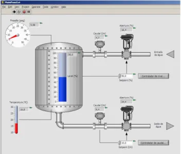
4. SUPERVISION SOFTWARE

The supervision software allows the pilot plant to be operated by people that are not experts on the FF technology. It hides low level configuration details and exposes system variables as numeric quantities.

The supervision software was developed in LabVIEW using the facilities provided by the DSC module [14]. The communication with FF infrastructure was done using the OPC-DA (Open Process Control Data Access) server [15-16] that comes with the NI-FBUS Configurator. The development went through the following stages:

1. An OPC client was created and connected to the OPC-DA server. The server exposes data items representing the parameters of all online functional blocks.

2. The data items of interest (those related with IN, OUT, SP, tuning and state parameters) were bound to shared variables created expressly for that purpose.

3. Each shared variable was configured in terms of

data type, access type (read only or read/write), alarming (HiHi, Hi, Lo and LoLo alarms), update dead band, alarm and data logging, and security (remote access permissions).

4. A virtual instrument was built to provide a rich graphical interface for the operator (see figure 7). The controls and indicators were bound to the shared variables to make the front panel synchronized with the system. The operator can read process variables, adjust set-points and tune controllers. No alarm support was implemented (that was left to future work).

It should be noted that stages 1, 2 and 3 were done following the procedures described in [17].

Fig. 7 – Supervision program.

5. EXPERIMENTAL RESULTS

Both control loops were tested over their dynamic ranges. For each controller, the set-point, process and output variables were remotely monitored and recorded. The experiments were carried out according the following methodology:

1. The PID controllers were tuned in advance using the trial and error method. The level controller was configured with proportional gain Kp = 6, reset time Ti = 4 s and derivative time Td = 4 s. The flow controller was configured with Kp = 0.5, Ti = 5 s and Td = 1 s.

2. The system was started with level and flow set-points of 50 % and 10 l/min, respectively. Time was given for all variables to stabilize.

3. Data recording was started at t = 0 min.

4. At t = 1 min the level set-point was changed to 80 %.

(9)

6. At t = 14 min the level set-point returned to 50 %. 7. At t = 18 min the flow set-point was changed to

15 l/min.

8. At t = 21 min the flow set-point was changed to 5 l/min.

9. At t = 24 min the flow set-point returned to 10 l/min.

10.Data recording was stopped at t = 28 min.

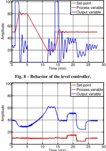
Regarding the level control loop (see figure 8), the collected data can be analyzed as follows:

 At t = 1 min and t = 14 min the controller opens valve FCV1 to increase the level. The process response has a small overshoot and stabilizes after 1 min (approximately).

 At t = 5 min the controller closes valve FCV1 to decrease the level. The process response has negligible overshoot and stabilizes almost immediately.

 The level controller is insensitive to flow variations due to the large capacity of the tank.

 The level controller is characterized by good tracking capability, small overshoot, short settling time, and good immunity to external disturbances (in particular those related with flow variations). Nevertheless, the oscillations observed in the output variable suggest that the controller should

be less “nervous” by reducing the gain or

increasing the reset time. The derivative time could also be increased to add more capacity of anticipation.

With respect to the flow control loop (see figure 9), the comments are similar:

 At t = 1 min and t = 14 min the flow has a slight increase (caused by the increment of the level) that is quickly canceled by the controller.

 From t = 5 min to t = 11 min the controller struggles to compensate the loss of flow caused by the continuous decline of the level.

 At t = 18 min and t = 24 the controller opens valve FCV2 to increase the flow. The process response has no overshoot and stabilizes after 1 min (approximately).

 At t = 21 min the controller closes valve FCV2 to decrease the flow. The process response has no overshoot and stabilizes after 1 min (approximately).

 The flow controller is characterized by good tracking capability, no overshoot, short settling time and good immunity to external disturbances (in particular those related with level variations).

The system was also tested in terms of safety by shutting down the LAS during a limited amount of time. With the system working normally, the interface board was disconnected from the bus and then reconnected one minute later. The response of the system was as follows:

 At the beginning the system seemed “frozen” with all variables retaining their value.

 Two seconds after (the value of parameter FSTATE_TIME) the control valves got into the fault state and closed their opening (FSTATE_VAL = 0). The tank was isolated from the exterior and the level and pressure on its interior were kept constant. Thus, thanks to the fault state mechanism implemented by AO function blocks, the system became safe.

 Two seconds after the reconnection (the value of parameter FSTATE_TIME) the control valves got out of the fault state and the system resumed its normal operation. This demonstrates that the H1 bus has self-recovery capability.

During all experimental tests the supervision software worked as expected demonstrating good robustness, performance and ergonomics.

Fig. 8 – Behavior of the level controller.

Fig. 9 – Behavior of the flow controller.

0 5 10 15 20 25 30

0 20 40 60 80 100

Time (min)

A

m

p

litu

d

e

Set-point Process variable Output variable

0 5 10 15 20 25 30

0 20 40 60 80 100

Time (min)

A

m

p

litu

d

e

(10)

6. CONCLUSION

The main topics of the FF technology were presented and a real application was implemented on a pilot plant. Two different control loops, involving level and flow, were tested to validate the safety mechanisms and the real-time capabilities of the FF system. The dynamic behavior of each control loop and the mutual effects caused by set-point changes were investigated. Everything worked as expected, with the system showing good performance even when large changes in set-points occurred.

7. REFERENCES

[1] Foundation Technical Specifications, Fieldbus Foundation, 1994-1998.

[2] David A. Glanzer, Foundation Fieldbus Technical Overview, Fieldbus Foundation, 2003.

[3] Ian Verhappen, Augusto Pereira, Foundation Fieldbus, 4th Edition, ISA - The International Society of Automation, 2012, ISBN 9781937560201.

[4] Kim R. Fowler, Electronic Instrument Design: architecture for the life cycle, Oxford University Press, 1996, ISBN 9780195083712.

[5] [Online] www.fieldbus.org

[6] Jonas Berge, Fieldbuses for Process Control: Engineering, Operation and Maintenance, ISA - The International Society of Automation, 2004, ISBN: 9781556179044.

[7] [Online]

http://sine.ni.com/nips/cds/view/p/lang/en/nid/207760

[8] [Online] www.natinst.com/fieldbus

[9] Function Blocks Instruction Manual, Smar, 2007. [10] TT302 - Fieldbus Temperature Transmitter - Operation and Maintenance Instructions Manual, Smar, 2011.

[12] LD302 - Fieldbus Pressure Transmitter - Operation and Maintenance Instructions Manual, Smar, 2012.

[12] IF302 - Triple Channel Current to Fieldbus Converter - Operation and Maintenance Instructions Manual, Smar, 2011.

[13] FY302 - Fieldbus Valve Positioner - Operation and Maintenance Instructions Manual, Smar, 2012. [14] [Online] www.ni.com/labview/labviewdsc [15] Jurgen Lange, Frank Iwanitz, Thomas J. Burke, OPC – From Data Access to Unified Architecture, 4th

Edition, Verlag GmbH, 2010, ISBN 9783800732425.

[16] OPC Data Access Specification version 3.00, OPC Foundation, 2003.

[17] LabVIEW Datalogging and Supervisory Control

Module Developer’s Manual, National Instruments, 2000.

Vítor Viegas was born in

Portugal in 1976. He received

his degree in Electrical

Engineering and Computer

Science from the Instituto

Superior Técnico (IST) of the

Universidade Técnica de

Lisboa (UTL) in 1999. After pursuing studies, he received the MSc and PhD degrees from the same school in 2003 and 2012, respectively. He works as Assistant Professor at the Instituto Politécnico de Setúbal (IPS). His main research activities concern smart transducers, fieldbus/distributed control systems, and industrial informatics.

J. M. Dias Pereira (M’00 -

SM’04) was born in Portugal in 1959. He received his degree in Electrical Engineering from the Instituto Superior Técnico (IST) of the Universidade Técnica de Lisboa (UTL) in 1982. During almost eight years he worked for Portugal Telecom in digital

switching and transmission

systems. In 1992, he returned

to teaching as Assistant