www.hydrol-earth-syst-sci.net/10/245/2006/ © Author(s) 2006. This work is licensed under a Creative Commons License.
Earth System
Sciences
Distributed hydrological modelling of total dissolved
phosphorus transport in an agricultural landscape,
part I: distributed runoff generation
P. G´erard-Marchant1, W. D. Hively2, and T. S. Steenhuis1
1Department of Biological and Environmental Engineering, Cornell University, Ithaca, NY 14853, USA 2Department of Natural Resources, Cornell University, Ithaca, NY 14853, USA
Received: 30 June 2005 – Published in Hydrol. Earth Syst. Sci. Discuss.: 22 August 2005 Revised: 30 November 2005 – Accepted: 21 February 2006 – Published: 26 April 2006
Abstract. Successful implementation of best management practices for reducing non-point source (NPS) pollution re-quires knowledge of the location of saturated areas that pro-duce runoff. A physically-based, fully-distributed, GIS-integrated model, the Soil Moisture Distribution and Rout-ing (SMDR) model was developed to simulate the hydrologic behavior of small rural upland watersheds with shallow soils and steep to moderate slopes. The model assumes that grav-ity is the only driving force of water and that most overland flow occurs as saturation excess. The model uses available soil and climatic data, and requires little calibration.
The SMDR model was used to simulate runoff produc-tion on a 164-ha farm watershed in Delaware County, New York, in the headwaters of New York City water supply. Apart from land use, distributed input parameters were de-rived from readily available data. Simulated hydrographs compared reasonably with observed flows at the watershed outlet over a eight year simulation period, and peak timing and intensities were well reproduced. Using off-site weather input data produced occasional missed event peaks. Sim-ulated soil moisture distribution agreed well with observed hydrological features and followed the same spatial trend as observed soil moisture contents sampled on four transects. Model accuracy improved when input variables were cali-brated within the range of SSURGO-available parameters. The model will be a useful planning tool for reducing NPS pollution from farms in landscapes similar to the Northeast-ern US.
Correspondence to:T. S. Steenhuis ([email protected])
1 Introduction
Reducing agricultural non-point source (NPS) pollution has become a focus for watershed management programs that maintain and improve water quality. Significant NPS pollu-tion originates from hydrologically active areas where runoff is generated, and that also have high soil nutrient concentra-tions (Gburek et al., 1996). Successful implementation of best management practices for reducing NPS pollution re-quires the knowledge of the location of frequently-saturated areas prone to overland flow generation, termed hydrologi-cally sensitive areas (HSAs) (Walter et al., 2000).
Overland flow generation can occur by two mechanisms. Infiltration-excess runoff (also called Hortonian overland flow) takes place when precipitation rate exceeds soil infiltra-tion capacity (Horton, 1933, 1940). This mechanism is pre-dominant on low organic matter arid and semiarid soils that are prone to crusting and on compacted areas during high-intensity rainfall events. In contrast, saturation-excess over-land flow occurs when precipitation falls on saturated soil. Location of saturation-excess overland flow generation does not depend on rainfall intensity but on topography, soil prop-erties, and local hydrological conditions, such as high water table (Hewlett and Hibbert, 1967; Dunne and Black, 1970; Hewlett and Nutter, 1970; Dunne et al., 1975; Beven and Kirby, 1979).
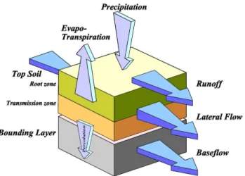
Fig. 1. Schematic representation of the water balance components over one cell.
et al., 1997; Srinivasan et al., 1998) or GWLF (Haith and Shoemaker, 1987; Haith et al., 1992; Schneidermannet al., 2002) are usually based on Hortonian overland flow genera-tion mechanisms. With these models, topographical informa-tion is not an important predictor of total runoff and nutrient loads to the streams. However, when overland flow is gen-erated by saturation- excess mechanisms, landscape position is a determining factor, and the temporal distribution of vari-able source areas must be estimated. Therefore, only models that preserve the spatial information during the simulation can accurately simulate saturation-excess overland flow.
Typical fully-distributed spatial models include the Syst`eme Hydrologic Europ´een, SHE (Abbott et al., 1986a, b; Refsgaard and Storm, 1995); TOPMODEL (Beven, 1997; Beven and Kirkby, 1979; Saulnieret al., 1998); Distributed Hydrology Soil Vegetation Model, DHSVM (Wigmosta et al., 1994; Wigmosta et al., 2002; Wigmosta and Perkins, 2001) and the Soil Moisture Distribution and Routing model, SMDR. The SMDR model is based on a soil moisture bal-ance calculation initially developed by Steenhuis and van der Molen (1986), later modified and integrated into the Geographic Resources Analysis Support System (GRASS) Geographic Information System (GIS) (US Army C.E.R.L., 1991; Neteler and Mitasova, 2002) by Zollweg et al. (1996), Frankenberger et al. (1999) and Kuo et al. (1999). This model is currently maintained by the Soil and Water Labora-tory, Cornell University (Soil and Water LaboraLabora-tory, 2003). SMDR was specifically designed for application on small ru-ral watersheds of the Northeastern United States, character-ized by soils overlying slowly permeable layers at shallow depths and moderate to steep slopes. It differs from other models such as SHE or DHVSM in that it uses only readily available input data. Unlike TOPMODEL, it does not assume a water table underlying the whole watershed, but uses soil data on depth to restrictive layer to determine the lower soil boundary.
In the recent years, SMDR has been successfully ap-plied to predict discharge data in several watersheds of the Catskills Mountain region, New York (Frankenberger et al., 1999; Mehta et al., 2004), in Central New York (Kuo et al., 1999; Johnson et al., 2003), and in Pennsylvania (Srini-vasanet al., 2005). Validation of the model distributed out-puts has been limited due to the difficulty of collecting accu-rate distributed data.
The objective of this paper is, therefore, to validate SDMR integrated (i.e. runoff at the watershed outlet) and distributed results. The study watershed is a 164-ha dairy farm, located in the northern Catskills region of Delaware County, NY, within the headwaters of Cannonsville reservoir, the third largest reservoir of the New York City water supply system. Streamflows and streamwater nutrient concentrations have been measured at the watershed outlet since 1993 (Bishop et al., 2003, 2005). Detailed management records are also available, and this farm provides an ideal context for appli-cation of the model and verifiappli-cation of results.
2 Description of the SMDR model
The purpose of SMDR is to identify the location and evo-lution of variable source areas for overland flow generation and to estimate water fluxes to streams and groundwater. The SMDR is intended as a tool for planners or groups interested in watershed management. Therefore, it does not require ex-tensive calibration and is designed to use data that are read-ily available in electronic form: (i) a digital elevation map, (ii) a soil type map and the associated table of soil hydro-logic properties, (iii) a land use and land cover map, and (iv) weather data (temperature, precipitation and potential evap-otranspiration). Details of input data requirements are given in a following section.
Use of SMDR is limited to upland, well-vegetated water-sheds, where soils have a high infiltration capacity and slopes over 3%. In many cases, a low permeability layer, such as bedrock or fragipan, is present at a relatively shallow depth. Watersheds of this type occur not only in the Northeastern United States, but also in many other parts of the world.
The SMDR divides the watershed in square gridcells, with typical cell dimensions ranging from 5 to 30 m. Larger di-mensions tend to misrepresent the landscape curvatures and lead to unreasonably high estimates of soil water content (Kuo et al., 1999). In practice, the minimum grid size de-pends on the resolution of the DEM. Within each cell, soil properties are assumed to be homogeneous. Soil horizons above the low-conductivity restricting layer are grouped into a single surface soil layer. This surface soil layer is then decomposed into two functional sublayers, corresponding to the rooting zone and a transmission zone.
computational speed, accuracy of results, and data availabil-ity. Daily water inputs to the top soil layer of each cell are daily precipitation and lateral flow from surrounding ups-lope cells. Outputs are lateral flow to surrounding downsups-lope cells, percolation through the restrictive layer, and evapotran-spiration. A schematic representation of the water balance is illustrated Fig. 1. The water mass balance equation can be expressed for each cell as:
zW2|θ (t )−θ (t−1t )| = |RF (t )+SM(t )|
+ Qi(t )−Qo(t )
− ET (t )−P (t )−SE(t )
(1)
where z is the thickness of the surface soil (m), W the (square) grid size (m), θ the cell average water content (cm3.cm−3),1t the time step (d),RF andSM the rainfall and snowmelt volumes, respectively,Qi the volume of
wa-ter received through lawa-teral flow from surrounding upslope cells,Qothe volume of water lost through lateral flow to
sur-rounding downslope cells,ET the volume of water lost by evapotranspiration,P the volume of water lost by percola-tion through the bounding layer, andSEthe saturation excess runoff. Volumes are expressed in (m3). Although the mass balance components are tightly coupled, they are estimated separately for computational simplicity. They are presented hereafter in the order in which they are calculated for each time step.
2.1 Precipitation
Daily precipitation is first partitioned into rain or snow, de-pending on the observed daily mean air temperature (◦C), corrected as necessary for local elevation by the adiabatic lapse rate of 6.5×10⁻³C.m−1 (Boll et al., 1998). Rain-fall RF is identified with precipitation on cells where air temperature is greater than −1◦C. Snowmelt SM is
com-puted following a simple land-cover dependent temperature index method (US Army Corps of Engineers, 1960). Rainfall and snowmelt occurring on impervious areas, e.g. roads and buildings, are converted directly to overland flow.
2.2 Moisture redistribution
Water inputs are assumed to infiltrate and are added to the water already stored in the surface layer. After infiltration, three characteristic moistureθf, θm andθs are considered,
corresponding to field capacity, macroporous drainage limit and saturation, respectively. Field capacity is defined as the moisture content below which no drainage takes place. The macroporous drainage limit corresponds to the minimum wa-ter content required to activate macropore flows, and is re-lated to the depth to the slowly permeable layer: the shal-lower the slowly permeable layer, the larger the drainage limit (Boll et al., 1998). The moisture content at saturation is identified with effective porosity (i.e. porosity corrected by rock fragment and organic matter content).
When the average soil water content θ¯ is less than the macroporous drainage limit, the moisture profile is assumed uniform throughout the top layer of soil. Otherwise, a sat-urated layer of thickness zs is formed, with average water
contentθ, so that
zθ =(z−zs)θm+zsθs (2)
2.3 Lateral flows
Lateral outflows are calculated by integrating Darcy’s law over soil depth, grid width and time step. After identify-ing the hydraulic gradient with the local surface slope σ
(m.m−1), and assuming that the hydraulic conductivity does not vary significantly with position or time during one time step, it comes eventually:
Qo= −κ K(θ ) z W σ 1t (3)
where K is the average hydraulic conductivity of the layer (m.day−1),κ a depth-dependent multiplier (typical range of 2 to 10) introduced to correct transmissivities for preferen-tial flows in macropores (Boll et al., 1998). The average hy-draulic conductivityKis defined as:
K(θ )=0 for θ < θf
K(θ )=Ks exp
h
−αθs−θ
θs−θf i
for θf ≤θ < θm
K(θ )=Km + Ks θθ−θm
s−θm for θm≤θ
(4)
whereKs=K(θs)andKm=K(θm)are the hydraulic
conduc-tivity at saturation and at macroporous drainage limit, respec-tively, andαis an universal constant equal to 13 for a large range of soils (Bresler et al., 1978; Steenhuis and van der Molen, 1986).
Lateral outflows from each cell are then distributed ac-cording to local aspect between one cardinal and one diag-onal downslope neighboring cells, following theD∞
algo-rithm (Tarboton, 1997). On each cell, the lateral inflowQi
is defined as the sum of the contributions received from the upslope surrounding cells.
2.4 Evapotranspiration
EvapotranspirationET is calculated by solving the differen-tial equation:
zr
dθ
dt = −Kc E (5)
where zr is the depth of the rooting zone (m), Kc a basal
evapotranspiration coefficient introduced to reflect differ-ences among vegetation types (−) (Allen et al., 1998), and
rate, Eref, when soil moisture exceeds a given “evapotran-spiration limit” θl, usually set to field capacity. The
po-tential evapotranspiration rateEref is calculated daily from
temperature data, following the Hargreaves and Samani’s (1985) method or a simplified Priestley and Taylor (1972) method. Rooting depthszr and basal coefficientsKcare
cal-culated for each vegetative cover, depending on its develop-ment stage. Vegetative developdevelop-ment is calculated as a func-tion of cumulative growing degree-days, i.e. the cumulative difference of daily average temperatures and a vegetation-type dependent basal temperatureTb(◦C). Five development
stages are defined, according to cumulative growing degree-day thresholds and a final winter cutoff condition (Jensen et al., 1990). Growing degree-days accumulation starts when average daily air temperature is larger than the basal temper-atureTbfor five consecutive days (Goudriaan and van Laar,
1994). Data for the basal coefficients and growing-degree day threshold are compiled from literature or estimated from local records.
2.5 Percolation
Percolation of water through the fractures and cracks in the bedrock and, to a lesser extent, through the dense fragipan (Soren, 1963), is computed for each cell as:
P = min[K(θ );Ksub]W21t (6)
whereKsubis the conductivity at saturation of the cell sub-stratum, (m.day−1), and where the hydraulic conductivityK
is given by Eq. (4). Percolation stops when the average water content of the bottom structural layer is less than field capac-ity.
Identification of percolation pathways requires some knowledge of the geometry of the fractures. Unfortunately, such data are scarce. Therefore, it is assumed that at each time step, only a fractionr of the total percolating volume flows to the streams, with the remainder lost to regional flow. Percolation to the stream constitutes the stream baseflowBF
(m3), such as
BF =rX
i
Pi (7)
wherePiis the percolation volume simulated on cell (i) (m3),
and where the summation domain is the entire watershed. Conceptually, this does not mean that a drop of water that percolates in the substratum becomes immediately baseflow. Water, as in previous versions of the model, enters into a sub-surface reservoir. In the current implementation, the reser-voir volume is fixed so that for each quantity of water that enters the reservoir, a similar quantity becomes baseflow. Al-though for the water balance the distinction of what water enters the stream as baseflow is immaterial, it becomes im-portant when nutrient transport is considered.
2.6 Overland flow and streamflow generation
At the end of each time step, any water in excess of saturation becomes saturation excess overland flowSE(m3). Overland flow is routed directly to the watershed outlet. Re-infiltration and interaction of overland flow with downslope soils are not considered.
3 Input data
Refsgaard and Strom (1996) stress that for a rigorous parametrization of hydrological systems, only the parame-ters that are pertinent to modeling and that can be directly measured or derived from field data should be selected. In SMDR, computation of the water balance requires, in ad-dition to climatic input, the knowledge of several parame-ters on each cell: z,θp,θl, θf,θm, θs, κ, Ks, zr, Kc, and
Ksub. Another parameter, the percolation coefficientr, has to be estimated on the watershed scale. To limit the risk of overparameterisation (Beven, 1996), parameters are actually grouped in generic classes reflecting only significant spatial variations. Typical classes consist of soil units, soil horizons, vegetative types and land covers. Parameter classes for the study watershed are defined in a following section.
3.1 Weather information
Daily minimum and maximum temperatures were obtained from a nearby weather station located at Delhi, New York, 438.9 m.s.l., (National Weather Service (USDC NOAA) co-operative observer station #302036, “Delhi 2 SE”), located about 20 km SW of the site (NCDC, 2000). Temperatures were corrected by −1.2◦C to account for the difference of elevation with the study watershed. Potential evapotranspira-tion ratesEref were calculated from daily temperature data,
following the Priestley and Taylor (1972) method. Precipi-tation was recorded at a 10-min interval, and integrated over one day. Onsite precipitation records were available from 1998 to 1999 only, for air temperatures greater than 1◦C.
When onsite information was not available, daily precipita-tion records from the Delhi weather staprecipita-tion were used in-stead. Daily stream flows were recorded on a 10-min basis by a gauge at the watershed outlet, and integrated over one day (Bishop et al., 2003).
3.2 Parameter classes 3.2.1 Topographic map
N
0 500
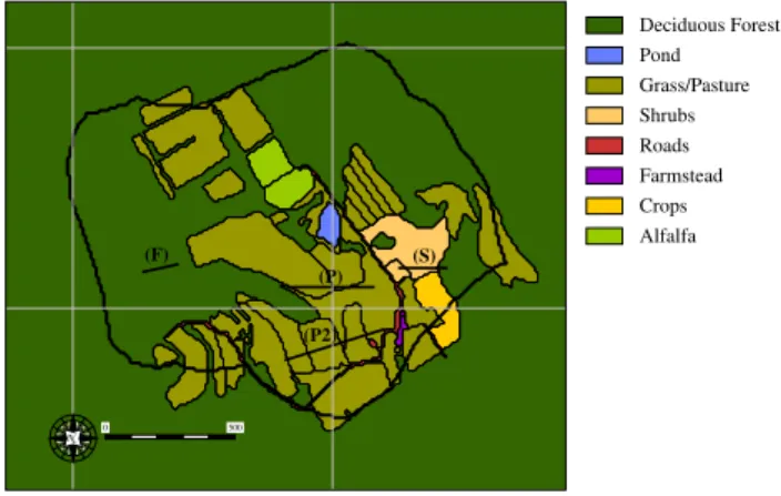
Fig. 2. Aerial photograph of the study watershed, with 5-m
eleva-tion contours (white lines). Solid black line: watershed boundary.
and to match the area above the streamflow monitoring sta-tion, and was finally verified by Hively (2004). An aerial photograph of the watershed, with 5-m elevation contours, is presented Fig. 2. Study watershed elevations range from 600 to 740 m.s.l. The main flow direction is oriented NNW-SSE. Slopes on the upper part of the watershed range from 2 to 40% (with an average about 17%), while slopes on the lower part range from 0 to 20% (with an average about 8%). 3.2.2 Soil type classes
Soil types and characteristics were derived from the SSURGO database (USDA-NRCS, 2000). The steeper, shal-lower (average thickness 65 cm) upper terrains are charac-terized by Halcott channery loams (loamy-skeletal, mixed, active, frigid Lithic Dystrudepts) and Vly channery silty loams (loamy-skeletal, mixed, superactive, frigid Typic Dys-trudepts). These terrains overlay a fractured horizontal bedrock. The flatter, deeper (average thickness 180 cm) lower terrains consist of moderately-well-drained Willowe-moc channery silt loams (coarse, loamy, mixed, frigid, Typic Fragiochrepts) and Onteora silt loams (coarse-loamy, mixed, semiactive, frigid Aquic Fragiudepts). These terrains are re-stricted by a dense fragipan. The watershed soil map is pre-sented in Fig. 3. No independent validation was carried out on the exact location of the boundaries between soil types. 3.2.3 Land covers and land uses
Because readily available MRLC land cover data were not sufficiently detailed for modeling at a 10-m gridcell reso-lution, a 1-m Chromatic InfraRed (CIR) digital
orthophoto-N
Ek,El: Elka−Vly complex Hc: Halcott, Mongaup and Vly soils TeB: Torull−Gretor complex Vl: Vly channery silt loam Water Fragipan limit Lh: Lewbeach channery loam Lk: Lewbeach & Lewbath soils No: Norchip silt loam Oe: Onteora channery silt loam Of: Onteora & Ontusia soils Wh: Willdin channery silt loam Wm: Willowemoc channery silt loam Wn: Willowemoc & Willdin soils
0 500
Fig. 3.SSURGO soil units map for the study watershed. Solid black
line: watershed boundary; dotted black line: fragipan-bedrock boundary
N
(P2) (P)
(S) (F)
Deciduous Forest Pond Grass/Pasture Shrubs Roads Farmstead Crops Alfalfa
0 500
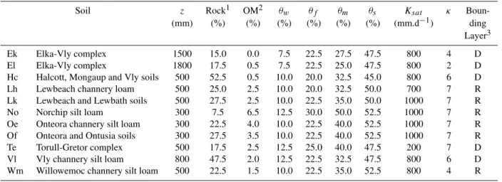
Fig. 4.Field boundaries, land uses for 2001 and sampling transects
location.
Table 1. Vegetation and land uses properties used in the calculation of evapotranspiration: rooting depthzr, basal evaportranspiration
coefficientKc, base temperatureTband growing degree thresholdsDD.
zr(mm) Kc Tb DDmax DD12 DD23 DD34
min max min max (◦C) (%) (%) (%)
Open Water 0 0 1.00 1.00 0 0 0 0 0
Roads/Buildings 0 0 1.00 1.00 0 0 0 0 0
Deciduous Forest 1500 1500 0.25 1.00 1 3500 0.10 0.15 0.93
Shrubland 750 750 0.20 1.00 1 2700 0.08 0.13 0.95
Grasslands/Herbaceous 600 600 0.20 1.00 1 4000 0.05 0.10 0.97
Row Crops 75 750 0.40 1.10 5 2100 0.15 0.40 0.90
Small Grains 75 750 0.40 1.10 5 2000 0.15 0.40 0.90
Fallow 600 600 0.20 1.00 3 3500 0.05 0.10 0.97
Alfalfa 1500 1500 0.20 1.20 1 4000 0.05 0.10 0.97
Grass/Hay + grazing 600 600 0.20 1.00 1 4000 0.05 0.10 0.97
Table 2.Soil characteristics for the study watershed.
Soil z Rock1 OM2 θw θf θm θs Ksat κ
Boun-(mm) (%) (%) (%) (%) (%) (%) (mm.d−1) ding Layer3
Ek Elka-Vly complex 1500 15.0 0.0 7.5 22.5 27.5 47.5 800 4 D
El Elka-Vly complex 1800 17.5 0.5 7.5 22.5 25.0 47.5 800 2 D
Hc Halcott, Mongaup and Vly soils 500 52.5 0.5 10.0 20.0 32.5 45.0 800 6 D Lh Lewbeach channery loam 500 25.0 2.5 10.0 20.0 32.5 50.0 700 7 R Lk Lewbeach and Lewbath soils 500 27.5 2.5 10.0 22.5 35.0 50.0 1000 7 R
No Norchip silt loam 300 7.5 6.5 12.5 30.0 50.0 52.5 1000 7 R
Oe Onteora channery silt loam 300 22.5 4.0 10.0 22.5 40.0 52.5 1000 7 R Of Onteora and Ontusia soils 300 27.5 3.5 10.0 22.5 40.0 52.5 1000 7 R Te Torull-Gretor complex 500 17.5 2.5 12.5 25.0 40.0 47.5 200 7 D Vl Vly channery silt loam 800 47.5 2.0 12.5 22.5 32.5 47.5 800 6 D Wm Willowemoc channery silt loam 500 22.5 1.5 10.0 22.5 35.0 52.5 800 4 R
1Rock and gravel content. 2Organic matter content.
3Bounding layer type – R: restricting (fragipan) – D : draining (bedrock).
3.3 Parameters definition 3.3.1 Vegetation properties
Minimum and maximum values of the basal evapotranspi-ration coefficientKc and the rooting depthzr were derived
from generic values reported in the literature (Jensen et al., 1990; Allenet al., 1998). For each vegetation type, growing degree-days thresholds and basal temperatures were adjusted prior to simulation, to reflect times of budding, leaf emer-gence and full canopy representative of the Central New York climate. Relevant information is reported in Table 1.
3.3.2 Directly available soil properties parameters
Jan. Feb. Mar. Apr. May Jun. Jul. Aug. Sep. Oct. Nov. Dec. 0 5 10 15 20 25 30 35 [10
-3 m 3 .m -2 .d -1 ] Observed Simulated
Jan. Feb. Mar. Apr. May Jun. Jul. Aug. Sep. Oct. Nov. Dec.
0 5 10 15 20 25 30 35 [10
-3 m 3 .m -2 .d -1 ] 0 5 10 15 20 25 30 35 Streamflows 1997
Jul. Aug. Sep. Oct. 0 0.2 0.4 0.6 0.8 1 50 40 30 20 10 0 Snowmelt 50 40 30 20 10 0 Precipitation [mm]
Jan. Feb. Mar. Apr. May Jun. Jul. Aug. Sep. Oct. Nov. Dec. 0 5 10 15 20 25 30 35 [10
-3 m 3 .m -2 .d -1 ] Observed Simulated
Jan. Feb. Mar. Apr. May Jun. Jul. Aug. Sep. Oct. Nov. Dec.
0 5 10 15 20 25 30 35 [10
-3 m 3 .m -2 .d -1 ] 0 5 10 15 20 25 30 35 Streamflows 1998
Jul. Aug. Sep. Oct. 0 0.2 0.4 0.6 0.8 1 50 40 30 20 10 0 Snowmelt 50 40 30 20 10 0 Precipitation [mm]
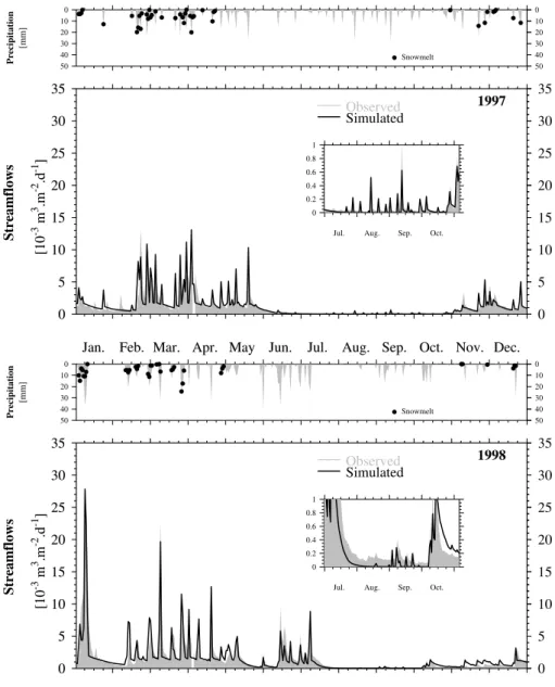
Fig. 5. (a)–(d)Comparison between observed (filled grey curve) and simulated (soild black line) hydrographs.
effect of macropores is based on the procedures by Boll et al. (1988) as described in Eq. (4). The selected properties values were then weighted by the structural layer thickness, averaged over the composite topsoil layer and rounded. Pa-rameters values for each soil type are presented in Table 2.
In previous versions of the model, the main soil sequence was decomposed as the superposition of several structural layers, as described by the SSURGO data base (Johnson et al., 2003; Metha et al., 2004). In the current version, the structural layers above the restricting layer (bedrock or fragi-pan) are aggregated into a composite surface soil layer, and soil depth zis defined as the sum depth of this composite layer.
Wilting point θp was calculated as the water content at
−1500 kPa, using SSURGO values of organic matter and clay contents, and a linear regression equation developed by Rawls and Brakensiek (1985). Field capacityθf was
calcu-lated as the sum ofθpand the midrange of SSURGO values
for available water content. Evapotranspiration limitθl was
set to field capacity.
3.3.3 Estimated soil properties parameters
Only four parameters are not readily available and have to be estimated: macroporous drainage limitθm, horizontal
Jan. Feb. Mar. Apr. May Jun. Jul. Aug. Sep. Oct. Nov. Dec. 0 5 10 15 20 25 30 35 [10
-3 m 3 .m -2 .d -1 ] Observed Simulated
Jan. Feb. Mar. Apr. May Jun. Jul. Aug. Sep. Oct. Nov. Dec.
0 5 10 15 20 25 30 35 [10
-3 m 3 .m -2 .d -1 ] 0 5 10 15 20 25 30 35 Streamflows 2000
Jul. Aug. Sep. Oct. 0 0.2 0.4 0.6 0.8 1 50 40 30 20 10 0 Snowmelt 50 40 30 20 10 0 Precipitation [mm]
Jan. Feb. Mar. Apr. May Jun. Jul. Aug. Sep. Oct. Nov. Dec. 0 5 10 15 20 25 30 35 [10
-3 m 3 .m -2 .d -1 ] Observed Simulated
Jan. Feb. Mar. Apr. May Jun. Jul. Aug. Sep. Oct. Nov. Dec.
0 5 10 15 20 25 30 35 [10
-3 m 3 .m -2 .d -1 ] 0 5 10 15 20 25 30 35 Streamflows 2001
Jul. Aug. Sep. Oct. 0 0.2 0.4 0.6 0.8 1 50 40 30 20 10 0 Snowmelt 50 40 30 20 10 0 Precipitation [mm]
Fig. 5.Continued.
saturation of the bounding layerKsub, and percolation frac-tion delivered to streamflow,r.
In previous versions of the model, decreasing values of the multipliersκ were allocated from the top structural layer to the bottom one (Mehta et al., 2004). In the current ver-sion, the multipliers were assumed to decrease exponentially with topsoil thickness, from 10 for the shallowest soils of the watershed to 2 for the deepest ones. The values were ini-tially chosen to reproduce field observations that hydraulic conductivities derived from bore hole measurements were up to one order of magnitude larger than those reported in the SSURGO database, for which conductivities are determined on disturbed samples (unpublished data).
The macroporous drainage limit, θm, is a key parameter
controlling subsurface lateral flows and percolation. Prelimi-nary investigations indicated that ifθmwas set to a low value,
simulated percolation would last for too long a period for wet soils, as compared with observed baseflows, and would restart after a too short period for dry soils, leading to over-estimated baseflows at the beginning and end of the summer period. Eventually, for soils with a restrictive layer of less than 3 m, the parameter was estimated from field capacity and soil depth, through the relation:
θm=θf|3/z|1/4 (8)
Table 3. Comparison of annual, summer and winter values of observed and simulated daily streamflows and efficiency criteria for the simulated period (1 January 1994–31 December 2001).
Year All 1994 1995 1996 1997 1998 1999 2000 2001
Annual
Precipitation (mm) 8577 1184 1047 1472 866 993 951 1230 834 Obs. Flows (mm) 4531 702 494 883 424 552 473 675 328 Simul. flows (mm) 4412 632 492 898 424 520 464 638 344 MNSa 0.661 0.632 0.638 0.604 0.769 0.746 0.635 0.413 0.579 MAEb 0.436 0.448 0.385 0.383 0.515 0.516 0.418 0.287 0.388 R2 0.584 0.571 0.465 0.625 0.581 0.752 0.673 0.483 0.496
Summer (1 May–31 October)
Precipitation (mm) 4422 611 588 776 367 515 480 604 480
Obs. Flows (mm) 1155 155 87 310 73 163 88 229 51
Sim. flows (mm) 1157 161 141 303 76 121 106 183 66 MNSa 0.656 0.568 0.505 0.757 0.903 0.733 0.336 0.182 −0.301 MAEb 0.473 0.390 0.271 0.513 0.760 0.573 0.354 0.212 0.065 R2 0.633 0.489 0.700 0.732 0.896 0.779 0.717 0.443 0.538
Winter (1 January–31 March, 1 November–31 December)
Precipitation (mm) 4155 573 459 696 499 478 471 625 354 Obs. Flows (mm) 3376 548 407 573 351 389 385 446 277 Sim. flows (mm) 3255 472 350 595 348 399 358 455 278 MNSa 0.506 0.526 0.257 0.457 0.439 0.707 0.407 0.444 0.531 MAEb 0.335 0.385 0.194 0.275 0.298 0.469 0.294 0.298 0.287 R2 0.539 0.535 0.357 0.586 0.427 0.737 0.664 0.465 0.440
aModified Nash Sutcliffe criterion (Chiew and McMahon, 1994).bMean Absolute Error (Ye et al., 1997).
water pressure – water content relationship is described by the Brooks and Corey (1964) model, and that field capacity is identified with the water content at a pressure of−30 kPa (equivalent to 3 m of water column). The exponent in Eq. (8) corresponds to a generic value of Brooks-Corey pore size dis-tribution index over a wide range of soils.
Following Frankenberger et al. (1999), a generic value of 1 mm·day−1 was assumed for the saturated conductiv-ity of fragipan layers, while a saturated conductivconductiv-ity of 2 mm·day−1was assumed for the slowly permeable bedrock layers. The percolation fractionr, was calibrated after sim-ulation to a value of 0.677, in order to match observed flows during a dry summer period (1997).
4 SMDR model integrated results
The SMDR model was applied to the study watershed over a 9-year period (1 January 1993 to 31 December 2001). The resulting hydrographs are presented in Figs. 5a–h. The first year of simulation (1993) is not shown as it was affected by the assumed initial water storage conditions. Outputs for each year were decomposed into two 6-month seasons, “summer” (May–October) and “winter” (November–April).
From 1993 to 2001, a total of 8577 mm of precipitation was recorded (4422 and 4155 mm for summer and winter
periods, respectively), and 4531 mm of streamflow was ob-served (1155 and 3376 mm for summer and winter periods, respectively). For the same period, simulated streamflow was 4412 mm (1157 and 3255 mm for summer and winter peri-ods, respectively). Precipitation and observed and simulated streamflows are reported for each simulated year in Table 3, along with the values of three efficiency criteria: modified Nash-Sutcliffe criterion MNS (Chiew and McMahon, 1994), mean absolute error MAE (Ye et al., 1997), and correlation coefficients R2. The MNS criterion is similar to the Nash-Sutcliffe criterion, but it uses square roots of flows instead of absolute flows. It is therefore more sensitive to low flow events than the classical Nash and Sutcliffe (1970) criterion. The mean absolute error characterizes how close the simu-lated results are from observations at each time step (Ye et al., 1997). The closer the value of any of the three criteria is to one, the better the simulation.
obtained for the dry summer 1997 on which the calibration of the percolation raterwas performed. This was expected since it was assumed, for lack of better data, that the fraction of the watershed contributing to percolation was constant. In reality it is not and because of the many springs in the water-shed, it could even be affected by the previous year’s rainfall. Therefore, more complex reservoir models requiring more parameters were also considered. However, they did not sig-nificantly improved baseflow simulations. It was finally de-cided to use the simplest model as presented above. Note that the lack of knowledge of the complicated underground flow paths is a limitation for any hydrology model applied to watersheds in the Catskills.
It is also of interest to evaluate the model’s performance by comparing the timing and intensities of simulated peak flows with observed data. Unlike watersheds where Horto-nian overland flow is the dominant process and where peak flows have a short duration (of a few minutes to a few hours), watershed where runoff is generated by saturation excess ex-hibit broader flow peaks. These peaks occur when a major portion of the watershed contributes to runoff, during peri-ods when total rainfall amounts exceeds evaporation greatly. Moreover, since precipitation data was available on a daily basis only, observed and simulated peak flows were com-pared at the same daily time step.
Peak flow timing, intensities and hydrograph recession were usually well simulated. Occasionally peaks were not re-produced in winter (e.g. 25 January 1996, 6 February 1997, 17 January 1998, 15 Feburary 2000 in Figs. 5c–g, respec-tively), while some peaks were incorrectly simulated during observed low winter flows (e.g. 23 January 1997, 22 March 1999 in Figs. 5d and f, respectively). This discrepancy was attributed to the use of off-site climate data, as described be-low.
Agreement between observed and simulated flows was better during summer (MNS=0.66, MAE=0.47, R2=0.63) than during winter (MNS=0.51, MAE=0.33, R2=0.54). Here again, peak timing and intensities were generally well pre-dicted, with a slight underestimation of peakflows. A signif-icant underestimation of peakflows was observed in August 2000 (Fig. 5g), when precipitation occurred late in the sea-son, as short-duration, high-intensity summer thunderstorms over dry soils. Low flows were usually underestimated (e.g. August 1998 and July 1999).
Three main sources can explain the occasional poor matches between observed and predicted hydrographs. First, water balance components are not perfectly mod-eled. Snowmelts are only crudely estimated by the temperatuindex method currently implemented. More re-alistic snowmelt routines involve calculation of a radiation balance, even simplified (Walteret al., 2005), but required data were not readily available. Soil freezing and interactions between rainfall and snow cover should also be taken into account. Moreover, infiltration-excess overland flow during summer months is modeled on impervious areas only and
not on other soils, which for high rainfall intensity summer storms will likely cause the underestimation of peakflows such as were observed in August 2000. Also, SMDR takes into account perched water tables only, and regional ground-water only indirectly. The latter is a direct consequence of the lack of information about the subsoil structure and the location of subsurface flow paths.
An additional source of errors comes from non-optimal pa-rameter calibration. For example, an overestimation of the soil drainage properties would lead to too rapid a depletion of the water storage by lateral flows, causing an underestima-tion of percolaunderestima-tion during summer months. This hypothesis can explain the simulation of lower summer flows than were observed.
Finally, weather data were obtained from an offsite station about 20 km from the site. In the summer, thunderstorms are localized, and precipitation measured at Delhi, NY may not equal precipitation occurring onsite. For example, on 7 August 2000, 18 mm of rain (as recorded in Delhi) produced only 0.7 mm of streamflow at the watershed outlet, while three days later, 15 mm of rain produced 7.3 mm of stream-flows. It is likely that the actual precipitation for the storm that hit Delhi on 7 August 2000 was in fact much less on the study watershed. Model results may improve substantially with the use of on-site climatic data. Similarly, the use of off-site temperature data may have contributed to the imper-fect reproduction of snowmelt events.
5 SMDR model distributed results
Alone, comparison of observed and simulated hydrographs is not a sufficient check of the distributed accuracy of hy-drological models. For example, Refsgaard and Knud-sen (1996) observed that after proper calibration, a con-ceptual lumped model (NAM) and a physically-based dis-tributed model (MIKE-SHE) predicted streamflows equally well. Similarly, Johnson et al. (2003) compared SMDR re-sults with outputs simulated by HSPF, an infiltration-excess based semi-distributed conceptual model. Both models gave equally accurate hydrographs despite their different runoff generation mechanisms (Johnson et al., 2003).
A classical approach to assess the efficiency of a dis-tributed model such as SMDR consists in the quantitative comparison of observed and simulated moisture contents at various locations throughout the watershed. Such a method is intrinsically limited by its local character, as samples are taken at specific locations, on particular dates. Even if this approach provides valuable information about the hydro-dynamic characteristics of the soils where the samples are taken, it usually fails to identify variable source areas on a larger scale and to capture their dynamics.
(Mehta et al., 2001, 2004), or indirect information about the position of hydrological features in the landscape. For exam-ple, diversion ditches and tile drains are usually installed to intercept overland flow and subsurface lateral flows, respec-tively, thus indicating the regular occurrence of runoff gener-ating areas upslope of these installations. In a related way, certain vegetation types, such as ferns and marsh grasses, grow preferentially in wet areas, and could be used as an indicator of the location of areas prone to generate runoff. Both direct and indirect validation approaches are presented below.
5.1 Transect sampling
Soil samples were collected at 10-m intervals along three transects on two occasions (8 June 2001 and 5 December 2001). The transects were chosen to represent various land uses and topography. A forested transect (“F”) was located on a steep hillslope, over bedrock-limited soils. Transect (“P”) was located on pasture fields, on gently sloping soils overlying a fragipan. Transect (“S”) was located on mod-erately steep shrubland. Sampling locations were identified by GPS for the eastern (“P”) and middle (“S”) transects, but could not be obtained the forested transect (“F”) because of the interference from tree canopy. The location of this latter transect was therefore only approximated from the DOQQ. Transect positions are plotted on the land use map in Fig. 4.
Single cores (48 cm3)were taken from each location at a depth from 2 to 6 cm. Each core was weighted and dried to determine gravimetric moisture content and soil bulk density. The samples were also sieved (2 mm) to correct the results for rock content. Soil moisture saturation degree was calcu-lated as:
2= mw
Vc−ms/ρs
(9) wheremw andms are the measured mass of water and dry
soil in the sample, Vc the core volume andρs the particle
density, after correction by the organic matter content. Rela-tive errors on the core volumes were estimated at 10 to 15%. Other uncertainties about weight measurements and particle density led eventually to an approximate relative error on sat-uration degree about 20 to 30%.
Additional soil moisture information was available from a previous sampling campaign (6 May, 30 June, 28 Octo-ber 1994 and 18 January 1995) on a fourth transect (noted “P2”), located on moderately steep pastures (Frankenberger et al., 1999). For these data, saturation degrees were calcu-lated as the ratio of volumetric water content values and an average porosity of 0.45 cm3.cm−3, as reported by Franken-berger et al. (1999). Absolute errors on volumetric contents and porosity were estimated for this transect as about 0.07 cm3.cm−3and 0.04 cm3.cm−3, respectively (Frankenberger et al., 1999), giving an absolute error about 0.11 cm3.cm−3 on saturation degrees.
Table 4. Correlation coefficient (R2), relative standard error
(RRSE) and Normalized Average Square Residual (NASR) of the comparison between observed and simulated saturation degree on each transect.
NASRa(%) R2 RRSEb(%)
Transect S (shrubs)
Without calibration 26.5 0.34 12.6
8 June 2001 20.5 0.56 7.3
5 December 2001 29.3 0.83 3.4 After calibration 10.3 0.77 8.6
8 June 2001 15.6 0.86 8.8
5 December 2001 6.9 0.75 5.6
Transect P (pasture) 20.0 0.05 15.3
8 June 2001 17.7 0.43 3.7
5 December 2001 20.6 0.04 13.0
Transect F (forest) 20.5 0.42 16.7
8 June 2001 24.2 0.78 10.5
5 December 2001 9.4 0.93 3.4
Transect P2 (pasture) 12.5 0.51 9.3
6 May 1994 13.1 0.72 8.5
30 June 1994 12.7 0.46 6.4
28 October 1994 3.4 0.41 1.8 15 January 1995 14.5 0.84 3.9
aNASR: Normalized Average Square Residual. bRRSE:
Regres-sion Relative Standard Error.
Comparisons of observed and simulated saturation degrees are presented for each transect on Figs. 6a–d. A 3-point mov-ing average was calculated for both the simulated and ob-served values to smooth outliers (lines). On each plot, the estimated error margin is presented as the grey area. A verti-cal dash line represents the approximate transition point from one soil type to another. Correlation coefficients (R2)and relative standard errors (RRSE) of the linear regression be-tween observed and simulated 3-point moving averages are reported for each of the four transects in Table 4, along with the average square residual NASR (normalized by the sim-ulated average). Noting2ob,2sm,2f t the observed,
sim-ulated and regression-fitted saturation degrees, respectively, the relative standard error RRSE and the average square residual are defined as
RRSE= 2sm
−1 v u u t
1
n−2
n
X
i=1
(2sm,i−2f t,i)2 (10a)
NASR= 2sm
−1 v u u t 1
n
n
X
i=1
(2sm,i−2obs,i)2 (10b)
0 20 40 60 80 100 120 140 160 180 0
0.2 0.4 0.6 0.8 1
0 20 40 60 80 100 120 140 160 180
0 0.2 0.4 0.6 0.8 1
Position from base of transect [m]
Saturation degree
Observed
Simulated [w/o cal.]
Simulated [w/ cal.] 06/08/2001
0 0.2 0.4 0.6 0.8 1
0 0.2 0.4 0.6 0.8 1
Saturation degree
Observed
Simulated [w/o cal.]
Simulated [w/ cal.] 12/05/2001
610 620 630
Elevation [m]
Shrubland transect ’S’
0 20 40 60 80 100 120 140 160 180 200 220 240 260 280 300 320 340
0 0.2 0.4 0.6 0.8 1
0 20 40 60 80 100 120 140 160 180 200 220 240 260 280 300 320 340
0 0.2 0.4 0.6 0.8 1
Position from base of transect [m]
Saturation degree Observed
Simulated 06/08/2001
0 0.2 0.4 0.6 0.8 1
0 0.2 0.4 0.6 0.8 1
Saturation degree Observed
Simulated 12/05/2001
610 620 630 640 650
Elevation [m]
Pasture transect ’P’
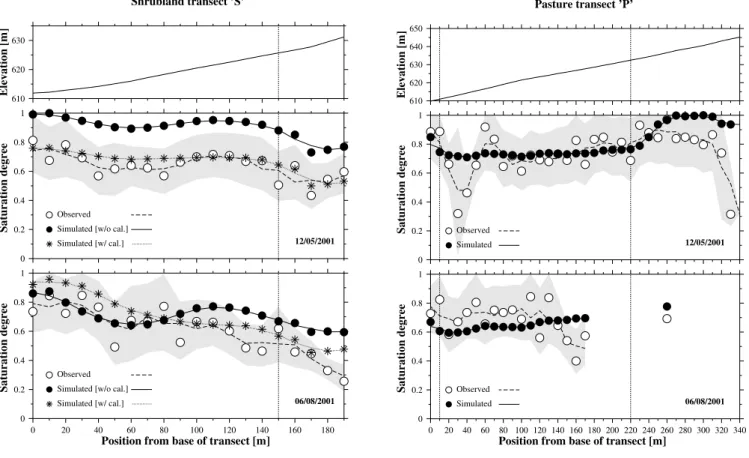
Fig. 6. Comparison between observed (open symbol, dashed line) and simulated (solid symbol and lines) saturation degrees along four
transects,(a)shrubland transect “S”,(b)pasture transect “P”. Simulated results after calibration presented on transect (a) (star symbol, dotted line).
bottom half of the transect, but overpredicted them on the top half, while showing the same generic trend (R2=0.56, NASR=0.21). On 5 December 2001, simulations system-atically overestimated observations by about 33%, but still had a similar trend (R2=0.83, NASR=0.29). These results indicate that the drainage characteristics of the upper por-tion of the transect were underestimated. Indeed, when the average porosity value measured on the site is used instead of the SSURGO estimates, and when the hydraulic con-ductivities at saturation are set to the higher limits reported in the SSURGO database, simulated results have a much better fit to observations, as illustrated Fig. 6a (R2=0.86, NASR=0.09 for 8 June and R2=0.75, NASR=0.06 for 5 De-cember). For the pasture transect “P”, simulated satura-tion degrees are in close agreement with observed moisture contents on both dates (R2=0.43, NASR=0.17 for 8 June and R2=0.04, NASR=0.21 for 5 December). Observed data points at 30 and 330 m on 5 December had suspiciously low measured water content, and are likely outliers. These out-liers explain the low values of theR2. Corresponding error margins were adapted in consequence. Results were also sat-isfactory for transect “F” (forest) on both dates in Fig. 6c,
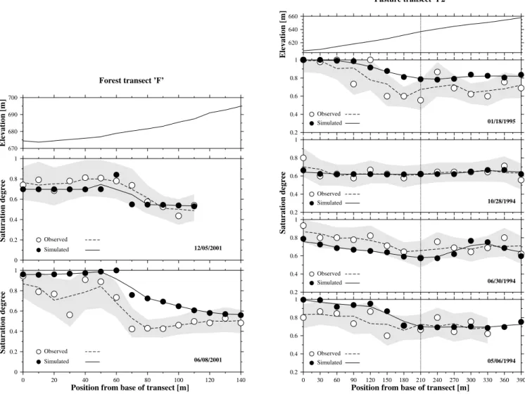
correctly reproducing the observed greater saturation at the flatter base of the slope than on the steeper upper section (R2=0.78, NASR=0.24 for 8 June and R2=0.93, NASR=0.09 for 5 December). On 8 June 2001, however, the model did not reproduce as sharp a decrease in saturation degree with slope change as was observed at 70 m from the bottom of the slope.
Finally, observed saturation degrees (Fig. 6d) were also well reproduced for the fourth transect “P2”, with however a slight systematic overestimation of saturation degrees on 18 January 1995, and overestimation on the bottom part of the transect on 6 June 1994 (R2=0.51 and NASR=0.13 on the four dates).
0 20 40 60 80 100 120 140 0
0.2 0.4 0.6 0.8 1
0 20 40 60 80 100 120 140
0 0.2 0.4 0.6 0.8 1
Position from base of transect [m]
Saturation degree Observed
Simulated 06/08/2001
0 0.2 0.4 0.6 0.8 1
0 0.2 0.4 0.6 0.8 1
Saturation degree Observed
Simulated 12/05/2001
670 680 690 700
Elevation [m]
Forest transect ’F’
0 30 60 90 120 150 180 210 240 270 300 330 360 390 0.2
0.4 0.6 0.8 1
0 30 60 90 120 150 180 210 240 270 300 330 360 390
0.2 0.4 0.6 0.8 1
Position from base of transect [m] Observed
Simulated 05/06/1994
0.2 0.4 0.6 0.8 1
0.2 0.4 0.6 0.8 1
Saturation degree
Observed
Simulated 06/30/1994
0.2 0.4 0.6 0.8 1
0.2 0.4 0.6 0.8 1
Observed
Simulated 10/28/1994
0.2 0.4 0.6 0.8 1
0.2 0.4 0.6 0.8 1
Observed
Simulated 01/18/1995
620 640 660
Elevation [m]
Pasture transect ’P2’
Fig. 6. Continued. (c)forest transect “F”,(d)transect “J”. Symbols: Saturation degrees. Lines: 3-points moving average. Grey stripe:
experimental error. Vertical dash line: soil transition.
entire depth of the soil column. However, it should be noted that the stone content of these soils is high, making it difficult to take samples at deeper depth. Moreover, the spring sam-ples were taken during a relatively dry period, and the winter samples during a relatively wet period. Therefore, a large gradient in moisture content with depth was not expected. Nevertheless, the moisture content for the top soil could sys-tematically underpredict the average moisture content over the whole soil column.
At last, errors originate also from the soil properties input dataset used in the simulation. The SSURGO database de-scribes characteristic soils, and by its statistical nature cannot account for local variability. Therefore, the parameters de-rived from SSURGO are only approximate. A better match of simulations and observations could be achieved by cal-ibrating the soil hydrodynamic characteristics on a soil by soil, or even field by field, basis, as illustrated by the better
fit obtained on transect “S” after calibration. However, such a punctual adjustment of parameters would defy the origi-nal purpose of SMDR, i.e. a fully distributed model that re-quires little calibration, and would lead naturally to the over-parametrization pitfall pointed out by Beven (1996), without gaining much accuracy in the overall location of wet areas. 5.2 Mapping of saturated areas
N
Drains Ditches Streams Old streambed VSAs Fields
0 500
Fig. 7. Position of natural (streams: blue, old streambed:
pur-ple) and artificial (drains: brown, ditches: green) drainage features, and estimated positions of empirical frequently saturated hydro-logic source areas (“wet spots” or VSAs: yellow), as digitized from a 1-m resolution DOQQ.
Fig. 7 (dark grey in Fig. 8). Although the determination of the location and extent of these wet spots is subjective, the structures installed to drain these wet areas are not: they in-clude drainage tile lines (brown orange in Fig. 7 and green in Fig. 8) and open drainage ditches (green in both Figs. 7 and 8). The stream network starting at the saturated areas is also shown in Fig. 7 in blue. The original position of the stream, before its diversion near the barns in the early nineties, is re-ported in purple. In addition, field boundaries (in pink) are also drawn to facilitate comparison and localization of fea-tures.
Simulated daily runoff volumes for the entire period were summed and averaged over the summer (May–October) and winter (November–April) periods, to create the maps in Fig. 8. Note that SMDR calculates runoff as the depth of water in excess of saturation and tile outflow is therefore in-cluded in the simulated runoff. Figure 8a shows that in the summer, most runoff is generated on impervious areas by infiltration excess. Only a small fraction of the pervious ar-eas of the watershed produces runoff in summertime. How-ever, the stream network can still be distinguished. As sur-face runoff is not explicitly routed in SMDR, stream cells are not connected. Since the stream flowing from the pond had water all summer, the agreement is satisfactory. During win-ter the comparison between expected (Fig. 7) and simulated (Fig. 8b) is in general good since all the drainage structures and most of the identified wet spots are within the area gen-erating at least 3 cm/month in average (blue color). This blue area roughly overlays the fragipan-restricted lower terrains. The steeper northeastern slopes produce more runoff than the gentler western slopes. Variable source areas are concen-trated in converging areas, slope breaks, and transition be-tween bedrock- and fragipan-restricted soils. In addition, the streams and the surrounding wet areas generate the higher runoff amounts (shown in black), as expected. A closer
in-N
0 500
0.00 0.05 0.10 0.15 0.20 0.25 0.30 0.35 0.40 0.45
Summer units : [mm]
N
0 500
0.00 0.05 0.10 0.15 0.20 0.25 0.30 0.35 0.40 0.45
Winter units : [mm]
Fig. 8.Seasonal runoff generation on the study watershed,
bound-aries of estimated source areas (grey) and position of drains and ditches (green). (a) Summer (May-October); (b) Win-ter (November-April). Runoff volumes expressed in (mm) (1 mm∼=1637.7 m3).
spection shows that certain features are not predicted well, such as the wet spots on the south east watershed boundary. These wet spots are likely associated with subsurface fea-tures not simulated in the model. Also, part of the stream in the northwest portion of the watershed fades into the back-ground.
6 Conclusions
Results of the hydrological model were good considering the minimal calibration. Hydrographs were generally properly simulated, both in terms of timing and intensity of peaks, although summer baseflows were often underestimated, and some winter peakflows were improperly reproduced. Agree-ment between observed and simulated saturation degrees along four transects at different dates were usually correct. Visual comparison of seasonal cumulative runoff maps and digitized hydrological features was also very encouraging. Improvements should focus on a better representation of snowmelt and soil freezing during winter periods, baseflow generation mechanisms during summer periods, and simple estimation rules for some of the hydrodynamic properties (macroporous drainage limit and horizontal hydraulic con-ductivity). However, given the limited information about spatially distributed nature of soils, the question remains how the suggested improvements can best be implemented to ob-tain more accurate simulated distributed moisture contents.
Acknowledgements. The United States Department of Agriculture, through the National Research Initiative funding, and Department of Interior provided primary funding for this study. The grant of the Department of Interior was administered by the New York State Water Resources Institute. Additional funding was provided by the United States Department of Environmental Protection under the Safe Drinking Water Act, administered by the Watershed Agricul-tural Council (WAC). The data for validation was obtained from P. Bishop of the New York State Department of Environmental Conservation (NYSDEC). M. R. Rafferty, J. L. Lojpersberger of NYSDEC and S. Pacenka of WRI are acknowledged for the collecting and/or modification of this data. In addition, we would like to thank the members of the Town Brook Research Group, Watershed Agricultural Program Planners and Landowners for their invaluable discussions and insights regarding watershed processes in the Catskill Mountains. Specifically we would like to thank the collaborating farm family for their willingness to participate in the research effort and their patience in dealing with us.
Edited by: N. Romano
References
Abbott, M. B., Bathurst, J. C., Cunge, J. A., O’Connell, P. E., and Rasmussen, J.: An introduction to the European hydrological system – Syst`eme Hydrologique Europ´een, “SHE”, 1. history and philosophy of a physically based, distributed modeling sys-tem, J. Hydrol., 87, 45–59, 1986a.
Abbott, M. B., Bathurst, J. C., Cunge, J. A., O’Connell, P. E., and Rasmussen, J.: An introduction to the European hydrological system – Syst`eme Hydrologique Europ´een, “SHE”, 2. structure of a physically based, distributed modeling system, J. Hydrol., 87, 61–77, 1986b.
Allen, R. G., Pereira, L. S., Raes, D., and Smith, M.: Crop evap-otranspiration - Guidelines for computing crop water require-ments – FAO Irrigation and drainage paper 56, FAO – Food
and Agriculture Organization of the United Nations, Rome, IT, http://www.fao.org/docrep/X0490E/X0490E00.htm, 1998. Arnold, J. G., Allen, P. M., and Bernhardt, G.: A comprehensive
surface-groundwater flow model, J. Hydrol., 142, 47–69, 1993. Arnold, J. G., Williams, J. R., Srinivasan, R., King, K. W., and
Griggs, R. H.: SWAT, Soil and Water Assessment Tool, USDA, Agriculture Research Service, Temple, TX 76502, 1994. Beven, K. J.: A discussion of distributed hydrological modelling,
in: Distributed Hydrological Modelling, edited by: Abbott, M. B. and Refsgaard, J. C., Kluwer, Dordrecht, NL, 255–277, 1996. Beven, K. J. (Ed.): Distributed modeling in hydrology: Applica-tions of the TOPMODEL Concept, Adv. Hydrol. Proc. Wiley, Chichester, 1997.
Beven, K. J. and Kirkby, M. J.: A physically based, variable con-tributing area model of basin hydrology, Hydrol. Sci. Bull., 24, 43–69, 1979.
Bicknell, B. R., Imhoff, J. C., Kittle Jr, J. L., Donigian, A. S., and Johanson, R. C.: Hydrological Simulation Program-Fortran: User’s manual for version 11, US Environmental Protection Agency, National Exposure Research Laboratory, Athens, GA, 1997.
Bishop, P. L., Hively, W. D., Stedinger, J. R., Bloomfield, J. A., Rafferty, M. R., and Lojpersberger, J. L.: Multivariate analysis of paired watershed data to evaluate agricultural BMP effects on stream water phosphorus, J. Env. Qual., 34, 1087–1101, 2005. Bishop, P. L., Rafferty, M., and Lojpersberger, J.: Event based
wa-ter quality monitoring to dewa-termine effectiveness of agricultural BMPs, Proceedings of the American Water Resources Associa-tion, International Congress on Watershed Management for Wa-ter Supply Systems, 29 June–2 July, 2003.
Boll, J., Brooks, E. S., Campbell, C. R., Stockle, C. O., Young, S. K., Hammel, J. E., and McDaniel, P. A.: Progress toward de-velopment of a GIS based water quality management tool for small rural watersheds: modification and application of a dis-tributed model, ASAE Annual International Meeting, Orlando, FL., ASAE paper 982230, 1998.
Bresler, E., Russo, D., and Miller, R. D.: Rapid estimate of unsat-urated hydraulic conductivity function, Soil Sci. Soc. Amer. J., 42, 170–177, 1978.
Brooks, R. H., and Corey, A. T.: Hydraulic properties of porous media, Colorado State Univ., Colorado, 1964.
Chiew, F. H. S. and McMahon, T. A.: Application of the daily rainfall-runoff model MODHYDROLOG to 28 Australian catch-ments, J. Hydrol., 153, 383–416, 1994.
DiLuzio, M. D. and Arnold, J. G.: Formulation of a hybrid cali-bration approach for a physically based distributed model with NEXRAD data input, J. Hydrol., 298, 136–154, 2004.
Donigian, A. S., Bicknell, B. R., and Imhoff, J. C.: Hydrological Simulation Program – Fortran (HSPF), Water Resour. Pubs., Col-orado, 1995.
Dunne, T. and Black, R.: Partial area contributing to storm run off in a small New-England watershed, Water Resour. Res., 6, 1296– 1311, 1970.
Dunne, T., Moore, T. R., and Taylor, C. H.: Recognition and pre-diction of runoff-producing zones in humid regions, Hydrol. Sci. Bull., 20, 305–327, 1975.
ESRI: ArcView GIS 3.3, India, 2002.
model, Hydrol. Processes, 13, 805–822, 1999.
Gburek, W. J., Sharpley, A. N., and Pionke, H.: Identification of critical source areas for phosphorus export from agricultural catchments, in: Advances in Hillslope Processes, edited by: An-derson, M. and Brookes, S., John Wiley & Sons, Chichester, UK, 263–282, 1996.
Goudriaan, J. and van Laar, H.H.: Modelling Potential Crop Growth Processes, Textbook with Exercises, Kluwer Academic Publish-ers, 1994.
Haith, D. A., Mandel, R., and Wu, R. S.: Generalized watershed loading functions version 2.0: User’s manual, Tech. rep., Dept. of Agricultural and Biological Engineering, Cornell University, New York, 1992.
Haith, D. A. and Shoemaker, L. L.: Generalized watershed loading functions for stream flow nutrients, Water Resour. Bull., 23, 471– 478, 1987.
Hargreaves, G. H. and Samani, Z. A.: Reference crop evapotranspi-ration from temperature, Appl. Eng. Agric., 1, 96–99, 1985. Hewlett, J. D. and Hibbert, A. R.: Factors affecting the response
of small watersheds to precipitation in humid regions, in: Forest hydrology, edited by: Sopper W. E. and Lull, H. W., Pergamon Press, Oxford, UK, 275–290, 1967.
Hewlett, J.D. and Nutter, W.L.: The varying source area of stream-flow from upland basins, Proc. of the Symp. on Interdisciplinar-ity Aspects of Watershed Mgmt. 08/06/1970, ASCE, Montana, 1970.
Hively, W. D.: Phosphorus loading from a monitored dairy farm landscape, Ph.D. dissertation, Cornell University, Ithaca, NY, 2004.
Horton, R. E.: The role of infiltration in the hydrological cycle, Transactions of the American Geophysical Union, 14, 446–460, 1933.
Horton, R. E.: An approach toward a physical interpretation of in-filtration capacity, Soil Sci. Soc. Amer. Proc., 4, 399–418, 1933. Jensen, M. E., Burman, R. D., and Allen, R. G. (Eds.): Evapotran-spiration and Irrigation Water Requirements, Vol. 70 of ASCE Manuals and Reports on Engineering Practice, American Soci-ety of Civil Engineers, New York, 1990.
Johnson, M. S., Coon, W. F., Mehta, V. K., Steenhuis, T. S., Brooks, E. S., and Boll, J.: Application of two hydrologic models with different runoff mechanisms to a hillslope dominated watershed in the Northeastern US: a comparison of HSPF and SMR, J. Hy-drol., 284, 57–76, 2003.
Kuo, W.-L., Steenhuis, T. S., McCulloch, C. E., Mohler, C. L., We-instein, D. A., DeGloria, S. D., and Swaney, D. P.: Effect of grid size on runoff and soil moisture for a variable-source-area hydrology model, Water Resour. Res., 35, 3419–3428, 1999. Mehta, V. K., Johnson, M. S., G´erard-Marchant, P. G. F.,
Wal-ter, M. T., and Steenhuis, T. S.: Testing a variable source GIS-based hydrology model for watersheds in the northeastern US, the Soil Moisture Routing model, EOS Trans. AGU, 82, Fall Meet. Suppl., Abstract H22I-05, 2001.
Mehta, V. K, Walter, M. T., Brooks, E. S., Steenhuis, T. S., Walter, M. F., Johnson, M. S., Boll, J., and Thongs, D.: Application of smr to modeling watersheds in the Catskills mountains, Env. Model. Assess., 9, 77–89, 2004.
Nash, J. E. and Sutcliffe, J. V.; River flow forecasting through con-ceptual models, part I – a discussion of principles, J. Hydrol., 10, 238–250, 1970.
NCDC: Climatalogical data annual summary – New York, National Climate Data Center (NCDC), North Carolina, 2000.
Neitsch, S. L., Arnold, J. G., Kiniry, J. R., William, J. R., and King, K. W.: SWAT- Soil and Water Assessment Tool, 2000 – Theoret-ical documentation, Texas, 2002.
Neteler, M. and Mitasova, H.: Open Source GIS: A GRASS GIS Approach, Kluwer Academic Publishers, Massachusetts, 2002. NLCD: New York Land Cover Data Set, http://landcover.usgs.gov/
nlcd/show data.asp?code=NY&state=New York, US Geological Survey (USGS), South Dakota, 1997.
NYSDoS: Digitally Enhanced Ortho Imagery Online Link http: //www.nysgis.state.ny.us/gateway/mg/napphtmls/f7.htm, Meta-data: http://www.nysgis.state.ny.us/gis3/data/dos.doqq orthos. html, NYS Department of State Division of Coastal Resources, GIS Unit, New York State, 2000.
Priestley, C. H. B. and Taylor, R. J.: On the assessment of surface heat fluxes and evaporation using large-scale parameters, Mon. Wea. Rev., 100, 81–92, 1972.
Rawls, W. and Brakensiek, D.: Prediction of soil water properties for hydrologic modeling, Watershed Management in the Eight-ies, ASCE, 293–299, 1985.
Refsgaard, J. C. and Knudsen, J.: Operational validation and in-tercomparison of different types of hydrological models, Water Resour. Res., 32, 2189–2202, 1996.
Refsgaard, J. C. and Storm, B.: Computer Models of Watershed Hydrology, edited by: She, M. and Singh, V., Water Resource Publications, Colorado, 1995.
Saulnier, G.-M., Beven, K. J., and Obled, Ch.: Including spatially variable soil depths in TOPMODEL, J. Hydrol., 202, 158–172, 1998.
Schneiderman, E. M., Pierson, D. C., Lounsbury, D. G., and Zion, M. S.: Modeling the hydrochemistry of the Cannonsville water-shed with Generalized Waterwater-shed Loading Functions (GWLF), J. Amer. Water Resour. Assoc., 38, 1323–1347, 2002.
Soil and Water Laboratory: SMDR, the Soil Moisture Distribu-tion and Routing model version 2.0 – DocumentaDistribu-tion, Dept. of Biological and Environmental Engineering, Cornell University, Ithaca, NY, 2003.
Soren, J.: The groundwater resources of Delaware County, New York, Tech. Rep. Water Res. Comm. Bull. GW-50., USGS, New York, 1963.
Srinivasan, M. S., Hamlett, J. M., Day, R. L., Sams, J. I., and Pe-tersen, G. W.: Hydrologic modeling in two subwatersheds of Lake Wallenpaupack, Pennsylvania, J. Amer. Water Resour. As-soc., 34, 963–978, 1998.
Srinivasan, M. S., G´erard-Marchant, P., Veith, T. L., Gburek, W. J., and Steenhuis, T. S.: Watershed-scale modeling of critical-source-areas of runoff generation and phosphorus transport, J. Amer. Water Resour. Assoc., 41, 361–375, 2005.
Steenhuis, T. S. and van der Molen, W. M.: The Thornthwaite-Mather method procedure as a simple engineering method to pre-dict recharge, J. Hydrol., 84, 221–229, 1986.
Tarboton, D. G.: A new method for the determination of flow direc-tions and upslope areas in grid digitale elevation models, Water Resour. Res., 33, 309–319, 1997.
1991.
US Army Corps of Engineers: Engineering and design: Runoff from snowmelt, Tech. Rep. EM 1110-2-1406, US Army Corps of Engineers, Govt. Printing Office, District of Columbia, 1960. US Department of Agriculture, N.R.C.S.: Soil Survey Geographic (SSURGO) database for Delaware County, New York, http:// www.ncgc.nrcs.usda.gov/products/datasets/ssurgo/, 2000. US Geographical Survey (USGS): New York State Digital Elevation
Models (DEM), Davenport quadrangle, Online through Cornell University Geographic Information Resources (CUGIR), Cor-nell University, New York, http://new-gis.mannlib.corCor-nell.edu/ CUGIR Data/data1/u40elu.dem.gz, 1998.
Walter, M. T., Brooks, E. S., McCool, D. K., King, L. G., Mol-nau, M., and Boll, J.: Process-based snowmelt modeling: does it require more input data than temperature-index modeling?, J. Hydrol., 300(1–4), 65–75, 2005.
Walter, M. T., Walter, M. F., Brooks, E. S., Steenhuis, T. S., Boll, J., and Weiler, K. R.: Hydrologically sensitive areas: Variable source area hydrology implications for water quality risk assess-ment, J. Soil Water Conserv., 3, 277–284, 2000.
Western, A.: Comments on “Distributed hydrological modeling of total dissolved phosphorus transport in an agricultural landscape, part 1: Distributed runoff generation” by G´erard-Marchant et al., 2005”, Hydrol. Earth Syst. Sci. Discuss., 2, 1537–1579 RC S780, available online: http://www.cosis.net/copernicus/EGU/hessd/2/ S780/hessd-2-S780.pdf, 2005.
Wigmosta, M. S., Nijssen, B., Storck, P., and Lettenmaier, D.: The Distributed Hydrology Soil Vegetation Model, Mathematical Models of Small Watershed Hydrology and Applications, Water Resource Publications, Colorado, 2002.
Wigmosta, M. S. and Perkins, W. A.: Simulating the effects of for-est roads on watershed hydrology, Land Use and Watersheds: Human Influence on Hydrology and Geomorphology in Urban and Forest Areas, Vol. 2 of Water Science and Application, AGU, 2001.
Wigmosta, M. S., Vail, L., and Lettenmaier, D. P.: A distributed hydrology-vegetation model for complex terrain, Water Resour. Res., 30, 1665–1679, 1994.
Ye, W., Bates, B. C., Viney, N. R., Silvapan, M., and Jakeman, A. J.: Performance of conceptual rainfall-runoff models in low yielding ephemeral catchments, Water Resour. Res., 33, 153–166, 1997. Zollweg, J. A., Gburek, W. J., and Steenhuis, T. S.: SMoRMod - a