Programa de P´
os–Gradua¸c˜
ao em F´ısica
Doutorado em F´ısica
Study of strongly correlated colloidal
systems
Igor Rochaid Oliveira Ramos
Orientador: Prof. Dr. Wandemberg Paiva Ferreira
systems
Igor Rochaid Oliveira Ramos
Tese apresentada ao Departamento de F´ısica da Universidade Federal do Cear´a, como parte dos requisitos para a obten¸c˜ao do T´ıtulo de Doutor em F´ısica.
Banca Examinadora:
Prof. Dr. Wandemberg Paiva Ferreira – UFC (Orientador)
Prof. Dr. Gil de Aquino Farias – UFC
Prof. Dr. Raimundo Nogueira da Costa Filho – UFC
Prof. Dr. Felipe de Freitas Munarin – UFC
Prof. Dr. Fabricio Queiroz Potiguar – UFPA
`
• Inicialmente, agrade¸co a Deus por ter me dado todas as condi¸c˜oes para que eu pudesse realizar este trabalho.
• Ao meu orientador, Prof. Dr. Wandemberg Paiva Ferreira, por toda a aten¸c˜ao, respeito e por ter me ajudado nos momentos mais dif´ıceis deste trabalho.
• A minha esposa, por estar ao meu lado durante todos esses anos.`
• Aos meus pais, Rocha e Eliete, pela vida que me deram e por todo o amparo necess´ario para que eu pudesse chegar at´e aqui.
• Aos meus av´os, Rita Ramos e Miguel Ramos (in memoriam), `a minha tia, Maria Socorro Rocha Ramos, ao meu primo Cirilo, e `a Ester por todo o amor, carinho, e os cuidados dedicados a mim at´e hoje.
• Aos meus tios, Raimundo (in memoriam), Rita, Gilson, Socorro e Concei¸c˜ao, por toda a ajuda durante todos os anos que passei em Fortaleza.
• Ao meu amigo Mardˆonio, pelos seus ensinamentos, direcionamentos e pelo incentivo, desde o pr´e-vestibular.
• Aos amigos, Philipe, S´ılvia, Roberto Namor, Robson e ´Italo que muito me ajudaram durante todos esses anos. Serei eternamente grato.
• Ao Josa (da xerox) pela sua amizade, pelo seu trabalho, e por aceitar os fiados quando o dinheiro acaba.
• Ao chefe do Departamento.
• Aos examinadores da banca, pelas suas corre¸c˜oes e sugest˜oes, que muito enriqueceram este trabalho.
• Aos funcion´arios do Departamento de F´ısica, em especial, a Rejane, Ana Cleide e Creuza.
• Aos professores Dr. Francois Peeters e Dr. Milorad Milosevic por toda a ajuda durante os trˆes meses que fiquei em Antu´erpia.
Resumo
Nesta tese, estudamos as propriedades estruturais e dinˆamicas, bem como, a fus˜ao de sistemas coloidais.
Inicialmente, abordamos o problema de determinar as estruturas de m´ınima energia e o es-pectro de fˆonons de um sistema de dipolos magn´eticos carregados, organizados em uma estrutura de bicamadas e orientados perpendicularmente ao plano das camadas. Este sistema pode ser sin-tonizado atrav´es de seis diferentes fases cristalinas, atrav´es da varia¸c˜ao de parˆametros tais como a separa¸c˜ao entre as camadas e/ou a carga e/ou o momento de dipolo das part´ıculas. A presen¸ca de carga el´etrica nas part´ıculas dipolares ´e respons´avel pela nuclea¸c˜ao de cinco fases onde as ca-madas n˜ao est˜ao alinhadas verticalmente e uma fase desordenada, que n˜ao s˜ao encontradas no sistema em bicamadas de dipolos magn´eticos previamente apresentado na literatura. Estas fases extras s˜ao uma consequˆencia da competi¸c˜ao entre a repuls˜ao coulombiana e a intera¸c˜ao atrativa entre os dipolos em diferentes camadas. As estruturas de m´ınima energia s˜ao sumarizadas em um diagrama de fases associado `a separa¸c˜ao entre camadas e a importˆancia relativa entre as in-tera¸c˜oes el´etrica e magn´etica. Determinamos, ainda, a ordem das transi¸c˜oes estruturais entre as v´arias configura¸c˜oes de m´ınima energia. O espectro de fˆonons do sistema foi calculado usando a aproxima¸c˜ao harmˆonica. Um comportamento n˜ao-monotˆonico do espectro de fˆonons ´e encontrado como fun¸c˜ao da intera¸c˜ao efetiva entre as part´ıculas. A estabilidade termodinˆamica das diferentes fases ´e determinada.
Em seguida, estudamos o sistema de bicamadas de dipolos magn´eticos carregados para tem-peraturas diferentes de zero, investigando a fus˜ao do sistema atrav´es do crit´erio de Lindemann modificado, em fun¸c˜ao dos parˆametros: (i) a distˆancia entre as camadasη e (ii) a intensidade rel-ativa da intera¸c˜ao magn´etica com respeito `a intera¸c˜ao el´etrica λ. Para λ suficientemente grande, uma das fases (a fase hexagonal com alinhamento vertical) exibe um comportamento reentrante na temperatura de fus˜ao em fun¸c˜ao deη. Uma vez que a carga e o momento de dipolo magn´etico das part´ıculas coloidais pode ser alterado, por exemplo, pela varia¸c˜ao do pH da solu¸c˜ao na qual est˜ao imersos e por um campo magn´etico externo, respectivamente, este sistema pode ser em princ´ıpio verificado experimentalmente.
This thesis presents the study of the structural and dynamical properties, as well as, melting of colloidal systems.
Initially, we study the structure and phonon spectrum of a system of charged magnetic dipoles, organized in a bilayer structure and oriented perpendicular to the plane of the layers. This system can be tuned through six different crystalline phases by changing parameters such as the interlayer separation and/or the charge and/or dipole moment of the particles. The presence of the electric charge on the dipole particles is responsible for the nucleation of five staggered phases and a disordered phase which are not found in the magnetic dipole bilayer system previously presented in the literature. These extra phases are a consequence of the competition between the repulsive Coulomb and the attractive dipole interlayer interaction. The minimum energy structures are summarized in a phase diagram associated to the separation between the layers and to the relative importance between the magnetic and electric interactions. We determine the order of the structural phase transitions. The phonon spectrum of the system was calculated within the harmonic approximation. A non-monotonic behavior of the phonon spectrum is found as a function of the effective strength of the inter-particle interaction. The thermodynamic stability of the different phases is determined.
Then, we study the bilayer system of charged magnetic dipoles for nonzero temperatures, investigating the melting behavior of the system through the modified Lindemann criterion, as a function of the parameters: (i) the distance between the layers η and (ii) the relative intensity of the magnetic interaction with respect to the electric interaction λ. For large enough λ, one of the phases (the matching hexagonal phase) exhibits a re-entrant melting behavior as a function of η. Since the charges and the magnetic dipole moment of the colloidal particles can be altered, for example, by changing the pH of the solution in which they are immersed or an external magnetic field, respectively, this system can be in principle verified experimentally.
1 Introduction 2
1.1 Colloidal systems . . . 2
1.2 Structure of the thesis . . . 5
2 Bilayer crystals of charged magnetic dipoles: structure and phonon spectrum 6 2.1 Introduction . . . 6
2.2 Model . . . 8
2.3 Ground state crystal structures . . . 14
2.4 Dynamical Properties . . . 19
2.5 Conclusions . . . 32
3 Melting of a classical bilayer crystal of charged magnetic dipoles 34 3.1 Introduction . . . 34
3.2 Classical melting . . . 35
3.2.1 Analytical calculations . . . 36
3.3 Results and discussion . . . 41
3.4 Conclusions . . . 45
4 Dynamical properties and melting of binary two-dimensional colloidal alloys 47 4.1 Introduction . . . 47
4.2 Model . . . 49
4.3 Dynamical properties . . . 53
4.4 Melting . . . 65
4.5 Conclusions . . . 71
5 Conclusions 73 A Energy per particle using Ewald summation 75 A.1 Electric case . . . 75
1.1 One component monolayers of silica particles with diameter (a) 3µm and (b) 1µm at a horizontal octance/water interface. The scale bars are equal to 30µm and the average distance between large particle centers in (a) is 28µm. Figure taken from Ref. [5]. . . 3 1.2 pH-dependence of the superficial density of charge. For pH≤3.5 in acidic medium
and pH≥10.5 in basic one, the nanoparticles are charge saturated and the ferrofluid is thermodynamically stable. Figure taken from Ref. [10]. . . 4
2.1 Top view of the structures of the ordered phases, where the circles (crosses) corre-spond to the lower (upper) layer. In the case of the matched phases, the layers are not displaced and are exactly on top of each other, as is shown for the MH phase. 15 2.2 (a) The total energy per particle (in units of E0 =Q2√n) as function of η for the
different phases presented in Table 2.1. (b) Detailed view of (a). (c) The sine of the angle between the primitive vectors⃗a1 and⃗a2 of the SRhomb phase as a function of
η. The inset in (c) shows how the aspect ratio a2/a1 for the SRect phase depends
onη. . . 16 2.3 The zero temperature phase diagram where λ = µ2n/Q2 and η = d√
n/2. First (second) order structural phase transitions are indicated by solid (dotted) lines. The labels indicating the crystalline phases are given in Table 2.1. The hatched area corresponds to the disordered phase. . . 17 2.4 The log ×log plot of the critical λ(η) curve which separates the staggered phases
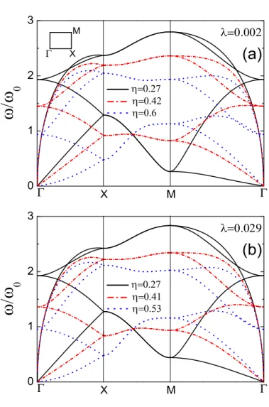
from the MH phase taken from Fig. 2.3. . . 18 2.5 The phonon spectrum for the staggered square phase for different values of η and
for (a)λ= 0.002 and (b)λ= 0.029. The high-symmetry directions of the reciprocal space are presented in the inset. The frequency is in units of ω0 =Qn3/4/m1/2. . 22
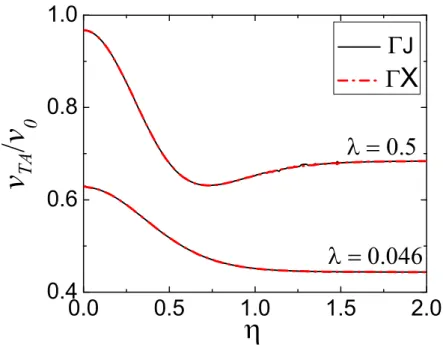
2.6 The phonon spectrum for the MH phase for different values ofη and fixed λ. The high-symmetry directions of the reciprocal space are presented in the inset. . . . 24 2.7 The sound velocity (in units of v0 =ω0/√n) of the TA mode as a function ofη for
2.8 The phonon spectrum for the SH and MH phase for different λ and fixed η = 0.8. The high-symmetry direction of the reciprocal space are presented in the inset. . . 27 2.9 The phase boundaries (circles) and the range of stability (colored triangles) for the
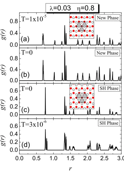
different phases as a function of η for two values of λ. Closed (open) circles refer to first (second) order structural phase transitions. . . 28 2.10 The radial distribution function as calculated from our MC simulations for the new
phase and the SH phase for two different temperatures. For the new phase: (a) T = 1×10⁻⁵ and (b) T = 0. For the SH phase: (c) T = 0 and (d) T = 3×10⁻⁶.
The configuration of the new phase (energyE =−1.340575) is presented as inset in (a), while the configuration of the SH phase (energy E =−1.340534) is presented as inset in (c). The T ̸= 0 results in (a) and (d) were obtained by applying MC simulations starting with the new phase and the SH phase at T = 0, respectively. Solid and open circles represent particles in distinct layers. . . 29 2.11 The radial distribution function as calculated from our MC simulations (T = 0)
taking into account only one layer of the SH phase (dash-dotted black curve) and one layer of the new phase (solid red curve). . . 31
3.1 Melting temperature of the energetically favorable phases as a function ofη, for (a) λ= 0.01 and (b) λ= 0.03 . The vertical dotted lines indicate the phase boundaries. 42 3.2 Melting temperature of the SH and MH phases for η= 0.8 as a function ofλ. The
vertical dotted lines indicate the phase boundaries. . . 43 3.3 Melting temperature of the MH phase as a function of η. . . 44 3.4 Melting temperature of the SS phase for three values of η as a function of λ. . . . 44
4.1 Structures of the colloidal alloys (a)AB2 (b) AB3 (c) AB5 (d)AB6 and (e)S(AB).
The unit cell of each phase is shown by the solid box and the primitive vectors are explicitly shown. . . 49 4.2 Two silica particles of different size floating at an oil-water interface. The charges
at the particle-oil interface generate a resultant dipole moment in each particle. . 51 4.3 A material with four magnetic domains where the vectors indicate the magnetic
dipoles. . . 52 4.4 Example of a spherical multi-domain particle for (a)D > Dc and of a mono-domain
particle for (b)D < Dc, whereDis the diameter of the particle andDc is the critical
diameter. . . 53 4.5 Super-paramagnetic colloidal particles at a water-air interface. An external
4.6 Square of the phonon frequencies of the crystal phaseAB2 for m∗ =sB in units of
ω2
0 =µ2Aρ
5/2
A /mA (a) for sB = 0.015 and (b) sB = 0.037, along the high-symmetry
directions in reciprocal space. The high-symmetry points Γ, J andX are shown in the inset of (b). Only the lowest energy modes are shown in (b) in order to enlarge the region around zero frequency. . . 58 4.7 Square of the phonon frequencies of the phase AB2 for m∗ = 1 (a) for sB = 0.015
and (b)sB = 0.037. Only the lowest energy modes are shown in (b). . . 58
4.8 Square of the phonon frequencies of the phase AB2 considering m∗ = 1 ((a) and
(b)) and m∗ =s
B ((c) e (d)). . . 59
4.9 Square of the phonon frequencies of the phase AB6 for sB = 0.002 in units of
ω2
0 =µ2Aρ
5/2
A /mA for (a) m∗ =sB and (b) m∗ = 1. . . 60
4.10 Dispersion relation of the phase S(AB) for sB = 0.25 along the high-symmetry
directions in reciprocal space (a) for m∗ = s
B and (b) for m∗ = 1. The
high-symmetry points Γ,X and M are shown in the inset of (b). . . 62 4.11 The sound velocity in units of ν0 = ω0/√ρA of the transverse acoustical mode of
the phase AB2 as a function of sB for m∗ = 1 andm∗ =sB. . . 63
4.12 The sound velocity in units of ν0 = ω0/√ρA of the transverse acoustical mode of
the phase AB6 as a function of sB for m∗ = 1 andm∗ =sB . . . 63
4.13 The sound velocity in units of ν0 = ω0/√ρA of the transverse acoustical mode of
the S(AB) as a function of sB for m∗ = 1 andm∗ =sB. . . 64
4.14 (a) The optical frequencies in units ofω0 at the Γ point forAB2 as a function ofsB
form∗ =s
B (dotted line) and m∗ = 1 (short dash dotted line) and (b) positions of
the small particles inside the unit cell of the structure AB2 as a function of sB. . . 65
4.15 The optical frequencies in units of ω0 at the Γ point for AB6 as a function of sB for
m∗ =s
B and m∗ = 1. . . 66
4.16 The optical frequencies in units of ω0 at the Γ point forS(AB) as a function ofsB
for m∗ =s
B and m∗ = 1. . . 66
4.17 Melting temperature of the A sub-lattice of the phase AB2 as a function of the
dipole moment ratio. m∗ = 1 (m∗ = sB) means particles A and B with equal
(different) masses. For m∗ = 1, the melting temperature assumes the maximum
value 1/ΓM = 0.01507 for sB = 0.0231. . . 69
4.18 Melting temperature of the A sub-lattice for the structure AB6 as a function of
the dipole moment ratio. m∗ = 1 (m∗ =s
B) means particles A and B with equal
(different) masses. The melting temperature form∗ = 1 reaches its maximum value
4.19 Melting temperature of the Asub-lattice for the configuration S(AB) as a function of the dipole moment ratio. Here, form∗ = 1, the maximum temperature 1/Γ
M ≈
0.060 takes place for sB = 0.18, while for m∗ = sB, the maximum temperature
2.1 Lattice parameters of the different crystalline structures. a is the average nearest neighbor distance which is determined by the density and the configuration (see last column). For each case,⃗a1 and⃗a2 are the primitive lattice vectors, and⃗cis the
interlattice displacement vector.⃗b1and⃗b2are the primitive vectors of the reciprocal
lattice, n is the density. The aspect ratio of phases II and VII is α = a2/a1. In
phases IV and IX, the angle between the lattice vectors⃗a1 and⃗a2 is θ. . . 14
4.1 Interval of stability of some colloidal alloys. The phasesAB3 and AB5 are unstable and therefore are not listed. . . 61
4.2 Fitting parameters for the sound velocity of the phase AB2. . . 62
4.3 Fitting parameters for the sound velocity of the phase AB6. . . 64
Introduction
1.1
Colloidal systems
The term colloidal system or colloidal suspension is frequently used when one deals with materials that are composed of particles of typical sizes varying between 1 nm and 1 µm, called mesoscopic particles, dispersed into a solvent whose molecules are much smaller in size. The mesoscopic particles form the disperse phase and the solvent, the dispersion medium. In the case of a solid disperse phase composed of magnetic nanoparticles which are distributed into a liquid dispersion medium, this colloidal magnetic system is termed ferrofluid or magnetic fluid.
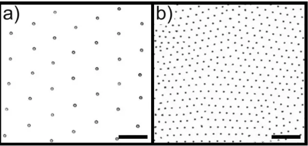
This type of system has attracted the attention of many reseachers in the last decades. The main reasons of the importance of the system of colloids are the following: 1) unlike atomic systems in which the interactions between the particles are determined by their electronic structure and therefore can not be controlled externally [1, 2], the interactions between colloidal particles and, thus, the physical properties of the system, can be modified externally by controlling, for example, the temperature, the salt concentration, the composition (stoichiometry) of the system and/or an external magnetic field, depending on the type of particle in the system; 2) from the experimental point of view, the size of the colloidal particles is of the order of magnitude of the wavelength of visible light (400 nm - 700 nm) and, thus, one can study this system through light scattering experiments [1, 2]. Besides, the particle motion can be observed directly using video microscopy and, therefore, the state of the system can be studied in real time [3, 4]. For example, in Figure 1.1, we have one-component monolayers of silica particles with diameter 3µmand 1µmat a horizontal octane/water interface, which were observed from above using video microscopy [5].
Figure 1.1: One component monolayers of silica particles with diameter (a) 3µm and (b) 1µm at a horizontal octance/water interface. The scale bars are equal to 30µm and the average distance between large particle centers in (a) is 28µm. Figure taken from Ref. [5].
Coulomb potential.
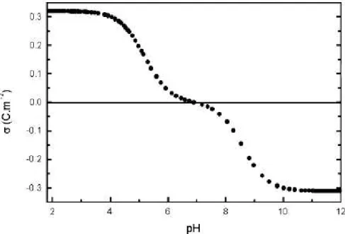
On the other hand, in an electrically stabilized colloidal system, the charge of the colloids can be controlled by the pH of the solution by adding/removing salt to/from the solvent [9, 10]. For instance, in Fig. 1.2, we have the pH-dependence of the superficial density of charge of a ferrofluid based on cobalt ferrite nanoparticles. We can see that, for pH values around 3.5 and 10.5, the nanoparticles are charge saturated and the ferrofluid is thermodynamically stable [10].
In a system composed of super-paramagnetic colloidal particles, the interaction can be altered by changing the applied external magnetic field. Due to the super-paramagnetic character of the particles, thermal fluctuations of the magnetic moment around the preferred direction are negli-gible, i. e., the magnetic dipole of each particle aligns perfectly with the external field. Besides, the strength of the induced dipole moment can be tuned by the magnitude of the external mag-netic field [11]. If the system has super-paramagmag-netic particles of different sizes, the composition (for example, the concentration of small particles) can be used to modify the interaction between the particles. Therefore, colloidal systems are very much used as model systems to study, for instance, melting, because the size of colloidal particles and their interactions can be tailored for experimental studies [2, 12, 13, 14].
Figure 1.2: pH-dependence of the superficial density of charge. For pH ≤ 3.5 in acidic medium and pH ≥10.5 in basic one, the nanoparticles are charge saturated and the ferrofluid is thermo-dynamically stable. Figure taken from Ref. [10].
validity of a melting theory, for instance, the two-dimensional (2D) Kosterlitz-Thouless-Halperin-Nelson-Young (KTHNY) theory. According to this theory, melting is based on the decoupling of pairs of topological defects and it predicts the existence of an intermediate equilibrium phase - the
hexatic phase - between the crystal and the liquid phase [14]. In the hexatic phase, the system
has no translational order while the orientational correlation is still quasi-long-range. Such a two step melting is not known in 3D for isotropic pair interactions [4]. The theoretical melting scenario according to the KTHNY theory was confirmed experimentally using a one-component system of super-paramagnetic colloidal particles at an water-air interface, in the presence of an external magnetic field, and interacting through a repulsive dipole-dipole potential [14]. Although this system of interacting dipole particles is very well understood in the classical regime, it was unknown whether the hexatic phase exists when the quantum fluctuations play a major role. An estimate of the effect of quantum fluctuations on this hexatic phase was presented for both dipolar systems and charged Wigner crystals, predicting that the hexatic phase is stable to very low temperatures [15].
the phonon gaps can be controlled by changing the susceptibility ratio, the composition, and the mass ratio between the two components [16].
Besides melting and phonons, the structural phases in colloidal system is also frequently in-vestigated. For instance, Law et al. [5], reported experimental studies on a 2D binary colloidal system composed of silica particles of different sizes floating at an oil-water interface, and interact-ing through a repulsive dipole-dipole potential. In this case, the interaction between the particles can be modified by changing the size of the colloidal particles.
The examples cited above help us to understand the main reasons of the importance of colloidal systems: the interaction between the particles can be externally controlled and the possibility of experimental access. This understanding is crucial for the appreciation of the next chapters since we will deal with the structural and dynamical properties of some colloidal systems.
1.2
Structure of the thesis
Bilayer crystals of charged magnetic
dipoles: structure and phonon spectrum
2.1
Introduction
Strongly repulsive interacting particles crystallize for a certain range of density and temper-ature. This has been found in systems of rather different nature and therefore the study of the structural and dynamical properties of such a crystalline phase is of fundamental interest. The crystallization phenomenon of strongly interacting particles was originally predicted for an electron gas (Wigner crystal - WC) by E. P. Wigner in 1934 [17]. Up to now, the original three-dimensional (3D) WC of electrons is not yet observed experimentally, mainly due to defects and imperfections in real lattice structures. But experimental evidence of the WC was found in 1979 in a 2D system of electrons on the surface of liquid helium [18]. Nowadays, the term Wigner crystal is used in a broad sense for the crystalline state of clusters of strongly interacting particles. Such Wigner crystallization has also been observed in atomic and molecular clusters [19, 20, 21] and in several non-electronic classical systems as colloids [12, 5, 22, 23, 24, 16], complex dusty plasma [30], and metallic spheric balls [31].
For the particular case of classical systems (e. g., charged or magnetic colloidal particles [32]), crystallization is observed if the interaction potential energy overcomes the kinetic energy of the particles and correlation effects dominate the long-range structure of the system [33]. More specifically, the thermodynamic state of the system is characterized by the coupling parameter Γ, defined as the average of the ratio between the interaction potential energy and the kinetic energy. For a 2D classical system of charged particles with Coulomb interaction, Γ =q2√πn/k
BT, where
q is the charge of each particle,n the density,kB the Boltzmann constant and T the temperature.
particles become strongly correlated and the system typically changes to a crystalline phase for Γ∼130.
In a 2D system of purely repulsive interacting particles the ground state configuration is found to be the hexagonal lattice [34, 35]. However, a more interesting scenario is observed if a 2D system of particles with pure repulsive interaction are arranged in a bilayer structure. In this case, the set of possible ground state configurations is richer, and many other 2D structures, not observed in the single-layer case, now appear as the minimum energy configuration. Goldoni and Peeters [36] showed that the hexagonal lattice is the ground state only when the separation between layers is zero or larger than a critical value. In the latter case, the hexagonal lattice in each layer are displaced with respect to each other (staggered hexagonal phase). For intermediate distances between the layers, staggered square, rectangular, and rhombic phases become the ground state.
In a 2D system of magnetic dipoles oriented perpendicularly to the layers, Xin Lu et al.
[37] showed that, independently of the distance between the layers, the hexagonal phase is the minimum energy structure in each layer, and the dipoles in the different layers are aligned along the direction perpendicular to the layers (matching hexagonal phase). In addition, a reentrant melting temperature, which was related to the anisotropic nature of the dipole interaction, was predicted in this case. Magnetic 2D system of colloidal particles appear yet in many interesting recent studies [5, 24, 38, 39, 40].
Motivated by modern technical methods of synthetizing particles and the assembly of colloidal particles in controlled structures [41], we study a 2D classical bilayer system of charged magnetic dipoles directed perpendicular to the layers (which can be realized by the application of a magnetic field). Such particles have recently been produced using magnetic colloidal particles [12] with electrical stabilization [9]. Note that in an electrically stabilized colloidal system the charge of the colloids can in principle be controlled by the PH of the solution by adding/removing salt to/from the solvent [10]. Furthermore, the magnetic moment of the paramagnetic particles is tunable by the strength of the external magnetic field. In a single layer, both the Coulomb and the magnetic interaction lead to a repulsion between the particles favoring the formation of a 2D Wigner lattice. Between the layers the particles exert a repulsive Coulomb interaction while the magnetic interaction is attractive. Depending on the relative strength between the magnetic and Coulomb interaction, the particles in both layers can be either staggered or on top of each other. Here, we study the ground state configurations and the frequencies of the phonon modes as a function of the separation between the layers and a parameter which is related to the ratio between the dipole moment (µ) and the charge (Q) of the particles (λ = µ2n/Q2, with n the
density of particles).
separation between the layers and λ. In Sec. 2.4 we present the methodology used to calculate the phonon spectrum and discuss the numerical results. Our conclusions are given in Sec. 2.5.
2.2
Model
We study a two-dimensional classical crystal of charged dipole particles with total density n arranged in a bi-layer structure. The particles are evenly distributed over the layers (xy plane), which are separated by a distance d along the z-axis. Each particle has charge Q and magnetic dipole moment ⃗µ=µˆez oriented perpendicular to the layers. Thus, the inter-particle interaction
consists of a repulsive Coulomb term Q2/|⃗r
1−⃗r2| and a dipole interaction termµ2/|⃗r1−⃗r2|3. For
convenience we included the dielectric constant ϵ of the medium into Q2 and therefore, Q/√ϵ is
the real charge of the particles (Fig. 2.1).
In order to confine the colloidal particles in each layer into a plane we can make use of, e. g., glass plates. Because of the difference between the dielectric constants of the glass plates and the water environment in which the colloids are, it will lead to image charges as discussed in Ref. [42]. But because the dielectric constant of water (ϵ = 80) is much larger than of the confining glass plates, the induced image charges have the same charge as the colloidal particles. This will have two effects: 1) the colloidal particles will be repelled by the glass plates and will therefore form a 2D layer in the middle between the two glass plates, and 2) the inter-colloid repulsive interaction will increase which can, to some extent, be modeled by replacing the charge Q by an effective charge Q∗ > Q. Therefore, including this dielectric mismatch effect will not qualitatively modify
our results.
Typically, we consider colloidal particles containing magnetic ions exhibiting paramagnetic behavior and thus a magnetic field is applied in thez-direction aligning all magnetic moments in the z-direction. The considered crystal structures are 2D lattices in which the unit cell consists of two particles, one in each layer, where we will label the lattices in different layers by A and B (Fig. 2.1). The equilibrium positions of the particles in each layer are given by R⃗A =l1⃗a1+l2⃗a2,
and R⃗B =l1⃗a1+l2⃗a2+⃗c, where l1 and l2 are integers,⃗a1 and⃗a2 are the primitive vectors,⃗cis a
two-dimensional vector which describes the shift of lattice B with respect to A in the xy plane. For ⃗c = 0 the lattices are not displaced, and are exactly on top of each other (matched case). The case⃗c̸= 0 implies staggered lattices. Because of equal density of particles in both layers, the lattice structure in both layers is the same.
The total interaction energy is given by
with the Coulomb interaction energy
Eelt =1 2
∑
RA̸=R′A
Q2 |R⃗A−R⃗′A|
+ 1 2
∑
RB̸=R′B
Q2 |R⃗B−R⃗′B|
+ ∑
RA,RB
Q2
√
|R⃗A−R⃗B|2+d2
,
(2.2)
where d is the separation between the layers. The dipole-dipole interaction energy is
Emagt =1 2
∑
RA̸=R′A
µ2 |R⃗A−R⃗′A|3
+1 2
∑
RB̸=R′B
µ2 |R⃗B−R⃗′B|3
+ ∑
RA,RB
µ2(|R⃗A−R⃗B|2−2d2)
[|R⃗A−R⃗B|2+d2]
5 2
.
(2.3)
Since the layers are equivalent, it is convenient to write the total energy per particle E as
E = E
t
N =Eel+Emag, (2.4)
where the total Coulomb (Eel) and magnetic (Emag) energy per particle can be split as
Eel =
1
2(E0E+EIE), (2.5a)
Emag =
1
2(E0M +EIM), (2.5b)
where
E0E =
∑
⃗ R̸=⃗0
Q2
|R⃗|, (2.6a)
E0M =
∑
⃗ R̸=⃗0
µ2
|R⃗|3, (2.6b)
are the Coulomb and magnetic interaction energy per particle in each layer, respectively, and ⃗
R =l1⃗a1+l2⃗a2. On the other hand,
EIE =
∑
⃗ R
Q2
(|R⃗ +⃗c|2+d2)1/2, (2.7a)
EIM =
∑
⃗ R
µ2(|R⃗ +⃗c|2−2d2)
(|R⃗ +⃗c|2+d2)5/2 , (2.7b)
respectively. Following the procedure developed in Refs. [34, 35, 36, 37], we define the auxiliary functions (see Appendix A):
T0(⃗r, ⃗q) = e−i⃗q·⃗r
∑
⃗ R
ei⃗q·(⃗r−R⃗) |⃗r−R⃗| −
1
r, (2.8a)
TI(⃗r, ⃗q) = e−i⃗q·⃗r
∑
⃗ R
ei⃗q·(⃗r−R⃗+⃗c)
[|⃗r−R⃗ +⃗c|2+d2]1/2, (2.8b)
ψ0(⃗r, ⃗q) = ei⃗q·⃗r
∑
⃗ R̸=⃗0
e−i⃗q·(⃗r+R⃗)
|⃗r+R⃗|3 , (2.8c)
ψI(⃗r, ⃗q) = ei⃗q·⃗r
∑
⃗ R
(
e−i⃗q·(⃗r+R⃗+⃗c) |⃗r+R⃗ +⃗c|3 +
−3d2e−i⃗q·(⃗r+R⃗+⃗c) |⃗r+R⃗ +⃗c|5
)
.
(2.8d)
The function ψI(⃗r, ⃗q) can also be written as
ψI(⃗r, ⃗q) = ψI1(⃗r, ⃗q)−3d2ψI2(⃗r, ⃗q) (2.9)
with
ψI1(⃗r, ⃗q) =
∑
⃗ R
e−i⃗q·(R⃗+⃗c)
|⃗r+R⃗ +⃗c|3, (2.10a)
ψI2(⃗r, ⃗q) =
∑
⃗ R
e−i⃗q·(R⃗+⃗c)
|⃗r+R⃗ +⃗c|5, (2.10b)
where |⃗r+R⃗ +⃗c| ≡ (|⃗r+R⃗ +⃗c|2 +d2)1/2. Using Eqs. (2.8 - 2.10) we can write Eqs. (2.6) and
(2.7) as
E0E =Q2lim
⃗r→0T0(⃗r,⃗0), (2.11a)
EIE =Q2lim
⃗r→0TI(⃗r,⃗0), (2.11b)
E0M =µ2lim ⃗
r→0ψ0(⃗r,⃗0), (2.11c)
EIM =µ2lim ⃗
r→0ψI(⃗r,⃗0). (2.11d)
Eqs. (2.8a) and ( 2.8b) are re-written as [34, 35, 36]
T0(⃗r, ⃗q) =
√
n/2∑
⃗ G
e−i(⃗q+G⃗)·⃗rΦ
(
|⃗q+G⃗|2
2πn
)
+ √n/2∑
⃗ R̸=⃗0
e−i⃗q·R⃗Φ(πn|⃗r−R⃗|2/2) + √n/2Φ(πn|⃗r|2/2)− 1
r, (2.12a)
TI(⃗r, ⃗q) =
√
n/2∑
⃗ G
e−i(⃗q+G⃗)·⃗re−i ⃗G.⃗cΨ
(
|⃗q+G⃗|2
2πn , πη
2
)
+ √n/2∑
⃗ R
e−i⃗q·(R⃗−⃗c)Φ(π[n|⃗r−R⃗ +⃗c|2/2 +η2]),
(2.12b)
where G⃗ are arbitrary reciprocal lattice vectors given by G⃗ =l1⃗b1+l2⃗b2 (l1, l2 are integers) and
⃗b1,⃗b2 are the primitive translation vectors of the reciprocal lattice. The functions
Φ(x) =
√
π xerfc(
√
x) , (2.13)
and
Ψ(x, y) = 1 2
√
π x[e
√
4xyerfc(√x
+√y) +e−√4xyerfc(√x−√y)]
(2.14)
rapidly converge to zero for large values of their arguments. The term erfc(x) is the complementary error function, and η = d√n/2 is a dimensionless parameter proportional to the separation between the two layers. By considering Eqs. (2.13) and (2.14), Eqs. (2.11a) and (2.11b) can be written as
E0E =Q2
√
n/2A , (2.15)
where
A= 2∑
⃗ R̸=⃗0
Φ(πn|R⃗|2/2)−4, (2.16)
and
EIE =Q2
√
where,
B(η) = ∑
⃗ R
Φ(π[n|R⃗ +⃗c|2/2 +η2])
+∑
⃗ G̸=⃗0
e−i ⃗G·⃗cΨ
(
|⃗q+G⃗|2
2πn , πη
2
)
+ 2{πη·erfc(√πη)−e−πη2}.
(2.18)
A similar approach is considered for the magnetic interaction. In this case, following Ref. [37], the following expressions are obtained
ψ0(⃗r, ⃗q) =
πn 2
∑
⃗ G
ei(⃗q+G⃗)·⃗r
[
4ε
√
πe
−|⃗q+G⃗|2/4ε2
− 2|⃗q+G⃗|erfc
(
|⃗q+G⃗| 2ε
)]
+
[
2εe−ε2r2
√
πr2 −
erf(εr) r3
]
+∑
⃗ R̸=⃗0
e−i⃗q·R⃗
[
erfc(ε|R⃗ +⃗r|)
|R⃗ +⃗r|3
+ ( 2ε √ π )
e−ε2
|R⃗+⃗r|2
|R⃗ +⃗r|2
]
,
(2.19a)
ψI(⃗r, ⃗q) =
πn 2
∑
⃗ G
ei(⃗q+G⃗)·⃗rei ⃗G·⃗c
[
4ε
√
πe
−|⃗q+4εG⃗2|2−ε 2
d2
− e−|⃗q+G⃗|d|⃗q+G⃗|erfc
(
|⃗q+G⃗| 2ε −εd
)
− e|⃗q+G⃗|d|⃗q+G⃗|erfc
(
|⃗q+G⃗| 2ε +εd
)]
+∑
⃗ R
e−i⃗q·(R⃗+⃗c)
[
erfc(ε|R⃗ +⃗c+⃗r|)
|R⃗ +⃗c+⃗r|3
+
(
2ε
√π
)
e−ε2
|R⃗+⃗c+⃗r|2
|R⃗ +⃗c+⃗r|2 −3d 2
(
erfc(ε|R⃗ +⃗c+⃗r|)
|R⃗ +⃗c+⃗r|5
+
(
2ε 3√π
)
(3 + 2ε2|R⃗ +⃗c+⃗r|2)e−ε2
|R⃗+⃗c+⃗r|2
|R⃗ +⃗c+⃗r|4
)]
,
where|R⃗+⃗c+⃗r| ≡(|R⃗+⃗c+⃗r|2+d2)1/2 , and the parameter ε >0 is related to the inverse of the average distance between particles in the same layer, i.e., ε = 1/r0 =
√
πn/2. In this case, Eqs. (2.11c) and (2.11d) can be written, respectively, as
E0M =µ2(n/2)3/2C, (2.20)
where
C =∑
⃗ G
[
4πe−|G⃗|2/2πn− √2|G⃗|π
n/2erfc
(
|G⃗| 2√πn/2
)]
+∑
⃗ R̸=⃗0
[
erfc(√πn/2|R⃗|) (n/2)3/2|R⃗|3 +
(
4 n
)
e−πn|R⃗|2/2
|R⃗|2
]
−4π3 ,
(2.21)
and
EIM =µ2(n/2)3/2D(η), (2.22)
where
D(η) =∑
⃗ G
ei ⃗G·⃗c
[
4πe−|
⃗ G|2 2πn−πη
2
− √π|G⃗|
n/2e
−|G⃗|η/√n/2erfc
(
|G⃗| 2√πn/2 −
√
πη
)
− √π|G⃗|
n/2e
|G⃗|η/√n/2erfc
(
|G⃗| 2√ πn/2+ √ πη )] +∑ ⃗ R [
erfc(√πn/2|R⃗ +⃗c|) (n/2)3/2|R⃗ +⃗c|3
(
1− 6η
2
n|R⃗ +⃗c|2
)
+ 4e−
πn|R⃗+⃗c|2/2
n|R⃗ +⃗c|2
(
1− 6η
2
n|R⃗ +⃗c|2 −2πη 2
)]
.
(2.23)
Finally, the total energy per particle defined in Eq. (2.4) can be written as
E Q2√n =
1
2√2(A+B(η)) + µ2n
Q2
1
25/2(C+D(η)). (2.24)
Now we define the dimensionless parameter
λ = µ
2n
Q2 (2.25)
Phases ⃗a1
a
⃗a2
a ⃗c
⃗b1a
2π
⃗b2a
2π
na2
2
I. one-component hexagonal (OCH) (1,0) (0,√3) ⃗a1+⃗a2
2 (1,0) (0,1/ √
3) √1 3
II. staggered rectangular (SRect) (1,0) (0, α) ⃗a1+⃗a2
2 (1,0) (0,1/α)
1
α
III. staggered square (SS) (1,0) (0,1) ⃗a1+⃗a2
2 (1,0) (0,1) 1
IV. staggered rhombic (SRhomb) (1,0) (cosθ,sinθ) ⃗a1+⃗a2
2 (1,− cosθ
sinθ ) (0,
1 sinθ)
1 sinθ
V. staggered hexagonal (SH) (1,0) (12,√23) ⃗a1+⃗a2
3 (1,− 1
√
3) (0, 2 √ 3) 2 √ 3
VI. matching hexagonal (MH) (1,0) (12,√23) 0 (1,√−1
3) (0, 2 √ 3) 2 √ 3
VII. matching rectangular (MRect) (1,0) (0, α) 0 (1,0) (0,a1
a2)
1
α
VIII. matching square (MS) (1,0) (0,1) 0 (1,0) (0,1) 1
IX. matching rhombic (MRhomb) (1,0) (cosθ,sinθ) 0 (1,−sincosθθ) (0,sin1θ) sin1θ Table 2.1: Lattice parameters of the different crystalline structures. a is the average nearest neighbor distance which is determined by the density and the configuration (see last column). For each case,⃗a1 and⃗a2 are the primitive lattice vectors, and⃗cis the interlattice displacement vector.
⃗b1 and⃗b2 are the primitive vectors of the reciprocal lattice, n is the density. The aspect ratio of
phases II and VII isα=a2/a1. In phases IV and IX, the angle between the lattice vectors⃗a1 and
⃗a2 is θ.
this case, Eq. (2.24) takes the form
E Q2√n =
1
2√2(A+B(η)) + λ
25/2(C+D(η)). (2.26)
Because λ is associated with the relative strength of the dipole-dipole interaction with respect to the Coulomb interaction, it can be varied experimentally, e.g. through an external magnetic field. Notice that the total energy of the system is only a function of λ and η and therefore the zero temperature (T = 0) phase diagram can be represented in (λ, η)-space. The density enters only in the energy (i.e. E0 =Q2√n) and length (r0 =
√
2/πn) scales of the problem and in the parameter λ.
2.3
Ground state crystal structures
In this section we present the analytical results for the structure of the T = 0 configurations (ground state).
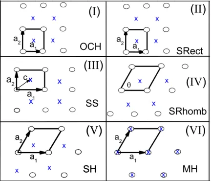
The ground state configurations were obtained numerically by comparing the total energy [Eq. (2.26)] of the 9-possible crystalline structures, described in Table 2.1 (for instance, see the structures in Fig. 2.1), for both⃗c = 0 (matching) and⃗c̸= 0 (staggered) cases as a function of λ and η. From all the considered structures the one with the lowest energy is chosen as the ground state configuration associated to the particular set of parameters (λ, η).
c (II) a 1 a 2 a 1 (III) (IV) SRhomb x x x x x x x x x x x x (I) a 2 OCH SS a 1 x x x x a 2 SRect a 1 x x x x (V) a 2 SH a 1 (V) a 2 SH a 1 x x x (VI) a 2 MH x x
x x x
x x
Figure 2.1: Top view of the structures of the ordered phases, where the circles (crosses) correspond to the lower (upper) layer. In the case of the matched phases, the layers are not displaced and are exactly on top of each other, as is shown for the MH phase.
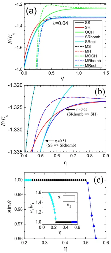
phase transitions, which can be observed more clearly in Fig. 2.2(b). For a first order structural phase transition, the energy is continuous but the first derivative of the energy with respect to η is discontinuous. In this case, the energy curves associated to different structures cross each other. For a second order transition, the energy and its first derivative are continuous, but the second derivative of the energy with respect to η is discontinuous. In this case, the energy curves merge with (or split away from) one another. The transition from the staggered rhombic (SRhomb) to the staggered hexagonal (SH) phase atη≈0.65 is an example of a first order structural transition, while a second order structural transition is observed when the system changes from the staggered square (SS) to the SRhomb phase. Notice that such phases differ from each other only in the aspect ratioa2/a1 and angleθ between the primitive vectors. As shown in Fig. 2.2(c) forη≈0.51
the system starts to change continuously from the SS (sinθ = 1; a2/a1 = 1 ) to the SRhomb phase
(sinθ ̸= 1).
0.2 0.3 0.4 0.5 0.6 0.96
0.97 0.98 0.99 1.00
0.0 0.2 0.4 0.6
1.0 1.2 1.4 1.6
si
n
(c)
a
1
a
2
a
2
]
a
1
0.4 0.5 0.6 0.7 0.8 0.9
-1.335 -1.330 -1.325 -1.320
(SRhomb => SH)
E
/
E
0
(b)
(SS => SRhomb)
0.0 0.5 1.0 1.5
-1.8 -1.6 -1.4 -1.2
SS
SH
OCH
SRhomb
SRect
MS
MH
MOCH
MRhomb
MRect
E
/
E
0
=0.04
(a)
Figure 2.2: (a) The total energy per particle (in units of E0 = Q2√n) as function of η for the
different phases presented in Table 2.1. (b) Detailed view of (a). (c) The sine of the angle between the primitive vectors ⃗a1 and⃗a2 of the SRhomb phase as a function of η. The inset in (c) shows
0.00 0.01 0.02 0.03 0.04 0.05
0.0 0.2 0.4 0.6 0.8 1.0
SH
S
R
h
o
m
b
SS MH
SRect
Figure 2.3: The zero temperature phase diagram where λ =µ2n/Q2 and η=d√
10 -3
10 -2
10 -1
10 0 10
-6 10
-5 10
-4 10
-3 10
-2 10
-1
~ 1.92 0.02
Figure 2.4: Thelog×log plot of the criticalλ(η) curve which separates the staggered phases from the MH phase taken from Fig. 2.3.
since the dipoles are all aligned along the z-axis and the inter-layer separation is zero. This is the well-known 2D Wigner crystal phase [34]. Along the λ = 0 line, the OCH phase is found only in a very small interval of η. In fact, already for η = 0.006 the OCH phase is no longer the ground state. The λ = 0 line corresponds to the case in which the inter-particle interaction is only electrostatic. In this case, the system can be found in five energetically favorable staggered configurations (phases I, II, III, IV, V - see Table 2.1) as a function ofη. The latter results are in complete agreement with those discussed earlier in Ref. [36].
which are not possible when only the magnetic dipole interaction is present.
The critical value of λ, where the system changes from a staggered (rectangular, square, rhom-bic, hexagonal) to the MH phase, is a monotonic increasing function of η. As seen in Fig. 2.3 we notice two distinct behaviors of λ(η). Initially, there is a fast increase of λ with increasing η, followed by an almost constantλ(η). Such a behavior can be qualitatively understood taking into account the range of the Coulomb and magnetic dipole inter-particle interaction. An inter-particle interaction is defined as short range if it decreases faster than 1/rα, whereα is the dimensionality
of the system [43]. In the opposite case, the interaction is long range. In this sense the Coulomb interaction can be considered as long range and the magnetic dipole interaction as short range. For small η the separation between layers is small and the dipole interaction is dominant over the electric interaction. As a consequence, the transition to the MH phase, which is the ground state for a system with only magnetic dipole interaction, occurs for small λ. For a large enough separation between the layers the coupling between dipoles in distinct layers (the inter-layer in-teraction) becomes very small. For example, forη= 0.8 the inter-layer interaction is only 0.3% of the total energy. As a consequence, for high enough values of η the layers become independent, and it becomes numerically impossible to determine if the SH or MH phase is the ground state. E.g., for η = 2.3 (λ≈ 0.044) the absolute difference in energy between the SH and MH phases is of the order of 10−8, which is the level of our numerical accuracy. In this case, the total energy is
twice the energy of each layer, since the particles in each layer barely interact.
A more detailed analysis of the critical λ(η) which defines the transition from a staggered to the MH phase identifies a clear crossover between the fast (strong coupling between dipoles in distinct layers) and slow increase of λ(η). This is shown in Fig. 2.4, where a log×log plot of the critical λ(η) curve which separates the staggered phases from the MH phase is presented. As can be seen, there is a power law increase of λ(η) for η . 0.15 with exponent β ∼ 1.92. Thus for η .0.2, the critical distance between the layers scales as d ∝(µ/Q)1.04n0.021, which indicates
a weak dependence on the density and an almost linear dependence on the ratio µ/Q. This scaling behavior can be understood as follows: the interlayer dipole interaction ∼ µ2/d3 while
the Coulomb interlayer interaction ∼ Q2/d and therefore we expect the staggered to matched
transition approximately when Q2/d∼µ2/d3 and thus λ∼η.
To conclude, we also present a hatched area in the (λ, η) phase diagram (Fig. 2.3). It cor-responds to a disordered phase which can not be obtained from our analytical calculations. The discussions concerning such a phase will be postponed to the next section.
2.4
Dynamical Properties
The phonon spectra are calculated within the harmonic approximation. The phonon frequencies for a general lattice are directly obtained from the dynamical matrix through the square root of the eigenvalues. Since we are studying a 2D crystal with two particles per unit cell (one in each layer), the dynamical matrix corresponds to a 4×4 matrix which can be written as
D=
(
DAA DAB
DBA DBB
)
, (2.27)
where DAA, DAB, DBA, DBB are 2×2 block matrices which include the intra- and inter-layer
electric and magnetic interactions. The labels A and B describe the distinct layers, and each block matrix is of the form
[Dτ ν(⃗q)]αβ = [Dτ νel(⃗q)]αβ + [Dτ νmag(⃗q)]αβ, (2.28)
where τ, ν =A, B; α, β =x, y. Following the procedure described in Ref. [36] and by using Eqs. (2.12a), (2.12b), (2.19a), and (2.19b), the different terms present in Eq. (2.28) are given by
[DAAel (⃗q)]αβ =
1 m{[S
AA
el (0)]αβ+ [SelAB(0)]αβ
−[SelAA(⃗q)]αβ},
(2.29a)
[DABel (⃗q)]αβ =
1 m{−[S
AB
el (⃗q)]αβ}, (2.29b)
[DAAmag(⃗q)]αβ =
1 m{[S
AA
mag(0)]αβ+ [SmagAB(0)]αβ
−[SmagAA (⃗q)]αβ},
(2.29c)
[DAB
mag(⃗q)]αβ =
1 m{−[S
AB
mag(⃗q)]αβ}, (2.29d)
where m is the mass of each particle and
[SelAA(⃗q)]αβ =−Q2lim
r→0∂α∂βT0(⃗r, ⃗q)
=−Q2√ns[E(⃗q)]αβ ,
(2.30a)
[SAB
el (⃗q)]αβ =−Q2lim
r→0∂α∂βTI(⃗r, ⃗q)
=−Q2√ns[F(⃗q, η)]αβ ,
(2.30b)
[SmagAA(⃗q)]αβ =−µ2lim
r→0∂α∂βψ0(⃗r, ⃗q)
=−µ2√ns[G(⃗q)]αβ ,
[SmagAB(⃗q)]αβ =−µ2lim
r→0∂α∂βψI(⃗r, ⃗q)
=−µ2√ns[H(⃗q, η)]αβ .
(2.30d)
The auxiliary functions [E(⃗q)]αβ, [F(⃗q, η)]αβ, [G(⃗q)]αβ, and [H(⃗q, η)]αβ are given by:
[E(⃗q)]αβ =−
∑
⃗ G
(⃗q+G)⃗ α(⃗q+G)⃗ βΦ
(
|⃗q+G⃗|2
4πns
)
+ lim
r→0
∑
⃗ R̸=⃗0
e−i⃗q·R⃗∂α∂βΦ
(
πns|⃗r−R⃗|2
)
+δαβ
4 3πns,
(2.31a)
[F(⃗q, η)]αβ =−
∑
⃗ G
(⃗q+G)⃗ α(⃗q+G)⃗ β
×e−i ⃗G·⃗cΨ
(
|⃗q+G⃗|2
4πns
, πη2
)
+ lim
r→0
∑
⃗ R
e−i⃗q·(R⃗−⃗c)
×∂α∂βΦ
(
π[ns|⃗r−R⃗ +⃗c|2+η2]
)
,
(2.31b)
[G(⃗q)]αβ =−πns
∑
⃗ G
(⃗q+G)⃗ α(⃗q+G)⃗ βΥ
(
|⃗q+G⃗| 2ε ,0
)
+ lim
r→0
∑
⃗ R̸=⃗0
e−i⃗q·R⃗∂α∂βΩ1
(
|⃗r+R⃗|)+δαβ
8ε5
5√π,
(2.31c)
[H(⃗q, η)]αβ =−πns
∑
⃗ G
(⃗q+G)⃗ α(⃗q+G)⃗ β
×ei ⃗G·⃗cΥ
(
|⃗q+G⃗| 2ε , εd
)
+ lim
r→0
∑
⃗ R
e−i⃗q·(R⃗+⃗c)∂α∂βΩ2
(
|⃗r+R⃗ +⃗c|),
(2.31d)
and the functions Υ(x, y), Ω1(x), and Ω2(x) which appear in Eqs. (2.31c) and (2.31d) are:
Υ(x, y) = √4ε πe
−x2
−y2
+∑
±
0 1 2 3
M X
X M
(a)
0 1 2 3
M X
(b)
Ω1(x) =
erfc(εx) x3 +
2εe−ε2x2
√
πx2 , (2.32b)
Ω2(x) =
erfc(εx) x3 +
2εe−ε2
x2
√
πx2
−3d2
[
erfc(εx) x5 +
2ε(3 + 2ε2x2)e−ε2
x2
3√πx4
]
.
(2.32c)
By using the relations ε = 1/r0 =√πns, ns =n/2, and λ =µ2n/Q2 the terms of the matrix
given in (2.27) become
[DAA(⃗q)]αβ = −
Q2n3/2
m
[
1 23/2n
s{
[E(0)]αβ + [F(0, η)]αβ
−[E(⃗q)]αβ}+
λ (2ns)5/2{
[G(0)]αβ
+ [H(0, η)]αβ−[G(⃗q)]αβ}] ,
[DAB(⃗q)] αβ =
Q2n3/2
m
[
1 23/2n
s
[F(⃗q, η)]αβ
+ λ
(2ns)5/2
[H(⃗q, η)]αβ
]
.
The two layers of particles are equivalent. In this case, DAA =DBB, DAB = [DBA]†, and the
dynamical matrixDmay now be calculated as a function of λ,⃗q, andη. In general, the dynamical matrix is complex hermitian. Therefore, it is possible to apply an unitary transformation in order to generate a real and symmetric matrix. Such a transformation is given by the matrix
U = √1
2
(
I2 iI2
iI2 I2
)
(2.33)
where I2 is the 2×2 identity matrix, and
¯
D=U DU−1 =
(
DAA+ ImDAB ReDAB
ReDAB DAA−ImDAB
)
(2.34)
where ReDAB and ImDAB are the real and imaginary parts ofDAB, respectively. Since a unitary
transformation does not change the eigenvalues, we may consider now the real and symmetric matrix ¯D in order to obtain the eigenvalues and the phonon frequencies. For each (λ,η), which specify a given structure in the phase diagram shown in Fig. 2.3, we vary the wave vector⃗qalong a given symmetry direction of the first Brillouin zone of the corresponding phases. For each value of ⃗q, we generate a 4×4 matrix which gives us four eigenvalues ω2
0 1 2 137.1580 137.1585 137.1590
X
J
0.8 0.1
X
J
Figure 2.6: The phonon spectrum for the MH phase for different values of η and fixed λ. The high-symmetry directions of the reciprocal space are presented in the inset.
ω2
0 = Q2n3/2/m, and for each eigenvalue a corresponding eigenvector ⃗e(⃗q, j) which indicates the
direction of the phonon oscillation.
In our analysis of the dispersion relation we will present only frequencies which are real positive, i. e. ω2
j(⃗q)/ω20 ≥0. Forω2 <0, the frequencies are imaginary, which means that the amplitudes of
particle oscillation become an exponentially increasing function of time. In this case, the crystalline structure is unstable and will not exist. As commented earlier, in all phases studied in the previous section there are two particles per unit cell, one in each layer. As a consequence, there are two acoustic and optical modes which are associated to the in-phase and out-of-phase vibrations of particles in the unit cell, respectively. The acoustic branch is characterized byω(⃗q)→0 for⃗q→0, while in the optical branch ω(⃗q)→constant in the limit ⃗q→0. Besides, the acoustic and optical branches may also be defined as longitudinal, ⃗e ∥ ⃗q, and transverse modes [44], ⃗e ⊥ ⃗q. Due to the extended parameter space, we present here only some examples which illustrate the general behavior of the phonon spectrum.
high-0.0 0.5 1.0 1.5 2.0 0.4
0.6 0.8 1.0
v
T
A
/
v
0
J
X
Figure 2.7: The sound velocity (in units of v0 = ω0/√n) of the TA mode as a function of η for
λ= 0.046 and λ= 0.5.
symmetry points in the first Brillouin zone are indicated in the insets. Notice that for both values of λ, which are one order of magnitude distinct, the same qualitative behavior is found for the phonon frequencies as a function of the wave vector. The phonons soften with increasing η along the ΓX direction. Along the XM direction, the normal mode frequencies are degenerate for any value of η. The lowest normal mode frequencies cross at a specific q-value which is independent of η. Notice that in the ΓM direction the lowest energy phonons soften with decreasing η which is the opposite behavior found along the ΓX direction.
For the MH phase, we present in Fig. 2.6, the phonon spectrum for λ = 0.046. In this case, the bilayer system is found in the MH phase for any value of η. Again the high-symmetry points in the reciprocal space are labelled in the inset. For a fixed density n, the parameter η=d√n/2 is directly related to the separation between the layers. For η = 0.1, a large gap between the acoustic and optical modes is observed. The later ones, which describe the out-of-phase vibrations of particles in distinct layers, are two orders of magnitude larger than the acoustic ones. Such a behavior is due to the strong dipolar magnetic interaction for small η. Notice that the dipole interaction (∝ 1/r3) is dominant over the Coulomb interaction (∝ 1/r) for short distances r.
layers. This is in agreement with the comment made in the previous section that, for η = 0.8 the inter-layer interaction is only 0.3% of the total energy. The gap between the acoustic and optical modes is observed for η . 0.44. For η >> 1 the acoustic and optical modes (transverse and longitudinal) become degenerate since the coupling between the layers becomes very small, and the system behaves as two independent single layer systems.
As shown previously for the SS phase, we also find a monotonic behavior of the phonon spectrum of the MH phase for λ = 0.046, i.e. there is a softening of the phonon frequencies with increasing η for all the high-symmetry directions of the reciprocal space. Such a behavior is interesting, since in the bilayer system with only dipole interaction, a non-monotonic behavior of the phonon spectrum was observed as a function ofη [37]. Such a behavior was explained in Ref. [37] as being linked to the competitive character of the dipole-dipole interaction. In that case, the non-monotonic behavior of the phonon spectrum also revealed a non-monotonic dependence of the sound velocity onη. In addition, for η→0 the sound velocity is a factor √2 larger than the value obtained for η >> 1, showing that for small separations the bilayer system of dipoles behaves as a crystal of particles with twice larger dipole moment and mass. In the present bilayer system of charged dipole particles, we found that such a non-monotonic behavior for the phonon spectrum depends on the parameterλas shown in Fig. 2.7. Forλ = 0.046 the sound velocity is a monotonic function of η, but e.g. for λ = 0.5 it is non-monotonic exhibiting a minimum for η = 0.73. We found that the non-monotonic versus monotonic behavior of the sound velocity is associated to a change in the attractive/repulsive character of the total energy, i.e. it is attractive when vT A is
non-monotonic. This is an interesting feature, since e. g. in electrically steric colloidal systems the charge adsorbed on the colloidal particles can be controlled, for example, by changing the PH of the solution [10]. In addition, since the melting temperature can in principle be calculated from the normal mode frequencies, the non-monotonic behavior of the phonon spectrum should play an important role in the behavior of the melting temperature, which should become noticeable when varyingλ.
0.0 0.5 1.0 1.5 2.0 2.5
X J
MH SH
X
J
Figure 2.8: The phonon spectrum for the SH and MH phase for differentλand fixedη= 0.8. The high-symmetry direction of the reciprocal space are presented in the inset.
from the SH to the MH phase.
Now we study the interval of stability of the different phases (deduced from the phonon spec-trum) and compare it with the position of the phase boundary (obtained from the minimum energy criterion).
As expected, not only the phase boundary but also the stability of the MH phase is enhanced with increasingλin the sense that the interval ofηfor which the MH phase is stable, increases with increasing λ. This is shown in Fig. 2.9 for λ = 0.01 and 0.03. Notice that the stability interval of the MH phase is larger than the phase boundaries in both cases, indicating that the MH phase is metastable beyond the phase boundary. In such a case, the structural phase transition is first order. The interval of stability of the staggered phases with increasingλdepends on the crystalline structure. For the OCH, which is not found as a ground state for λ ̸= 0, the interval of stability decreases with increasingλ (Fig. 2.9). For the SS phase and λ= 0.03, the interval of stability of the SS phase (0.238 . η . 0.534) becomes larger than its phase boundary (0.262 . η . 0.534) and a first order transition separates the SS and MH phases. When the SS phase is bordered by the SRect and SRhomb phases (λ . 0.027) its phase boundary and interval of stability coincide and these phases are separated by a second order structural (continuous) transition, characterized by the softening of one of the phonon mode frequencies. The SRect phase, which is suppressed as a ground state configuration for λ &0.027, is still stable as shown e. g. for λ= 0.03.
0.0 0.4 0.8 0.0 0.4 0.8
0.0 0.5 1.0 1.5 2.0 2.5 3.0 0.0
0.2 0.4 0.6 0.0 0.2 0.4 0.6
New Phase
g
(
r
)
T=0
SH Phase New Phase
SH Phase
T=1x10
-5
g
(
r
)
=0.03 =0.8
T=0
g
(
r
)
r T=3x10
-6
(a)
(b)
(c)
(d)
g
(
r
)
Figure 2.10: The radial distribution function as calculated from our MC simulations for the new phase and the SH phase for two different temperatures. For the new phase: (a) T = 1×10⁻⁵
and (b) T = 0. For the SH phase: (c) T = 0 and (d) T = 3×10⁻⁶. The configuration of the
can be stable for some interval of η. For instance, for η = 0.24 (λ = 0.03) the MH, SS and OCH phases are all stable. In contrast, for the pure Coulomb [36] and magnetic [37] systems a maximum number of two phases were found to be stable in a given interval of η. The presence of many stable phases might have important consequences for the melting temperature. In this case, structural transitions between such phases should, in principle, be possible before the system melts.
From Fig. 2.9, we see that in the largeη-region (hatched) in the (λ, η) phase diagram (Fig. 2.3) there is a discrepancy between the found lowest energy structure and its stability. For λ = 0.01 we found that the SH configuration has the lowest energy for η > 0.706 while it is only stable for η > 0.727. For η < 0.727 the frequency of the transverse acoustic mode of the SH phase becomes imaginary along the ΓX and ΓJ directions. Imaginary frequency is also found for the other phases presented in Table 2.1. From this observation we are forced to conclude that in the region 0.706 < η < 0.727 none of the 9 crystal structures can be the ground state. This discrepancy is even more pronounced for λ = 0.03 where the SH phase was found to be unstable in the range 0.660< η < 0.981 where (from the analytical calculations) it was initially predicted to be the ground state (Fig. 2.3). An important lesson to be learned from this stability analysis is that one has to be very careful to rely only on the most plausible crystal structures in combination with an energy minimization when deciding which phase is the ground state. In order to find the true ground state in this area of the phase diagram we resorted to a pure numerical approach.
We used Monte Carlo (MC) numerical simulations in order to find the stable ground state configuration. As an example we took λ= 0.03 and η= 0.8 and we notice from the inset of Fig. 2.10(a) that the obtained ground state configuration is similar to the SH phase (inset Fig. 2.10(c)), but the 2D displacement of one layer with respect to the other is different, i. e. ⃗c̸= (⃗a1+⃗a2)/3.
The energy of this new phase is slightly lower, i.e. the difference with the SH phase is ∆E ≈10−5.
To test numerically the stability of the new configuration (inset of Fig. 2.10(a)) we compare the T = 0 and T ̸= 0 pair distribution functions g(r) calculated from the MC simulations. See that g(r) contains both the inter-layer (g12(r)) and the intra-layer (gii(r)) radial distribution,
where the latter takes into account only the inplane component. As can be observed from Fig. 2.10(a) the g(r) function remains almost unaltered when we increase T slightly, indicating the thermal stability of the phase. That the SH phase is indeed unstable we tested by using our MC simulations and let the program run forT ̸= 0. Notice that theg(r) forT = 0 and the one for very low temperature T = 3×10⁻⁶ are different (Figs. 2.10(c) and (d)). There is a clear disordering
of the lattice which indicates that very small thermal fluctuations destroy already the SH phase and consequently the SH phase is indeed unstable.
1.32 1.34 1.36 1.38 2.65 2.70 2.75 0
20 40 60 80
SH
new phase
g
i
i
(
r
)
r
=0.03 0.8
two peaks reflect only the short range inter-layer ordering. In fact, a more careful analysis reveals that the new phase does not consists of a perfect hexagonal configuration in each layer. This can be seen in Fig. 2.11 where a comparison between the pair distribution functions gii(r) calculated
in each layer of the new phase and the one calculated in each layer of the SH phase is presented in two narrow ranges of r. The difference observed in the gii(r) functions between both phases
indicates that the new phase does not consist of a perfect hexagonal lattice in each layer. Notice that for each peak of the SH phase, there appear many peaks (or a broadening of the hexagonal lattice peak) of the new phase around it, which indicates that the lattice is distorted (or strained).
2.5
Conclusions
We studied a 2D classical bilayer system of charged magnetic dipoles. The phase diagram at T = 0, as well as the phonon spectra were obtained through minimization of the energy and within the harmonic approximation, respectively. We obtained a very rich phase diagram at T = 0 with six different crystalline structures, being five staggered phases (OCH, SS, SRect, SRhomb, SH), which were previously found as the ground state configuration when no magnetic interaction is present [36], and a MH phase, which was obtained as the only ground state configuration for the bilayer system of dipoles aligned perpendicularly to the layers [37]. Notice that the presence of both Coulomb and magnetic interaction allows the appearance of phases which were not found in the pure Coulomb (MH phase) and magnetic systems (staggered phases). In the latter, the charges on the dipole particles allow the bilayer system to crystallize in different lattice structures which are not possible when only the magnetic dipole interaction is present, e.g. the SH and SRhomb phases appear not stable for any interval of η. The phase diagram was obtained as a function of the separation between the layers (η), and a parameter (λ) which is associated to the relative strength of the magnetic and Coulomb interaction between the particles. We found that the staggered phase boundaries depend on λ, e.g., the SRect phase is no longer the ground state
for λ&0.027.
velocity behavior. Notice that in electrically steric colloidal systems the charge adsorbed on the colloidal particles can be controlled, for example, by changing the pH of the solution [10]. In this case, for a large enough separation between the layers, where only the MH and SH phases are found as ground state, it is possible to tune the configuration between staggered and matching by changing e.g. the charge on the particles (fixed µ) and, consequently, λ. Alternatively we may change the magnetic field strength in order to tune the value of λ. In addition, since the melting temperature can, in principle, be calculated from the normal mode frequencies (at least within the harmonic approximation), the non-monotonic behavior of the phonon spectrum might play an important role when determining the melting temperature for different λ.
The stability of the phases obtained from the phonon spectrum were compared with the phase boundaries for different values of (λ, η). In particular, the MH phase is enhanced with increasing λ, in the sense that a larger phase boundary and interval of stability is observed. The SRect phase, which is no longer observed as ground state configuration for λ & 0.027 still appears as a metastable configuration. As an important finding, the presence of both electric and magnetic interaction stabilizes up to three phases in some η-interval of a given ground state configuration, and this fact should have profound implications on the melting temperature, since structural transitions may take place for temperatures T ̸= 0.
We found a region in the (λ, η) phase diagram where the SH phase has the lowest energy among the considered 9 crystal structures while from the phonon spectrum it appears to be unstable. Monte Carlo simulations were used to determine the ordered structure in this region, and we found that the lowest energy configuration corresponds to a distorted hexagonal lattice structure.