Imaging tropical peatlands in Indonesia using ground penetrating radar (GPR) and electrical resistivity imaging (ERI): implications for carbon stock estimates and peat soil characterization

(1)

BGD

12, 191–229, 2015

C stock estimates and peat soil

X. Comas et al.

Title Page

Abstract Introduction

Conclusions References

Tables Figures

◭ ◮

Back Close

Full Screen / Esc

Printer-friendly Version Interactive Discussion

Discussion

P

a

per

|

Discussion

P

a

per

|

Discussion

P

a

per

|

Discussion

P

a

per

|

Biogeosciences Discuss., 12, 191–229, 2015 www.biogeosciences-discuss.net/12/191/2015/ doi:10.5194/bgd-12-191-2015

This discussion paper is/has been under review for the journal Biogeosciences (BG). Please refer to the corresponding final paper in BG if available.

Imaging tropical peatlands in Indonesia

using ground penetrating radar (GPR) and

electrical resistivity imaging (ERI):

implications for carbon stock estimates

and peat soil characterization

X. Comas1, N. Terry2, L. Slater2, M. Warren3, R. Kolka4, A. Kristijono5, N. Sudiana5, D. Nurjaman5, and T. Darusman6

1

Department of Geosciences, Florida Atlantic University, Davie, FL 33314, USA

2

Department of Earth & Environmental Sciences, Rutgers-Newark, Newark, NJ 07102, USA

3

USDA Forest Service, Northern Research Station, Durham, NH 03824, USA

4

USDA Forest Service, Northern Research Station, Grand Rapids, MN 55744, USA

5

Indonesian Agency for Assessment and Application of Technology (BPPT), Jakarta 10340, Indonesia

6

(2)

BGD

12, 191–229, 2015

X. Comas et al.

Title Page

Tables Figures

◭ ◮

Back Close

Full Screen / Esc

Discussion

P

a

per

|

Discussion

P

a

per

|

Discussion

P

a

per

|

Discussion

P

a

per

|

Received: 21 September 2014 – Accepted: 6 December 2014 – Published: 6 January 2015

Correspondence to: X. Comas ([email protected])

(3)

BGD

12, 191–229, 2015

X. Comas et al.

Title Page

Tables Figures

◭ ◮

Back Close

Full Screen / Esc

Discussion

P

a

per

|

Discussion

P

a

per

|

Discussion

P

a

per

|

Discussion

P

a

per

|

Abstract

Current estimates of carbon (C) storage in peatland systems worldwide indicate trop-ical peatlands comprise about 15 % of the global peat carbon pool. Such estimates are uncertain due to data gaps regarding organic peat soil thickness and C content. Indonesian peatlands are considered the largest pool of tropical peat carbon (C),

ac-5

counting for an estimated 65 % of all tropical peat while being the largest source of carbon dioxide emissions from degrading peat worldwide, posing a major concern re-garding long-term sources of greenhouse gases to the atmosphere. We combined a set of indirect geophysical methods (ground penetrating radar, GPR, and electrical resis-tivity imaging, ERI) with direct observations from core samples (including C analysis) to

10

better understand peatland thickness in West Kalimantan (Indonesia) and determine how geophysical imaging may enhance traditional coring methods for estimating C storage in peatland systems. Peatland thicknesses estimated from GPR and ERI and confirmed by coring indicated variation by less than 3 % even for small peat-mineral soil interface gradients (i.e. below 0.02◦). The geophysical data also provide

informa-15

tion on peat matrix attributes such as thickness of organomineral horizons between peat and underlying substrate, the presence of wood layers, buttressed trees and soil type. These attributes could further constrain quantification of C content and aid re-sponsible peatland management in Indonesia.

1 Introduction

20

Globally, tropical peatlands are estimated to store 89 Pg C, equivalent to about one-tenth of the current atmospheric carbon pool (Page et al., 2011). Indonesia contains about 47 % of the World’s tropical peatlands, with an estimated 21 Mha (Wahyunto et al., 2003, 2004; Page et al., 2011). Indonesian peat swamps have been globally significant carbon sinks over the past 15 000 years, and currently contain 65 % of total

25

(4)

BGD

12, 191–229, 2015

X. Comas et al.

Title Page

Tables Figures

◭ ◮

Back Close

Full Screen / Esc

Discussion

P

a

per

|

Discussion

P

a

per

|

Discussion

P

a

per

|

Discussion

P

a

per

|

in peat soils has focused on boreal and arctic regions, many uncertainties exist re-garding the role of tropical peat soils as a significant component of the global carbon cycle and their dynamics under a changing climate. Peatlands are also well known for other ecological functions such as regulating water supply and biodiversity conserva-tion (Menke, 1989,Červen´y and Soares, 1992; Geuzaine and Remacle, 2009;

Robin-5

son et al., 2013). Once significant carbon sinks, vast areas of Indonesian peatlands are becoming large, long-term sources of greenhouse gases (primarily carbon dioxide, CO2) to the atmosphere due to deforestation, drainage and/or peat fires (Kruse, 2013).

When peat is drained, available oxygen stimulates microbial activity and organic mat-ter decomposition. In addition, drained peat is highly vulnerable to fire and large areas

10

of degraded Indonesian peatlands burn each year producing large scale CO₂ emis-sions and air pollution (van Schoor, 2002; Ahmed and Carpenter, 2003). Increased heterotrophic respiration and peat burning emits significant amounts of CO2to the

at-mosphere, contributing to global warming and climate change. In a recent overview of carbon distribution based on a 2008 inventory, Indonesia was considered the largest

15

source of CO2emissions from degrading peat worldwide, with values exceeding other

large producers such as China and the United States by almost one order of mag-nitude (Joosten, 2009). Furthermore, emissions of other greenhouse gases (such as nitrous oxide, N2O and methane, CH4) may also be enhanced in peat soils by the

addition of fertilizers or rewetting of drained peatlands. For all these reasons,

Indone-20

sia’s peatlands are considered “hot spots” for greenhouse gas emissions, ecosystem services and biodiversity, and are therefore targeted as priority areas for climate miti-gation strategies including programs such as Reducing Emissions from Deforestation and Forest Degradation (or REDD+). However, the lack of information on area, depth and volume of Indonesian peatlands contributes to large uncertainties in patterns of

25

peat carbon pools and fluxes, contributing to management decisions which exacerbate greenhouse emissions from peatland degradation.

(5)

high-BGD

12, 191–229, 2015

X. Comas et al.

Title Page

Tables Figures

◭ ◮

Back Close

Full Screen / Esc

Discussion

P

a

per

|

Discussion

P

a

per

|

Discussion

P

a

per

|

Discussion

P

a

per

|

est range of uncertainty in terms of C storage, mainly due to the uncertainties in peat thickness and C content, and because few attempts have been made to estimate trop-ical peatland carbon (C) stores at local to global scales. Page et al. (2011) reported between 82 and 92 Pg C is stored in tropical peatlands worldwide, comprising about 15 % of the global peat carbon pool. According to the same study, Indonesian

peat-5

lands store about 57 Pg C. Yu et al. (2010) estimated that tropical systems cover a to-tal area of 368 500 km2and represent 44–55 Pg C. These peats accumulated at rapid rates between 8000–4000 years ago to present (Yu et al., 2010). Estimating peat car-bon storage requires accurate volume measurements calculated from peat area and thickness. Page et al. (2011) calculated peat volume for Indonesia using a mean peat

10

depth of 5.5 m, which was based on very few geographically biased data consider-ing the scale at which the mean depth estimate was applied: 206 950 km2 through-out Indonesian Borneo (Kalimantan), Sumatra and Papua. Perhaps the most accurate peat volume measurements published at a local scale in Indonesia were reported by Jaenicke et al. (2008) who modeled peat depth using a combination of 542 discrete

15

field measurements from direct coring, surface elevation models, satellite imagery and spatial interpolation across four peat domes in Central Kalimantan. Despite the large number of direct measurements of peat thickness, the uncertainty in carbon storage estimates ranged from 13–25 %, which the authors attributed to bedrock unconformi-ties not considered in the models of peat volume derived from relationships between

20

surface elevation and peat thickness (Jaenicke et al., 2008). Most current eﬀorts to model peat depth are based on the assumption that peat deposits occur in uniform biconvex formations, despite evidence from field measurements indicating consider-able buried topography under the peat in some areas such as riverbeds and levees. For example, surveys have shown mineral substrate topography changing as much as

25

3 m within single transects (of less than one km) across several peat domes in Borneo (Dommain et al., 2010, after Konsultant, 1998).

(6)

re-BGD

12, 191–229, 2015

X. Comas et al.

Title Page

Tables Figures

◭ ◮

Back Close

Full Screen / Esc

Discussion

P

a

per

|

Discussion

P

a

per

|

Discussion

P

a

per

|

Discussion

P

a

per

|

lated to peatland development and stratigraphy including: peat thickness characteri-zation (Worfield et al., 1986; Warner et al., 1990); the presence of natural soil pipes (Holden et al., 2002) and pipelines in peat (Jol and Smith, 1995); hydrogeology and pool formation in peatlands (Slater and Reeve, 2002; Comas et al., 2005b, 2011b; Ket-tridge et al., 2008); geoelectrical properties of the peat matrix (Theimer et al., 1994;

Co-5

mas and Slater, 2004); peatland evolution (Comas et al., 2004; Kettridge et al., 2012); and biogenic gas distribution and dynamics in peat (Comas et al., 2005a, 2007, 2008, 2011a; Parsekian et al., 2010, 2011). The pore waters of peat soils in ombrotrophic boreal peatlands (typically being 200 µS cm−1

or less) are characterized by low fluid electrical conductivity, resulting in GPR investigation depths of up to 11 m (Slater and

10

Reeve, 2002). Electrical resistivity imaging (ERI) has also been used in boreal systems for investigating peatland stratigraphy (Meyer, 1989) and hydrogeology (Slater and Reeve, 2002), peatland evolution (Comas et al., 2004, 2011b; Kettridge et al., 2008) and biogenic gas distribution and dynamics in peat soils (Slater et al., 2007). Electrical conductivity of peat typically increases with depth in boreal systems due to increased

15

dissolved ion concentration and the underlying mineral soil usually exhibits a strong electrical contrast to the terrestrial peat (Slater and Reeve, 2002). Such observations support the use of GPR and ERI methods for mapping tropical peatlands, although diﬀerences in peat types, terrain and/or vegetation cover between boreal and tropical systems must be considered.

20

To our knowledge, we report the first study using a combination of GPR and ERI to better characterize peatland systems in the tropics. The objectives of this study were to (1) estimate peat thickness in a non-invasive and spatially continuous way at a resolution previously unreported for tropical peatlands; and (2) evaluate whether information on geological settings and/or peat composition (related to carbon content)

25

(7)

BGD

12, 191–229, 2015

X. Comas et al.

Title Page

Tables Figures

◭ ◮

Back Close

Full Screen / Esc

Discussion

P

a

per

|

Discussion

P

a

per

|

Discussion

P

a

per

|

Discussion

P

a

per

|

than those derived from traditional coring methods. Advancing in this knowledge could potentially aid responsible peatland management in Indonesia.

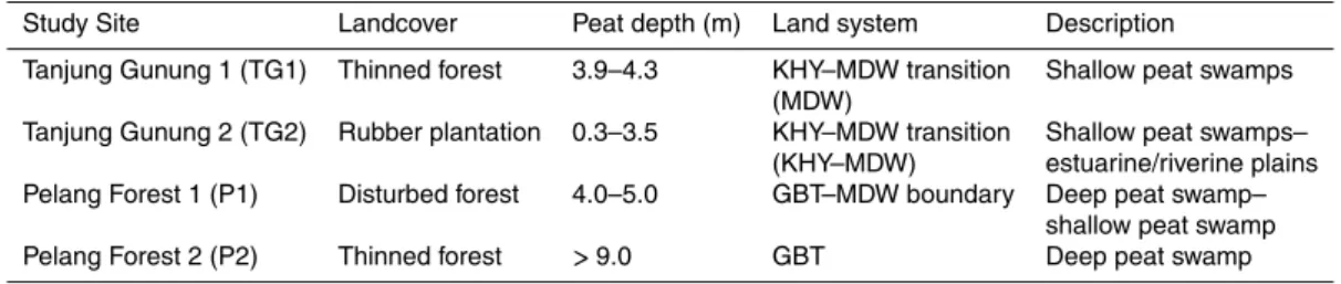
2 Field sites

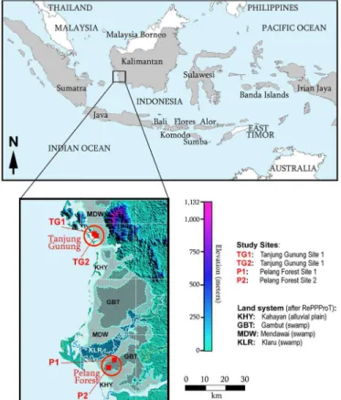
Two peatland sites located in the West Kalimantan Province were chosen for this study: Tanjung Gunung (Sejahtera village, Kayong Utara District); and Pelang (Pelang village,

5

Ketapang District). Both sites had been previously visited by investigated by USFS (United States Forest Service) collaborators and were known to contain variable peat thickness and multiple landcover types, while providing relatively easy access. The Tan-jung Gunung site (hereafter referred to as TG) is adjacent to Gunung Palung National Park and its natural resources have been heavily exploited by the local community for

10

decades. Within the TG site, two areas along the same peat formation were studied: a thinned, degraded forest (TG1) and a mature rubber plantation which is located at the edge of the peat formation (TG2). The physiographic terrain at TG is a 6 km wide swamp peatland known as Mendawai, MDW (RePPProT, Regional Physical Planning Programme for Transmigration, 1990) that is characterized by shallow peat. Kahayan

15

(KHY) peaty alluvial plains are also formed along the seaward edges of MDW (inset in Fig. 1). Although the two selected study sites (TG1 and TG2) are only approximately 1 km apart and are both situated in a transition zone between KHY and MDW ecosys-tems, diﬀerences exist in terms of thickness of peat and organomineral transitional layers and water table depth. While TG1 is characterized by MDW properties (i.e.

shal-20

low peat swamps), TG2 is characterized by a mixture of MDW and KHY properties, including landforms such as coalescent estuarine and riverine plains with lithologies that include alluvium and marine sediments.

At the Pelang forest site (hereafter referred to as P), two areas along the same peat formation were also studied: a thinned, degraded forest occurring on approximately

25

(8)

BGD

12, 191–229, 2015

X. Comas et al.

Title Page

Tables Figures

◭ ◮

Back Close

Full Screen / Esc

Discussion

P

a

per

|

Discussion

P

a

per

|

Discussion

P

a

per

|

Discussion

P

a

per

|

very deep peat (>9 m). Compared to the Tanjung Gunung sites (TG1 and TG2), Pelang

Forest sites are characterized by extensive peatlands over about 20 km×20 km (inset in

Fig. 1), forming three types of peat ecosystems: (a) Klaru (KLR) or permanently water logged peaty floodplains, (b) Gambut (GBT) or deeper dome-shaped peat swamp; and (c) Mendawai (MDW) or shallower peat swamp. Similar to the previous sites at TG,

5

Kahayan (KHY) peaty alluvial plains are also formed along the seaward edges of MDW (Fig. 1). Two measurement sites were also selected at this location and included P1 (located at a boundary zone of GBT and MDW), whereas site P2 is located within GBT. The results of 2-D resistivity measurements described below show significant diﬀerences in these two ecosystems. Additional specifications for each study site are

10

summarized in Table 1, including a description of the landcover, average peat depth. and land system after RePPProT (1990).

3 Methods

3.1 Ground penetrating radar

Ground penetrating radar (GPR) is a fast, reliable, and inexpensive geophysical method

15

for non-destructive mapping of shallow subsurface features in peatlands at scales rang-ing from kilometers for geological features influencrang-ing peatland hydrology such as es-kers (Comas et al., 2011b), to centimeters for determination of bubble distribution in peat blocks at the laboratory scale (Comas and Slater, 2007). The GPR technique in-volves the transmission of short pulses of high frequency electromagnetic (EM) energy

20

into the ground, and measurement of the energy reflected from interfaces between subsurface materials with contrasting electrical properties. In the most common de-ployment, one antenna (the transmitter) radiates short pulses of EM waves, and the other antenna (the receiver) measures the reflected signal as a function of time. Re-flections are primarily caused by changes in water content, which in turn are

deter-25

(9)

BGD

12, 191–229, 2015

X. Comas et al.

Title Page

Tables Figures

◭ ◮

Back Close

Full Screen / Esc

Discussion

P

a

per

|

Discussion

P

a

per

|

Discussion

P

a

per

|

Discussion

P

a

per

|

primarily controlled by relative dielectric permittivityε_r(b), are required to convert the

EM wave travel times recorded by GPR to depths of significant reflectors. Due to the high water content of peat soils,ε_r(b) _{of peat is very high compared to inorganic}

min-eral soils, being 50–70 depending on peat type. Whenε_r(b)is generally well constrained

from velocity analysis, estimation of peat depth is typically accurate to within∼20 cm

5

(Parsekian et al., 2012).

GPR surveys were performed using a Mala-RAMAC system with 100, 200 and 50 MHz antennas, with the 100 MHz antennas proving the best compromise between depth of investigation and resolution. Malfunctioning of the 50 MHz antennas towards the end of the campaign prevented testing depth of penetration for this frequency at

10

study sites with thicker peat columns. The spacing between traces was 0.2 m and 16 stacks (or replicates) were used for each trace. Two types of surface GPR surveys were performed: (1) common oﬀset surveys, where both transmitter and receiver antennas are kept at a constant distance as they are moved along transects; and (2) common mid-point (CMP) measurements where transmitter and receiver are separated

incre-15

mentally to larger distances. While common oﬀset surveys are frequently used for sub-surface imaging purposes (since profiles resemble a geological cross-section where depth is expressed as a travel time of the EM wave), CMPs are used for velocity esti-mation.

ERI is a method for generating images of the variation in electrical resistivity in either

20

2 or 3 dimensions below a line or grid of electrodes placed at the Earth’s surface. Data are acquired by measuring the voltage diﬀerences between electrode pairs in response to current injection between additional electrode pairs. Numerical methods are used to solve the Poisson equation relating the theoretical voltages at the electrodes to the distribution of resistivity in the subsurface. Inverse methods are used to find a model

25

(10)

BGD

12, 191–229, 2015

X. Comas et al.

Title Page

Tables Figures

◭ ◮

Back Close

Full Screen / Esc

Discussion

P

a

per

|

Discussion

P

a

per

|

Discussion

P

a

per

|

Discussion

P

a

per

|

controlled by water content, chemical composition of the pore water and soil surface area/grain size distribution.

3.2 Electrical resistivity imaging

Electrical resistivity imaging was conducted using a four electrode Wenner configu-ration with both 1 and 2 m electrode spacing and providing maximum imaged depths

5

of about 16 m. The imaging depth was estimated from the model resolution matrix (Menke, 1989) (see Binley and Kemna, 2005 for further details) that depicted relatively good resolution within this region when compared with the rest of the modeling do-main. Measurements were performed using an ARES (Automatic Resistivity System) G4 2A resistivity meter with a 48 multi-electrode switch box. Inversion and forward

sim-10

ulations were performed with R2 written by Andrew Binley (Lancaster University). R2 uses an iterative finite element method to estimate resistivity values at user-specified element locations in a finite element mesh. The regularization was based on the pop-ular smoothness constrained approach used to solve for the minimum structure resis-tivity model that satisfies the data constraints.

15

A triangular mesh with characteristic length of one quarter the electrode spacing at the electrodes and growing larger toward the edges (to account for decaying model resolution) was built using Gmsh, a three-dimensional finite element mesh (Geuzaine and Remacle, 2009). R2 requires an estimate of the error associated with each data point for convergence to be evaluated. The two sources of error in inversion of ERI data

20

include forward modeling errors (resulting from discretization of the modeling domain) and observational error (error in the measured data themselves). For forward simula-tions, 3-D current flow in a 2-D Earth (i.e. constant resistivity in the direction perpen-dicular to the model mesh) and singularity removal were applied (Lowry et al., 1989). Forward modeling errors were assessed through a forward simulation of the survey

25

(11)

BGD

12, 191–229, 2015

X. Comas et al.

Title Page

Tables Figures

◭ ◮

Back Close

Full Screen / Esc

Discussion

P

a

per

|

Discussion

P

a

per

|

Discussion

P

a

per

|

Discussion

P

a

per

|

the true observational error, and best practice is to collect reciprocal data for error es-timation (Slater et al., 2000). Due to time limitations and the priority given to collecting other data during this campaign, no reciprocal data were collected. Therefore, for the purpose of the inversions, we chose an observational error model of 2 % of the mea-sured transfer resistance values given the low electrical noise expected in these remote

5

environments, the small stacking errors, and experimentation with trial inversions that converged within 2 to 6 iterations using this error model.

It is possible to specify regularization disconnects where no smoothing is to be ap-plied in the model space (for example, where sharp lithological boundaries are ex-pected). This approach has been demonstrated for engineered structures (Slater and

10

Binley, 2006). More recently, Coscia et al. (2011) removed smoothness constraints from resistivity images along a well-defined clay layer boundary. Application of regular-ization disconnects at the peat-mineral soil contact identified by GPR were considered and experimental inversions were performed. However these inversions either failed to converge or yielded unrealistic results. The most likely explanation for this

obser-15

vation is that the peat-mineral soil contact is actually smooth in terms of electrical conductivity, due to ionic transport upward into the peat from the underlying mineral soil (Slater and Reeve, 2002). Although increasingly popular for constraining resistivity inverse models, enforcement of inappropriate regularization disconnects may in fact yield erroneous results when used inappropriately (Robinson et al., 2013). Thus, no

20

regularization disconnects were used in model constraints.

3.3 Coring

A total of nine core samples were obtained along the linear transects established for geophysical surveys using an Eijkelkamp Russian style peat auger inserted vertically into the peat layer. Representative 5 cm subsamples were taken at depth intervals 0–

25

(12)

BGD

12, 191–229, 2015

X. Comas et al.

Title Page

Tables Figures

◭ ◮

Back Close

Full Screen / Esc

Discussion

P

a

per

|

Discussion

P

a

per

|

Discussion

P

a

per

|

Discussion

P

a

per

|

described in the field as “peat”, “transitional” (a mixing horizon of peat and mineral soil) and “mineral soil” (mostly clay), which represented underlying mineral substrate. The 5 cm subsamples were oven dried for bulk density determination and sent to the USFS Northern Research Station soil analysis laboratory for carbon analysis. After extraction of core samples, water tables were directly measured using a measuring tape.

5

4 Results

A set of geophysical surveys combined with direct sampling was conducted at each study site and consisted of: (1) one or more GPR common oﬀset transects between 30–100 m long to identify the peat-mineral soil reflector and other stratigraphic features (such as presence of wood layers or buried buttressed trees) within the peat soil

re-10

flection record, (2) one or more GPR common mid-point surveys to estimate EM wave velocity along the peat column and convert two-way travel time into depth for common oﬀset profiles, (3) one or more electrical resistivity transects between 48–144 m long to provide additional information related to: (a) peat thickness in regions where GPR was anticipated to fail due to thicknesses being greater than the GPR penetration depth

15

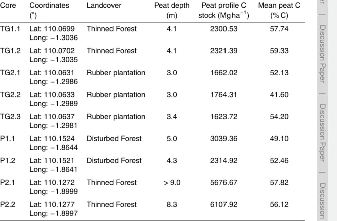
and/or excessive GPR attenuation associated with high electrical conductivity; and (b) variations in the lithology of the sub-peat mineral deposits; and (4) one or more direct soil cores in order to confirm depth of the peat-mineral soil interface and to obtain sam-ples for subsequent C analysis at selected locations. Since not every core collected was analyzed for C content, Table 2 presents a summary of cores collected including

20

average C percent and content along the peat column. Specific results per site are explained below.

4.1 Tanjung Gunung: shallow peat (0–4 m)

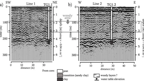
A set of two orthogonal common-oﬀset profiles were collected at Site TG1 with the 0 m distance in Line 1 (Fig. 2a) crossing Line 2 (Fig. 2b) at 24 m along the profile. An

(13)

BGD

12, 191–229, 2015

X. Comas et al.

Title Page

Tables Figures

◭ ◮

Back Close

Full Screen / Esc

Discussion

P

a

per

|

Discussion

P

a

per

|

Discussion

P

a

per

|

Discussion

P

a

per

|

average EM wave velocity of 0.04 m ns−1for the peat column was estimated from GPR common mid-point profiles (not shown here for brevity). Using this velocity estimate, GPR common oﬀset profiles (Fig. 2) identified a 4 m thick peat column that is laterally continuous over the profile.

Direct coring at two locations (shown in Fig. 2a and b respectively) confirms a total

5

peat thickness of 4 m with a 0.1–0.2 m sandy clay transition (also containing some or-ganics) into a clayey mineral soil at about 4.2 m depth. Direct coring also detected the presence of: (1) a water table at 0.5 m depth coinciding with the presence of a distinc-tive reflector in the GPR record (particularly clear in Fig. 2b), (2) a woody area between 2–3 m depth (indicated in Fig. 2) resulting in isolated points of core refusal that

coin-10

cide with the presence of hyperbolic diﬀractions in the reflection record. Extracted core samples showed average of 58.5 % C and C content of 2311.0 Mg ha−1_{(Table 2).}

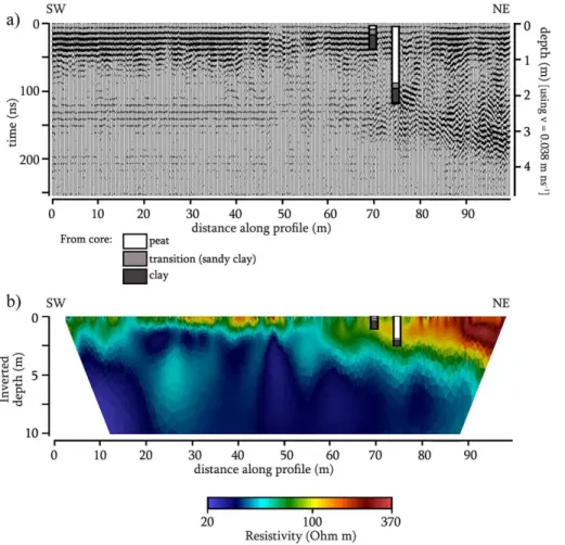
Electrical resistivity imaging results for Line 1 and Line 2 at Site TG1 are shown in Fig. 3a and b respectively. Direct cores as shown in Fig. 2 are superimposed for comparison. The resistivity inversion shows a relatively conductive (resistivity less than

15

100Ωm) upper layer, underlain by a more resistive unit of undetermined thickness. The upper layer (showing a progressive increase in resistivity with depth between 60– 200Ωm) correlates with the terrestrial peat deposit as confirmed from direct sampling and GPR. Resistivity values for the upper layer are comparable with values obtained in northern peatlands and partly attributed to the low ionic concentration of the peat pore

20

water (Slater and Reeve, 2002; Comas et al., 2011b). The underlying resistive layer (ranging between 200–300Ωm) includes both a transition layer composed of a mixture of sand and clay (with some organics) and a clayey mineral soil as confirmed from cor-ing. Although lower resistivities are typical for clayey mineral sediments that are usually found below peat, in this case the higher resistivities are attributed to a sandy mineral

25

(14)

BGD

12, 191–229, 2015

X. Comas et al.

Title Page

Tables Figures

◭ ◮

Back Close

Full Screen / Esc

Discussion

P

a

per

|

Discussion

P

a

per

|

Discussion

P

a

per

|

Discussion

P

a

per

|

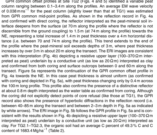
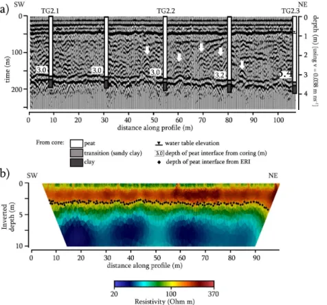
GPR common oﬀset profiles at Site TG2 (Figs. 4 and 5) identified a variable peat column ranging between 0.1–3.4 m along the profiles. An average EM wave velocity of 0.038 m ns−1 for the peat column (slightly lower than that at TG1) was estimated from GPR common mid-point profiles. As shown in the reflection record in Fig. 4a and confirmed with direct coring, the reflector interpreted as the peat-mineral soil

in-5

terface deepens from the surface (at 70 m along the profile where the reflector is not discernible from the ground coupling) to 1.5 m (at 74 m along the profile) towards the NE, representing a total increase of 1.4 m in peat thickness over a 4 m horizontal dis-tance (i.e. between 70 and 74 m along the profile). This trend extends to the end of the profile where the peat-mineral soil exceeds depths of 3 m, where peat thickness

10

increases by over 3 m in about 20 m along the transect. The ERI images are consistent with this interpretation (Fig. 4b) depicting a resistive upper layer (100–370Ωm inter-preted as peat) underlain by a conductive unit (as low as 20Ωm) interpreted as clay and confirmed from both coring and surface outcrops between 0 and 60 m along the transect. Figure 5a represents the continuation of the GPR common oﬀset profile in

15

Fig. 4a towards the NE. In this case peat thickness is almost uniform (as confirmed with coring and depicted in Fig. 5a), with peat thickness changing only by 0.4 m across the 100 m long profile. This profile also confirms the presence of a distinctive reflector at about 0.8 m depth interpreted as the water table as confirmed from coring. Although the coring did not explicitly detect points of core refusal (like those at TG1), the GPR

20

record also shows the presence of hyperbolic diﬀractions in the reflection record (i.e. between 40–85 m along the transect and between 2–3 m depth in Fig. 5a as indicated by white arrows). The ERI image in Fig. 5b follows the GPR profile in Fig. 5a and is con-sistent with the results shown in Fig. 4b depicting a resistive upper layer (100–370Ωm interpreted as peat) underlain by a conductive unit (as low as 20Ωm) interpreted as

25

(15)

BGD

12, 191–229, 2015

X. Comas et al.

Title Page

Tables Figures

◭ ◮

Back Close

Full Screen / Esc

Discussion

P

a

per

|

Discussion

P

a

per

|

Discussion

P

a

per

|

Discussion

P

a

per

|

4.2 Pelang Forest: intermediate and deep peat (5–9 m)

Geophysical surveys constrained with direct coring at Pelang Forest contrast with those previously described at Tanjung Gunung by showing greater peat thicknesses ranging between 5 m at Site P1 up to 9 m at Site P2. GPR and electrical resistivity surveys at Site P1 were collected at diﬀerent locations separated by about 1 km since GPR

tran-5

sects at this site were not accessible with heavy resistivity instrumentation. Similar to Site TG1, an average EM wave velocity of 0.04 m ns−1 _{for the peat column was}

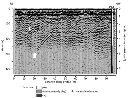
esti-mated from GPR common mid-point profiles at this site. GPR common oﬀset profiles at Site P1 (Fig. 6) show a reflection record characterized by: (1) a depth of penetration of 5 m followed by signal attenuation that coincides with a sandy clay transition (with

10

some organics) between 5–7.5 m underlain by a clayey mineral soil as confirmed from coring (shown at 95 m along the profile in Fig. 6), (2) a distinct reflector at about 35– 40 ns interpreted as the water table, (3) a sequence of laterally discontinuous chaotic reflectors with some hyperbolic diﬀractions (i.e. as seen at 150 ns and 15 m along the profile and indicated by a small white arrow); and (4) a possible depression feature

15

within the peat column between 150–250 ns and 10–35 m along the profile, with a SE side tilting about 9◦ towards the NW and a NW side tilting about 13◦ towards the SE. The white arrow in Fig. 6 indicates the lowest point of this feature. It is important to consider that although migration has not been included in any GPR common oﬀset in order to preserve the appearance of diﬀractions, application of a 1-D Stolt migration in

20

the common oﬀset in Fig. 6 (based on a velocity of 0.04 m ns−1) resulted in changes in the tilt of the reflectors of less than one degree.

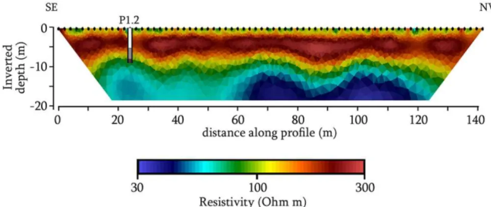
Electrical resistivity imaging results at Site P1 (Fig. 7) show an interface at about 5 m depth (as confirmed from coring) between an upper resistive layer with a resistivity ranging between 150–300Ωm interpreted as peat, underlain by a conductive unit (as

25

(16)

BGD

12, 191–229, 2015

X. Comas et al.

Title Page

Tables Figures

◭ ◮

Back Close

Full Screen / Esc

Discussion

P

a

per

|

Discussion

P

a

per

|

Discussion

P

a

per

|

Discussion

P

a

per

|

units shows intermediate resistivity values (around 100Ωm) and is coincident with the mixture of sand, clay and organics with a thickness of about 2.5 m identified in the cor-ing. Although not directly confirmed from coring, it appears the interface between the peat and the sandy clay is variable across the profile in Fig. 7, indicating an undulat-ing peat thicknesses between 5 m (i.e. at core location at 22 m along the line, and at

5

70, 105, or 120 m along the line based on ERI alone) and 7.5–8 m (i.e. at 12, 90, or 130 m along the profile). The ERI profile also shows a strong lateral resistivity varia-tion in the resistivity of the deeper mineral soil (i.e. below 10 m depth) varying between 30–100Ωm from the SE to the NW direction. Cores P1.1 and P1.2 averaged 50.8 % C with a C content of 2677.1 Mg ha−1(Table 2).

10

Variability in peat thickness at Site P2 (Fig. 8) is similar to that described for Site P1 (Fig. 7) and is confirmed at three coring locations (at 10, 50 and 100 m along the profile) resulting in total peat thicknesses of 9 m or more, 8.7 and 8.8 m respectively. Since topography can be considered flat at the scale of measurement used in this profile, these results confirm that the interface between the peat and the underlying

15

sandy clay transition is undulating and that resistivity values for the peat (between 100–185Ωm) and transitional layer (below 100Ωm) are consistent with those shown in Fig. 7. The clay layer imaged with the resistivity profile in Fig. 7 (and confirmed from coring in that figure) is also visible in Fig. 8 just below the transitional layer and at approximate depths between 10–14 m. Although GPR profiling at this site was also

20

performed using 100 MHz antennas, results are inconclusive (and thus not presented here) since subsurface reflections appear to only penetrate about 3–4 m depth. Site P2 was surveyed during the last day of the field campaign when 50 MHz antennas malfunctioned as explained in the methods section. For cores P2.1 and P2.2 the soils averaged 57.0 % C with a C content of 5892.3 Mg ha−1(Table 2).

(17)

BGD

12, 191–229, 2015

X. Comas et al.

Title Page

Tables Figures

◭ ◮

Back Close

Full Screen / Esc

Discussion

P

a

per

|

Discussion

P

a

per

|

Discussion

P

a

per

|

Discussion

P

a

per

|

5 Discussion

Estimated peat thicknesses are generally consistent between the measurement meth-ods, although several diﬀerences need to be considered. GPR is particularly useful for characterizing peat thickness for shallow peat columns (i.e. TG1 and TG2 in Figs. 2 and 5b respectively) and is able to quantify depth of the peat-mineral soil interface at

5

cm resolution both vertically and laterally from a strong reflector that matches closely with coring results. This reflector resembles the peat-mineral soil interface as typically detected with GPR in boreal peatlands in North America and Europe, exemplified in several studies for those higher latitude systems (Warner et al., 1990; Jol and Smith, 1995; Slater and Reeve, 2002; Parsekian et al., 2012; Comas et al., 2013). However,

10

the GPR method, as based on the antenna frequencies used for this study, shows lim-itations for imaging deep (i.e. 9 m or more) peat columns (i.e. Sites P1 and P2). We attribute these limitations to: (1) thicker peat columns that excessively attenuate the GPR signal, and/or (2) attenuation due to the presence of clay-rich transition layers with high electrical conductivities as depicted by the low resistivity values in P1 and P2

15

(Figs. 7 and 8). Attenuation in clay-rich areas was to be expected since it is well known than the eﬀectiveness of GPR in peatlands is compromised when electrical conductiv-ity of peat is high due to high electrical fluid conduction or high percent of clay (Theimer et al., 1994). Electrical resistivity imaging also proves useful for detecting changes in the peat thickness column across the diﬀerent sites and for estimating the interface

20

between peat and mineral soil. When compared to GPR, electrical resistivity shows similar imaging capabilities for estimating both shallow and deep peat columns in the study areas (due to larger depths of investigation), however resolution (both vertical and lateral) is more limited, particularly as depth increases. The boundaries between the resistive top layer corresponding to the peat and the underlying conductive

ma-25

(18)

BGD

12, 191–229, 2015

X. Comas et al.

Title Page

Tables Figures

◭ ◮

Back Close

Full Screen / Esc

Discussion

P

a

per

|

Discussion

P

a

per

|

Discussion

P

a

per

|

Discussion

P

a

per

|

conductivity is not an accurate indicator of peat thickness when peat is underlain by a conductive layer due to the increase in specific conductance of peat pore fluid to-wards the base of peat and the eﬀect of the mineral soil (Slater and Reeve, 2002). The results presented here also confirm the same issue when peat is underlain by a resis-tive material (Fig. 3). Despite these limitations, a good correspondence exists between

5

the limit of the uppermost high resistivity values at sites TG2, P1 and P2 (depicted in red and orange in Figs. 4b, 7, and 8) and the peat layer interface.

Since the ultimate aim of this work is to increase the accuracy of peat C storage estimates, we consider how geophysical methods may compare to traditional coring methods for estimating carbon stocks. Although the GPR datasets presented in this

10

work are limited particularly in terms of areal extent and scale of measurement, our intent here is to exemplify the potential of the method for enhancing our ability to mea-sure peat thickness and better develop C stock estimates. The profile from Site TG-2 in Fig. 5 can be used to investigate how subtle changes in peat thickness (representing a maximum gradient below 0.02 deg) may influence overall peat and carbon stock

esti-15

mates. Figure 9 shows a comparison between (a) peat thickness estimated from GPR at a total of 539 locations (or every 0.2 m along the profile in Fig. 5a), and direct coring at 5 locations (or approximately every 20 m along the profile) (Fig. 9a); and (b) peat thickness estimated from ERI at a total of 190 locations (interface shown in Fig. 5b), and direct coring at 5 locations (Fig. 9b). Although the regularization constraint used

20

in the ERI inversion procedure has the eﬀect of smoothing structural boundaries, the depth to such boundaries can be estimated in a semi-quantitative way when some kind of ancillary information is available to calibrate the definition of these interfaces. Thus, the lower peat boundary was “picked” from the ERI image using the average inverted resistivity value at pixels corresponding to the interface identified from coring

25

(19)

BGD

12, 191–229, 2015

X. Comas et al.

Title Page

Tables Figures

◭ ◮

Back Close

Full Screen / Esc

Discussion

P

a

per

|

Discussion

P

a

per

|

Discussion

P

a

per

|

Discussion

P

a

per

|

resistivity value. ERI estimates do not consider the first and last 5 m along the profile due to the low resolution in the inversion. GPR estimates in Fig. 9a are based on an average velocity of 0.038 m ns−1 (or a constant relative dielectric permittivity) for the entire peat column. Although EM wave velocity in peat soils most typically range be-tween 0.036–0.044 m ns−1(Parsekian et al., 2012) our average was determined from:

5

(1) the reflector corresponding to the peat-mineral soil interface in GPR common mid-point surveys (consistently showing values of 0.038 m ns−1at two diﬀerent locations at TG2 and using two diﬀerent antenna frequencies); and (2) the travel time recorded at the 5 coring locations (consistently showing estimates 0.038±0.001 m ns−1), thus

rep-resenting a true velocity average of the peat column. Lateral variability in depth to the

10

mineral soil ranges between 2.5–3.5 m along the same transect at TG2 as estimated from the ERI images (Figs. 5b and 9b), confirming (despite the more limited vertical resolution when compared to GPR, as expected) that substrate topography is highly variable laterally. These results also confirm previous studies showing lateral variability in mineral substrate topography across several peat domes in Borneo (Dommain et al.,

15

2010 after Konsultant, 1998).

Error bars in the GPR data (±0.05 m average in Fig. 9a) were calculated from the

diﬀerence in peat thickness between GPR using this average velocity and that mea-sured from the coring. Error bars in the ERI data (Fig. 9b) were computed as the max-imum misfit at each horizontal location between (1) the interpolated interface depth

20

taken from coring and (2) the ERI estimated interface depth using the mean resistiv-ity value±2 SDs. Assuming that lateral variability in peat thickness between cores is

non-existent when the same thickness is estimated for contiguous cores (i.e. perfectly horizontal interface), and that thickness increases gradually with distance (i.e. constant gradient) as shown in the shaded areas in Fig. 9a, the overall peat surface area for

25

(20)

BGD

12, 191–229, 2015

X. Comas et al.

Title Page

Tables Figures

◭ ◮

Back Close

Full Screen / Esc

Discussion

P

a

per

|

Discussion

P

a

per

|

Discussion

P

a

per

|

Discussion

P

a

per

|

peat column in Core TG2.1–TG2.3 (Table 2). Due to the limitations in terms of (a) verti-cal resolution, and (b) lateral extent of the profile (i.e. low inversion results on the edges of the profiles) a similar approach using ERI peat thickness estimates is more uncer-tain and therefore is not included here. Variability in peat thickness was only 2.9–3.4 m (estimated from GPR traces) or 0.4–0.5 m over the 100 m TG2 transect. Although the

5

7 m2 difference in surface area between GPR and coring measurements represents only 0.07 m in average peat thickness, when scaled volumetrically the difference be-tween GPR and coring estimates is 37 Mg C ha−1, which illustrates how relatively small differences in depth estimates can impact overall C storage calculations. Since most peat formations in Indonesia occur at much larger spatial scales (i.e. tens of kilometers

10

or more), GPR surveys over broader areas are shown here to be capable of largely reducing uncertainties regarding peat thickness and C storage. Moreover, as peat C density in tropical peat soils becomes better constrained (Rodríguez et al., 2013), local to regional estimates of peat C storage could be improved through the use of GPR methods to accurately determine peat thickness. Considering peat thickness can also

15

change more dramatically over short distances depending on geomorphic setting (e.g. about 1.5 m diﬀerence in peat thickness within only 4 m along the Site TG-2 profile in Fig. 4), measuring peat thickness at finer spatial resolution would thus significantly improve current C stock estimates. For example other authors have also estimated uncertainties in C storage between 13–25 % due to unconformities of the underlying

20

mineral soil in several peat domes in Central Kalimantan (Jaenicke et al., 2008). More accurate estimates of peat thickness are clearly required to properly define C stocks in Indonesia and likely other tropical peatlands.

The results presented in this work also show potential for improving understand-ing of processes associated with peatland formation as reflected in the diﬀerences in

25

(21)

BGD

12, 191–229, 2015

X. Comas et al.

Title Page

Tables Figures

◭ ◮

Back Close

Full Screen / Esc

Discussion

P

a

per

|

Discussion

P

a

per

|

Discussion

P

a

per

|

Discussion

P

a

per

|

Second, the interface between peat-mineral soil at TG1 and TG2 is characterized by a set of 2–3 sharp reflectors in the GPR record (i.e. Figs. 2, 4, and 5), that is absent at Site P where reflectors are sharply attenuated when reaching depths corresponding to the transition zone between peat and clay. Third, resistivity results do not show marked diﬀerences in terms of electrical conductivity between sites along the peat–clay

inter-5

face, although coring results show a marked increase in thickness of the transition zone (mostly corresponding to mixtures of clay and sand) with averages between 0.1–0.2 m for Sites TG1 and TG2 and averages reaching 2.5 m for Site P1. These diﬀerences may be attributed to two related issues: (1) the developmental history of peatland initiation and formation at each specific site; and (2) the diﬀerences in site location as related to

10

physiographic type of terrain and the characteristics of peat ecosystems at each site. As shown in Fig. 1, sites TG1 and TG2 correspond to MDW or shallow peat swamp ecosystems while sites P1 and P2 are characterized by GBT or large ombrotrophic peat swamp ecosystems. Coastal peat swamps in Kalimantan have been described as the result of peat accumulation developed on marine clay and mangrove deposits of

15

river deltas and coastal plains during the mid Holocene (∼7000–5000 cal BP)

(Ander-son and Muller, 1975; Supiandi, 1988). As sea levels fell around 5000 cal BP, sandy beach ridges were exposed and directly colonized by peat swamps and mud flats were covered by mangroves (Cameron et al., 1989; Dommain et al., 2011). While sites at TG may be related to peat swamp colonization over sandy ridges (as reflected by the

20

presence of a highly resistive mineral soil at TG1 and/or a thin transitional layer at both TG1 and TG2), sites at P may be characterized by colonization of mud flats and mangrove deposits (as characterized by much thicker organomineral mixing horizons and potential increased electrical conductivity that results in a marked attenuation in the GPR reflection record, i.e. Fig. 6). Furthermore, the ERI profiles also show lateral

25

(22)

BGD

12, 191–229, 2015

X. Comas et al.

Title Page

Tables Figures

◭ ◮

Back Close

Full Screen / Esc

Discussion

P

a

per

|

Discussion

P

a

per

|

Discussion

P

a

per

|

Discussion

P

a

per

|

that peat soil undulates at a fine scale. Similar features can also found in Fig. 8 (i.e. between 20–50 m distance along the profile).

Differences in geophysical signatures may also be supported by the difference in C content shown for each specific site. C content for each site is very consistent between cores (Table 2). However, sharp differences exist when comparing sites, showing

val-5

ues (in terms of Mg C ha−1) at P2 that are twofold the averages in P1 or TG1 and three-fold the averages in TG2. Such increases correspond to peat thickness depicting higher C contents for thicker peat columns (e.g. Site P2) and lower C contents for thinner peat columns (e.g. Site TG2). This also appears to be related to type of peat ecosystem as depicted in Table 1, which suggest higher C contents in deep (rather than shallow) peat

10

swamps. The relation between C content variability and peatland type is also supported by previous studies in the region. For example, Shimada et al. (2001) concluded that peatland type was the most important factor controlling volumetric C density in peat-lands of Central Kalimantan mainly due to variability in physical consolidation (mainly porosity) from peat decomposition or nutrient inputs. They also suggested that the

15

those peat soils showing less frequent woody layers (typically corresponding to terrace peat) are more decomposed (i.e. lower porosity) and therefore show higher volumetric C density. Our geophysical results seem to confirm this hypothesis by showing a larger presence of interpreted woody layers in the GPR record along those soils with lower C content values (i.e. TG sites), while P sites (with higher C contents) do not seem

20

to identify a clear presence of wood layers in the GPR record. Site level disturbance and land use history may also contribute substantially to C content of the surface peat, as peat burning, profile mixing, and sedimentation from tailings of canal construction could aﬀect C content.

The spatial resolution provided by GPR common oﬀset profiles shows the potential

25

(23)

BGD

12, 191–229, 2015

X. Comas et al.

Title Page

Tables Figures

◭ ◮

Back Close

Full Screen / Esc

Discussion

P

a

per

|

Discussion

P

a

per

|

Discussion

P

a

per

|

Discussion

P

a

per

|

profile and at 2.5–3 m depth, or in Fig. 5 between 70–85 m distance along the profile and between 2–3 m depth (white arrows in Fig. 5). Diffractions are associated with the presence of objects that may act as isolated reflector points such as cobbles and boul-ders (Neal, 2004). In this case, we associate hyperbolic diffractions in GPR common offsets to the presence of buried woody debris (as further confirmed through coring).

5

Other investigations in northern peatlands have also related GPR diﬀractions to the presence of wood (Slater and Reeve, 2002). Such features are absent at P1 (Fig. 6) where more laterally continuous reflections (i.e. at 3, 4, and 4.5 m depth between 40 to 90 m along the profile) are present. Previous studies in Kalimantan region have also consistently shown layers with large quantities of undecomposed woody fragments

10

heterogeneously distributed within the peat column (Shimada et al., 2001). Further-more, some of these laterally continuous reflectors generate a depressional feature between 10 to 30 m along the profile of P1 (center point indicated by a white arrow in Fig. 6) as depicted by a sharp reflector at depths between 3.5 to almost 6 m that tilts 13 and 9◦ respectively on the NW and SE sides of the profile. Although not directly

con-15

firmed in the field through direct coring, this feature might be related to the presence of buttressed trees which often prompt the formation of hummocks and water ponding upslope (Dommain et al., 2010), or the uprooting of such trees due to wind and the formation of depressional features as the root zone is displaced. Because horizontal reflectors seem to overlap the tilting reflectors may support the hypothesis that the

20

depression formed suddenly, to be later filled up progressively with more peat.

6 Conclusions

This study has demonstrated the potential of GPR and ER imaging for non-invasively mapping the subsurface of peatlands in Indonesia at a spatial resolution previously unreported in tropical peatland systems traditionally measured using coring methods.

25

(24)

BGD

12, 191–229, 2015

X. Comas et al.

Title Page

Tables Figures

◭ ◮

Back Close

Full Screen / Esc

Discussion

P

a

per

|

Discussion

P

a

per

|

Discussion

P

a

per

|

Discussion

P

a

per

|

the peat matrix such as presence of wood layers or buttressed trees, or soil nature as related to peatland ecosystem type (i.e. mangrove vs. freshwater peat). A comparison between peat thickness estimates from GPR, ERI and coring showed a variability ex-ceeding 2 % in peat surface area (or 1191 kg of C assuming C contents of 170 kg C m−2 as averaged from core samples), although this was based on a short 100 m profile

5

showing changes in thickness of less than 0.5 m. Such discrepancies may be larger when considering transects with a more variable peat thickness (such as those here showing up to 1.5 m vertical diﬀerence over only 4 m in the horizontal). Given the dif-ficulty of capturing such variability with traditional methods (such as coring), current C stocks in Indonesian peatlands should be revisited using methods such as GPR or

10

electrical resistivity imaging that better account for lateral variability.

Acknowledgements. This work was supported by the US Agency for International Development (USAID). We are indebted to Kent Elliot (US Forest Service) for all his help with logistics and fieldwork during this study. We are also thankful to Sofyan Kurnianto (CIFOR/Oregon State University) and Ophelia Wang (USAID-IFACS) for their help in the field, and to all the local 15

Indonesians and helpers involved in this research for their support at the study sites. We thank R. Dommain for helpful discussions in some of the materials presented in this study.

References

Ahmed, S. and Carpenter, P. J.: Geophysical response of filled sinkholes, soil pipes and as-sociated bedrock fractures in thinly mantled karst, east-central Illinois, Environ. Geol., 44, 20

705–716, 2003.

Anderson, J. A. R. and Muller, J.: Palynological study of a holocene peat and a miocene coal deposit from NW Borneo, Rev. Palaeobot. Palyno., 19, 291–351, 1975.

Binley, A. and Kemna, A.: DC resistivity and induced polarization methods, in: Hydrogeo-physics, edited by: Rubin, Y. and Hubbard, S. S., Springer, New York, 129–156, 2005. 25

(25)

BGD

12, 191–229, 2015

X. Comas et al.

Title Page

Tables Figures

◭ ◮

Back Close

Full Screen / Esc

Discussion

P

a

per

|

Discussion

P

a

per

|

Discussion

P

a

per

|

Discussion

P

a

per

|

Č_{erven´y, V. and Soares, J.: Fresnel volume ray tracing, Geophysics, 57, 902–915, 1992.} Comas, X. and Slater, L.: Low-frequency electrical properties of peat, Water Resour. Res., 40,

W12414, doi:10.1029/2004WR003534, 2004.

Comas, X. and Slater, L.: Evolution of biogenic gasses in peat blocks inferred from non-invasive dielectric permittivity measurements, Water Resour. Res., 43, W05424, 5

doi:10.1029/2006WR005562, 2007.

Comas, X., Slater, L., and Reeve, A.: Geophysical evidence for peat basin morphology and stratigraphic controls on vegetation observed in a Northern Peatland, J. Hydrol., 295, 173– 184, 2004.

Comas, X., Slater, L., and Reeve, A.: Spatial variability in biogenic gas accumulations in peat 10

soils is revealed by ground penetrating radar (GPR), Geophys. Res. Lett., 32, L08401, doi:10.1029/2004GL022297, 2005a.

Comas, X., Slater, L., and Reeve, A.: Stratigraphic controls on pool formation in a domed bog inferred from ground penetrating radar (GPR), J. Hydrol., 315, 40–51, 2005b.

Comas, X., Slater, L., and Reeve, A.: In situ monitoring of ebullition from a peat-15

land using ground penetrating radar (GPR), Geophys. Res. Lett., 34, L06402, doi:10.1029/2006GL029014, 2007.

Comas, X., Slater, L., and Reeve, A.: Seasonal geophysical monitoring of biogenic gases in a northern peatland: implications for temporal and spatial variability in free phase gas pro-duction rates, J. Geophys. Res., 113, G01012, doi:10.1029/2007JG000575, 2008.

20

Comas, X., Slater, L., and Reeve, A.: Atmospheric pressure drives changes in the vertical distribution of biogenic free-phase gasses in a northern peatland, J. Geophys. Res.-Biogeo., 116, G04014, doi:10.1029/2011JG001701, 2011a.

Comas, X., Slater, L., and Reeve, A. S.: Pool patterning in a northern peatland: geophysical evidence for the role of postglacial landforms, J. Hydrol., 399, 173–184, 2011b.

25

Comas, X., Kettridge, N., Binley, A., Slater, L., Parsekian, A., Baird, A. J., Strack, M., and Waddington, J. M.: The eﬀect of peat structure on the spatial distribution of biogenic gases within bogs, Hydrol. Process., 28, 5483–5494, doi:10.1002/hyp.10056, 2013.

Coscia, I., Greenhalgh, S. A., Linde, N., Doetsch, J., Marescot, L., Günther, T., Vogt, T., and Green, A. G.: Three-dimensional geophysical mapping: providing new constraints for under-30

(26)

BGD

12, 191–229, 2015

X. Comas et al.

Title Page

Tables Figures

◭ ◮

Back Close

Full Screen / Esc

Discussion

P

a

per

|

Discussion

P

a

per

|

Discussion

P

a

per

|

Discussion

P

a

per

|

Dommain, R., Couwenberg, J., and Joosten, H.: Hydrological self-regulation of domed peat-lands in south-east Asia and consequences for conservation and restoration, Mires and Peat, 6, 1–17, 2010.

Dommain, R., Couwenberg, J., and Joosten, H.: Development and carbon sequestration of tropical peat domes in south-east Asia: links to post-glacial sea-level changes and Holocene 5

climate variability, Quaternary Sci. Rev., 30, 999–1010, 2011.

Geuzaine, C. and Remacle, J. F.: Gmsh: a three-dimensional finite element mesh generator with built-in pre- and post-processing facilities, Int. J. Numer. Meth. Eng., 79, 1309–1331, 2009.

Holden, J., Burt, T. P., and Vilas, M.: Application of ground-penetrating radar to the identification 10

of subsurface piping in blanket peat, Earth Surf. Proc. Land., 27, 235–249, 2002.

Hooijer, A., Silvius, M., W osten, H., and Page, S.: PEAT-CO2, Assessment of CO₂emissions from drained peatlands in SE Asia, Delft Hydraulics report Q3943/2006, p. 36, available at: http://peat-co2.deltares.nl, 2006

Jaenicke, J., Rieley, J. O., Mott, C., Kimman, P., and Siegert, F.: Determination of the amount of 15

carbon stored in Indonesian peatlands, Geoderma, 147, 151–158, 2008.

Jol, H. M. and Smith, D. G.: Ground penetrating radar surveys of peatlands for oilfield pipelines in Canada, J. Appl. Geophys., 34, 109–123, 1995.

Joosten, H.: The Global Peatland CO₂Picture, Ede, Wetlands International, 2009.

Kettridge, N., Comas, X., Baird, A., Slater, L., Strack, M., Thompson, D., and Jol, H.: 20

Ecohydrologically-important subsurface structures in peatlands are revealed by Ground-Penetrating Radar and resistivity measurements, J. Geophys. Res.-Biogeo., 113, G04030, doi:10.1029/2008JG000787, 2008.

Kettridge, N., Binley, A., Comas, X., Cassidy, N., Baird, A., Harris, A., van der Kruk, J., Strack, M., Milner, A., and Waddington, J. M.: Do peatland microforms move through time? 25

Examining the developmental history of a patterned peatland using ground penetrating radar, J. Geophys. Res.-Biogeo., 117, G03030, doi:10.1029/2011JG001876, 2012.

Konsultant, P. S.: Detailed Design and Construction Supervision of Flood Protection and Drainage Facilities for Balingian RGC Agricultural Development Project, Sibu Division, Sarawak (Inception Report), Kuching, 1998.

30

(27)

BGD

12, 191–229, 2015

X. Comas et al.

Title Page

Tables Figures

◭ ◮

Back Close

Full Screen / Esc

Discussion

P

a

per

|

Discussion

P

a

per

|

Discussion

P

a

per

|

Discussion

P

a

per

|

Lowry, T., Allen, M. B., and Shive, P. N.: Singularity removal: a refinement of resistivity modeling techniques, Geophysics, 54, 766–774, 1989.

Menke, W.: Geophysical Data Analysis: Discrete Inverse Theory, Academic Press Inc., New York, 1989.

Meyer, J. H.: Investigation of Holocene organic sediments: a geophysical approach, Int. Peat 5

J., 3, 45–57, 1989.

Neal, A.: Ground-penetrating radar and its use in sedimentology: principles, problems and progress, Earth-Sci. Rev., 66, 261–330, 2004.

Page, S. E., Rieley, J. O., and Banks, C. J.: Global and regional importance of the tropical peatland carbon pool, Glob. Change Biol., 17, 798–818, 2011.

10

Parsekian, A., Slater, L., Comas, X., and Glaser, P.: Variations in free-phase gases in peat land-forms determined by ground – penetrating radar, J. Geophys. Res.-Biogeosci., 115, G02002, doi:10.1029/2009JG001086, 2010.

Parsekian, A., Comas, X., Slater, L., and Glaser, P. H.: Geophysical evidence for the lateral distribution of free phase gas at the peat basin scale in a large northern peatland, J. Geophys. 15

Res., 116, G03008, doi:10.1029/2010JG001543, 2011.

Parsekian, A. D., Slater, L., Sebestyen, S. D., Kolka, R. K., Ntarlagiannis, D., Nolan, J., and Hanson, P.: Comparison of uncertainty in peat volume and soil carbon estimated using GPR and probing, Soil Sci. Soc. Am. J., 76, 1911–1918, 2012.

RePPProT, Regional Physical Planning Programme for Transmigration: The Land Resources 20

of Indonesia: a National Overview, Main Report, Ministry of Transmigration and Land Re-sources Department/Bina Program, Jakarta, 1990.

Robinson, J., Johnson, T., and Slater, L. D.: Evaluation of regularization constraints for improv-ing electrical resistivity imagimprov-ing of discrete fractures, Geophysics, 78, D115–D127, 2013. Rodríguez, V., Gutiérrez, F., Green, A. G., Carbonel, D., Horstmeyer, H., and Schmelzbach, C.: 25

Characterising saging and collapse sinkholes in a mantled karst by means of Ground Pene-trating Radar (GPR), Environ. Eng. Geosci., 20, 109–132, doi:10.2113/gseegeosci.20.2.109, 2014.

Shimada, S., Takahashi, H., Haraguchi, A., and Kaneko, M.: The carbon content characteris-tics of tropical peats in Central Kalimantan, Indonesia: estimating their spatial variability in 30

(28)

BGD

12, 191–229, 2015

X. Comas et al.

Title Page

Tables Figures

◭ ◮

Back Close

Full Screen / Esc

Discussion

P

a

per

|

Discussion

P

a

per

|

Discussion

P

a

per

|

Discussion

P

a

per

|

Slater, L. and Binley, A.: Synthetic and field-based electrical imaging of a zerovalent iron bar-rier: implications for monitoring long-term barrier performance, Geophysics, 71, B129–B137, 2006.

Slater, L. and Reeve, A.: Understanding peatland hydrology and stratigraphy using integrated electrical geophysics, Geophysics, 67, 365–378, 2002.

5

Slater, L., Binley, A. M., Daily, W., and Johnson, R.: Cross-hole electrical imaging of a controlled saline tracer injection, J. Appl. Geophys., 44, 85–102, 2000.

Slater, L., Comas, X., Ntarlagiannis, D., and Roy Moulik, M.: Resistivity-based monitoring of bio-genic gasses in peat soils, Water Resour. Res., 43, W10430, doi:10.1029/2007WR006090, 2007.

10

Supiandi, S.: Studies on peat in the coastal plains of Sumatra and Borneo. Part I: Physiography and geomorphology of the coastal plains, Southeast Asian Studies, 26, 308–335, 1988. Theimer, B. D., Nobes, D. C., and Warner, B. G.: A study of the geoelectrical properties of

peatlands and their influence on ground-penetrating radar surveying, Geophys. Prospect., 42, 179–209, 1994.

15

van Schoor, M.: Detection of sinkholes using 2D electrical resistivity imaging, J. Appl. Geophys., 50, 393–399, 2002.

Wahyunto, Ritung, S., and Subagjo, H.: Peta Luas Sebaran Lahan Gambut danKandungan Karbon di Pulau Sumatera/Maps of Area of Peatland Distribution and Carbon Content in Sumatera, 1990–2002, Wetlands International – Indonesia Programme and Wildlife Habitat 20

Canada (WHC), Bogor, 2003.

Wahyunto, Ritung, S., and Subagjo, H.: Peta Sebaran Lahan Gambut, Luas dan Kandungan Karbon di Kalimantan/Map of Peatland Distribution Area and Carbon Content in Kalimantan, 2000–2002, Wetlands International – Indonesia Programme and Wildlife Habitat Canada (WHC), Bogor, 2004.

25

Warner, B. G., Nobes, D. C., and Theimer, B. D.: An application of ground penetrating radar to peat stratigraphy of Ellice Swamp, southwestern Ontario, Can. J. Earth Sci., 27, 932–938, 1990.

Worfield, R. D., Parashar, S. K., and Perrot, T.: Depth profiling of peat deposits with impulse radar, Can. Geotech. J., 23, 142–154, 1986.

30