Quasi-3-D resistivity imaging – mapping of heterogeneous frozen ground conditions using electrical resistivity tomography

(1)

TCD

3, 895–918, 2009

Quasi-3-D resistivity imaging

C. Kneisel et al.

Title Page

Abstract Introduction

Conclusions References

Tables Figures

◭ ◮

Back Close

Full Screen / Esc

Printer-friendly Version

Interactive Discussion The Cryosphere Discuss., 3, 895–918, 2009

www.the-cryosphere-discuss.net/3/895/2009/ © Author(s) 2009. This work is distributed under the Creative Commons Attribution 3.0 License.

The Cryosphere Discussions

This discussion paper is/has been under review for the journal The Cryosphere (TC). Please refer to the corresponding final paper in TC if available.

Quasi-3-D resistivity imaging – mapping

of heterogeneous frozen ground

conditions using electrical resistivity

tomography

C. Kneisel, A. Bast, and D. Schwindt

Department of Physical Geography, University of W ¨urzburg, Germany

Received: 18 October 2009 – Accepted: 21 October 2009 – Published: 30 October 2009 Correspondence to: C. Kneisel (kneisel@uni-wuerzburg.de)

(2)

TCD

3, 895–918, 2009

C. Kneisel et al.

Title Page

Tables Figures

◭ ◮

Back Close

Full Screen / Esc

Interactive Discussion

Abstract

Up to now an efficient 3-D geophysical mapping of the subsurface in mountainous environments with rough terrain has not been possible. A merging approach of several closely spaced 2-D electrical resistivity tomography (ERT) surveys to build up a quasi-3-D model of the electrical resistivity is presented herein as a practical compromise 5

for inferring subsurface characteristics and lithology. The ERT measurements were realised in a small glacier forefield in the Swiss Alps with complex terrain exhibiting a small scale spatial variability of surface substrate.

To build up the grid for the quasi-3-D measurements the ERT surveys were arranged as parallel profiles and perpendicular tie lines. The measured 2-D datasets were col-10

lated into one quasi-3-D file. A forward modelling approach – based on studies at a permafrost site below timberline – was used to optimize the geophysical survey de-sign for the mapping of the mountain permafrost distribution in the investigated glacier forefield.

Quasi-3-D geoelectrical imaging is a useful method for mapping of heterogeneous 15

frozen ground conditions and can be considered as a further milestone in the applica-tion of near surface geophysics in mountain permafrost environments.

1 Introduction

Frozen ground is a widespread phenomenon in alpine and subarctic cold environments. Climate change and its impact on the cryosphere is a topic of increasing importance, 20

due to the growing concern of warming induced permafrost degradation and its conse-quences regarding slope instabilities, construction failure and other hazards related to thermal perturbations and the melting of ground ice in alpine environments (e.g. Harris et al., 2009).

The occurrence of mountain permafrost strongly depends on elevation, incoming 25

(3)

TCD

3, 895–918, 2009

C. Kneisel et al.

Title Page

Tables Figures

◭ ◮

Back Close

Full Screen / Esc

Interactive Discussion warming climate, permafrost is likely to disappear first from marginal areas with mean

annual temperatures close to 0◦_{C, while the greatest terrain disturbance will occur in}

areas with the largest amount of near-surface ground ice.

Many important problems in cryospheric sciences, such as warming-induced per-mafrost degradation, concern properties and processes taking place in the shallow 5

subsurface. The often heterogeneous surface and subsurface conditions in periglacial environments call for methods that are able to resolve the shallow subsurface. Geo-physical methods provide information on the Geo-physical properties of the subsurface, the spatial distribution of these properties, and by inference, on the structure of the subsurface. Furthermore, geophysical techniques can be applied rapidly and at low 10

cost. They have been widely used to characterise areas of perennially frozen ground and locate massive ground ice. Their successful application within cold environments is based on changes in physical properties that occur following the phase change from unfrozen to frozen state. Because deep drilling in permafrost is expensive, time-consuming and logistically demanding, the direct examination of the subsurface is sel-15

dom possible in remote locations. This constitutes one of the main reasons for using geophysical methods instead (Kneisel et al., 2008). These non- or minimally-invasive geophysical methods can rapidly provide information over an entire survey area in con-trast to the point-source information available from drill sites. Modern data acquisition techniques allow geophysical mapping of the subsurface conditions even in heteroge-20

neous mountain environments. However, drill sites remain important to improve the interpretation of data from geophysical surveys. A detailed description of different geo-physical methods for permafrost detection is given in Hauck and Kneisel (2008). For a review on recent advances in geophysical methods for permafrost investigations see Kneisel et al. (2008).

25

(4)

TCD

3, 895–918, 2009

C. Kneisel et al.

Title Page

Tables Figures

◭ ◮

Back Close

Full Screen / Esc

Interactive Discussion Hauck, 2008). ERT is a comparatively fast method to image the subsurface and infer

permafrost characteristics even on rugged alpine terrain with rough surface conditions. While 2-D geophysical techniques can be regarded as the standard state-of-the-art technology, (quasi-) 3-D applications are still in their infancy in the study of mountain permafrost.

5

Up to now an efficient 3-D geophysical mapping of the subsurface in mountainous environments with rough terrain has not been possible. As a realistic compromise, re-sults of several 2-D geophysical surveys at close distance can be merged to build up a quasi-3-D image of the subsurface characteristics and lithology. This new applica-tion of quasi-3-D geoelectrical imaging for mapping permafrost condiapplica-tions is presented 10

herein. This approach has been followed at a recently exposed glacier forefield with discontinuous permafrost and also at a site with isolated permafrost lenses below tim-berline (Bast and Kneisel, 2009; Kneisel and Bast, 2009; Schwindt and Kneisel, 2009). Forward modelling of synthetic data was used to improve the application of 2-D ERT with regard to quasi-3-D imaging. Supported by temperature data from a nearby shal-15

low borehole this approach allows a more sophisticated interpretation of the distribution and characteristics of frozen ground in heterogeneous permafrost environments.

2 Sites

Due to often small-scale spatial variability of surface textural characteristics, recently exposed glacier forefields at high altitude are favourable environments to study the 20

heterogeneous alpine permafrost distribution and its characteristics. The investigated glacier forefield Muragl (46◦₃₀′₁₅′′_{N, 9}◦₅₆′₃₀′′_{E) is located in the Upper Engadine,}

eastern Swiss Alps. It extends in elevation from 2650 m to 2900 m a.s.l. and consists of glacial till of different grain sizes (coarse-grained to fine-grained). The bedrock is made of gneiss and mica schists. This glacier forefield was extensively studied using a vari-25

(5)

log-TCD

3, 895–918, 2009

C. Kneisel et al.

Title Page

Tables Figures

◭ ◮

Back Close

Full Screen / Esc

Interactive Discussion ging, photogrammetrical measurements, GIS-based models). The study site was also

investigated using a high number of parallel, overlapping and perpendicular ERT pro-files to cross-check the quality of the measurements and enhance the interpretation of the obtained 2-D results (cf. Kneisel, 2004; Kneisel and K ¨a ¨ab, 2007).

The site with isolated permafrost lenses below the timberline is located in the Bever 5

Valley, a trough-shaped valley with bottom elevation between 1730 m and 1800 m a.s.l. at its lower end. Both the north- and south-exposed valley sides are wooded. First investigations of the permafrost below timberline in the Bever Valley started ten years ago including BTS-measurements and 1-D and 2-D geoelectrical soundings (Kneisel et al., 2000). For a detailed geophysical mapping of the sporadic permafrost distribu-10

tion joint application of electrical resistivity tomography (ERT) and seismic refraction tomography (SRT) have been applied recently (Kneisel and Schwindt, 2008). Based on the site specific knowledge of the geophysical properties, the forward modelling approach was performed (Schwindt and Kneisel, 2009).

3 Methods

15

The 2-D electrical surveys were performed using an IRIS SYSCAL Junior Switch resistivity-meter. Choice of the appropriate electrode configuration was dependent on the difficult surface conditions associated with the periglacial mountain environment. Since the maximum current injected into the ground can be quite low, the geometri-cal factors of the electrode configurations may be critigeometri-cal. For this reason, Wenner 20

and Wenner-Schlumberger configurations have been employed, even though a Dipole-Dipole configuration could provide superior lateral resolution. Because of high con-tact resistances of the rocky ground surface in some parts of the measurement grid, sponges soaked in water were used at some electrodes to establish sufficient electrical contact to the ground.

25

(6)

TCD

3, 895–918, 2009

C. Kneisel et al.

Title Page

Tables Figures

◭ ◮

Back Close

Full Screen / Esc

Interactive Discussion the grid for the quasi-3-D measurements, the ERT surveys were arranged as 10 parallel

profiles and 7 perpendicular tie lines. Measured 2-D datasets were collated into one quasi-3-D file using the software package Res2Dinv (Loke, 2004). Res3Dinv was used to perform a true 3-D smoothness-constrained inversion using finite difference forward modelling and quasi-Newton inversion techniques (Loke and Barker, 1995, 1996). 5

The specific subsurface distribution of electrical resistivity can be assessed from the inversion of the values of observed apparent electrical resistivity. The general aim of the geophysical inversion is to find a subsurface model that best fits the observed data. The term inversion comes from the inverse problem in contrast to the forward problem where a set of geophysical data is predicted from a specific subsurface distribution of 10

geophysical properties (cf. Kneisel et al., 2008 and see further below). The optimisa-tion method tries to reduce the difference between calculated and measured apparent resistivity values by adjusting the resistivity of the model blocks. A measure of this dif-ference is given by the root-mean-square error (RMS). However, the best model from a geomorphological or geological perspective might not be the one with the lowest 15

possible RMS. Thus, it is essential to consider the local geomorphological setting in performing the interpretation. This enables unrealistic images of the subsurface struc-ture to be excluded. Additionally, topography was incorporated in the inversion routine, which is an important factor in mountainous terrain. For interpretation the quasi-3-D model was visualised as depth slices and block diagrams.

20

Within the forward modelling approach a subsurface model is developed using the information available on a given medium. Subsequently, a synthetic geophysical model is derived from the geological model using appropriate or known geophysical proper-ties for each layer constituting the subsurface model. Finally, forward modelling of the synthetic geophysical model leads to a set of predicted geophysical data. These 25

(7)

TCD

3, 895–918, 2009

C. Kneisel et al.

Title Page

Tables Figures

◭ ◮

Back Close

Full Screen / Esc

Interactive Discussion range of physical properties affecting the geophysical property of interest, expected

subsurface distribution of physical properties) (see Fortier et al., 2008 and Kneisel et al., 2008 for more details).

First attempts of quasi-3-D imaging, based on extensive geophysical mapping in the Bever Valley (Kneisel and Schwindt, 2008) indicate that the most important factors 5

influencing data quality are parallel spacing and the information of perpendicular cross-ing profiles (tie lines). A survey line separation of less than double electrode spaccross-ing, as often recommended (Loke, 2004) can hardly be applied e_fficiently in mountainous regions.

A number of synthetic 2-D ERT profiles were generated, using the forward modelling 10

software Res2Dmod (Loke, 2004). Design of the synthetic profiles was geared on the surveys measured in the Bever Valley. The modelled 2-D files were collated into a D file and inverted using the software Res2Dinv/Res3Dinv. Synthetic quasi-3-D images were modelled using di_fferent array types (Wenner, Wenner-Schlumberger and Dipole-Dipole), electrode spacing (2 m and 3 m) and parallel line separation (dou-15

ble, triple and quadruple). To evaluate the influence of tie lines, quasi-3-D images were modelled using only parallel profiles as well as quasi-3-D images containing a combination of parallel profiles and perpendicular tie lines.

4 Results and discussion

In 2008 two permafrost occurrences, one with fine- to medium-grained surface material 20

and one with medium- to coarse-grained material have been investigated using 17 and 22 ERT profiles, respectively, to build up the 3-D images of the subsurface. In the following, the results of the fine- to medium-grained site are presented. The 17 surveys consist of 10 parallel profiles and 7 perpendicular tie lines (cf. Table 1).

To evaluate the influence of the number of longitudinal and horizontal surveys as well 25

(8)

TCD

3, 895–918, 2009

C. Kneisel et al.

Title Page

Tables Figures

◭ ◮

Back Close

Full Screen / Esc

Interactive Discussion resolution, depth of investigation) of different electrode spacing and array types can be

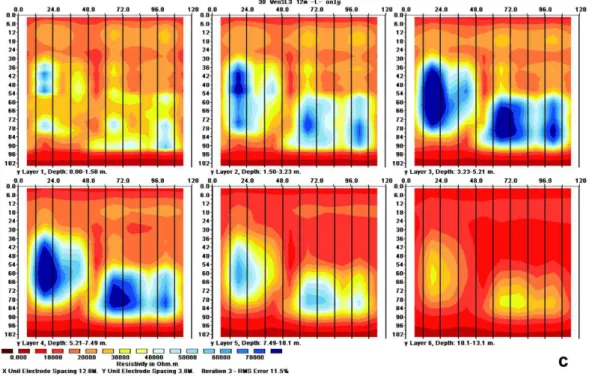
transferred from 2-D ERT is confirmed. Choice of electrode spacing and array type depend on site characteristics and objectives of the project. The application of only parallel arrays results in line-like structures and loss of information value with larger parallel spacings (cf. Fig. 1a, b, c). The influence of measurements in perpendicular 5

directions is shown in Figs. 2 and 3. Both images are based on the same model shown in Fig. 1b (triple electrode spacing and Wenner-Schlumberger array) including perpen-dicular transects. The modelled cross-profiles, that were used to build up the quasi-3-D image of Fig. 2, contain information of a single high-resistive anomaly between horizon-tal distance 48–93 m of the ERT (cf. Fig. 4), while the modelled perpendicular transects 10

included in Fig. 3 show a separation of the anomaly (cf. Fig. 5). The resulting quasi-3-D image shows one single or a divided anomaly, depending on the information of perpendicular tie lines. In both cases the use of measurements in two perpendicu-lar directions helps to reduce the bias in the quasi-3-D datasets resulting from perpendicu-larger parallel spacing.

15

Results from forward modelling indicate that a parallel spacing between transects should not be larger than quadruple electrode spacing, while triple spacing has proven to be a good agreement between resolution and efficiency (Schwindt and Kneisel, 2009). Enlarging the distance between transects results in a loss of information value and a blurred illustration of resistivity anomalies. A high number of perpendicular tie 20

lines is of importance for achieving a reliable quasi-3-D image.

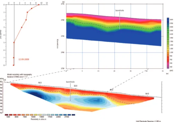
The findings from the forward modelling approach were used to optimize the 3-D survey design within the Muragl glacier forefield. To confirm and characterise the per-mafrost occurrence ERT surveys were used in conjunction with SRT and borehole temperature data (Fig. 6).

25

(9)

TCD

3, 895–918, 2009

C. Kneisel et al.

Title Page

Tables Figures

◭ ◮

Back Close

Full Screen / Esc

Interactive Discussion varies between 4–7 m (indicated by the dashed-line in Fig. 6), an interpretation which

is congruent in both, SRT (<2000 m/s) and ERT survey (<9 kOhm m). Borehole

tem-peratures – measured in September 2008 – denote an active layer thickness of 5 m and a minimum permafrost temperature of−0.25◦C at 8 m depth.

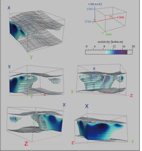
The subsurface heterogeneity with permafrost occurrences and permafrost free ar-5

eas at close distance is visualised in Figs. 7 and 8. Resistivitiy values range from about 1 kOhm m up to a maximum value of 22 kOhm m. Based on borehole temperature mea-surements in combination with results of time-lapse geoelectrical monitoring, the value of 9 kOhm m could be deduced as the lower boundary resistivity value representing permafrost conditions in the area to be mapped. The relatively low resistivity values 10

are interpreted as permafrost occurrences that consist of frozen material with di_fferent grain sizes (pore ice), as a saturated or supersaturated massive ice layer would re-sult in much higher resistivities (Kneisel and K ¨a ¨ab, 2007). Resistivities between 9 and 12 kOhm m and low P-wave velocities between 1500–2000 m/s indicate a high content of unfrozen water in the margins of the permafrost lenses. Resistivity values greater 15

than 12 kOhm m and velocities between 2000 m/s and 3000 m/s suggest higher ice contents in the central parts of the permafrost lenses.

The permafrost distribution at this site depends on topography, surface textural char-acteristics as well as snow cover and duration. The active-layer thickness exceeding 5 m in places and the isolated small permafrost lens, visible in Fig. 8, point to degrad-20

ing permafrost. Previous 2-D ERT surveys confirm this interpretation. Hence, there is active permafrost which seems to be in equilibrium with the local climatic conditions and degrading permafrost in close proximity (Kneisel, 2004; Kneisel and K ¨a ¨ab, 2007).

Measurements in the Bever Valley and in the Muragl glacier forefield as well as syn-thetic forward modelling indicate that reliable data can be achieved using larger line 25

(10)

TCD

3, 895–918, 2009

C. Kneisel et al.

Title Page

Tables Figures

◭ ◮

Back Close

Full Screen / Esc

Interactive Discussion field surveys confirm that good data quality and spatial resolution of the subsurface

model can be achieved by using triple electrode spacing between parallel surveys in combination with perpendicular tie lines (Bast and Kneisel, 2009).

5 Conclusions and perspectives

Quasi 3-D geoelectrical imaging can be considered as a further milestone in the ap-5

plication of near surface geophysics for frozen ground mapping in heterogeneous per-mafrost environments. Key results and recommendations of our studies include:

– geoelectrical mapping has proven to be a promising approach at these complex permafrost sites to assess subsurface heterogeneity in detail;

– good data quality of the single 2-D data sets is a precondition to obtain reason-10

able results for the quasi-3-D model of the subsurface, hence coupling of the electrodes to the sometimes rough terrain with rugged topography has to be done thoroughly;

– forward modelling of synthetic 2-D and quasi-3-D data is a useful tool for designing geophysical surveys to optimise field procedure;

15

– survey line separation should not be larger than quadruple electrode spacing while triple spacing has proven to be a good compromise between efficient data acquisition, resolution and realistic model of the subsurface;

– application of tie lines is important to assure data quality and to reduce bias;

– in case of large resistivity contrast, reliable distinctions can be made between 20

(11)

TCD

3, 895–918, 2009

C. Kneisel et al.

Title Page

Tables Figures

◭ ◮

Back Close

Full Screen / Esc

Interactive Discussion High-altitude alpine permafrost environments often exhibit a distinct small-scale

het-erogeneity of permafrost distribution as well as surface and subsurface characteristics. Questions arise concerning the degree of heterogeneity. Hence, knowledge of the dis-tribution pattern and the factors determining the presence or absence of permafrost under di_fferent environmental conditions, especially at the fringe of discontinuous and 5

sporadic permafrost occurrences, is a key to assess ongoing and future impact of cli-mate change. Up to now an efficient 3-D geophysical mapping of the subsurface in mountainous environments with rough terrain has not been possible. The presented approach of merging several closely spaced 2-D ERT surveys to build up a quasi-3-D image of the subsurface characteristics and lithology is considered as a practical 10

compromise. The quasi-3-D image allows an easier comparison with results of e.g. geomorphological mapping and more sophisticated conclusions can be drawn regard-ing the influence of atmospheric temperature and snow cover evolution on the subsur-face ground temperature regime and hence permafrost degradation, preservation or aggradation. Furthermore, this approach could become increasingly important for the 15

assessment of potential hazards associated with ice-rich mountain permafrost and the small-scale verification of permafrost models.

Acknowledgements. The author C. Kneisel gratefully acknowledges the German Research

Foundation (DFG) for financial support of the Pils-project (permafrost in loose sediments). D. Schwindt gratefully acknowledges the “Bayerische Graduiertenf ¨orderung (BayEFG)”. 20

References

Bast, A. and Kneisel, C.: Quasi-3-D geoelectrical imaging as a new application for permafrost investigations: some methodological aspects, EGU General Assembly, Vienna, Austria, 19– 24 April 2009, EGU2009-5302, 2009.

Fortier, R., LeBlanc, A. M., Allard, M., Buteau, S., and Calmels, F.: Internal structure and condi-25

(12)

TCD

3, 895–918, 2009

C. Kneisel et al.

Title Page Abstract Introduction Conclusions References Tables Figures ◭ ◮ ◭ ◮ Back Close

Full Screen / Esc

Interactive Discussion Harris, C., Arenson, L. U., Christiansen, H. H., Etzelm ¨uller, B., Frauenfelder, R., Gruber, S.,

Haeberli, W., Hauck, C., Hoelzle, M., Humlum, O., Isaksen, K., K ä äb, A., Kern-Luetschg, M. A., Lehning, M., Matsuoka, N., Murton, J. B., Noetzli, J., Phillips, M., Ross, N., Sepp äl ä, M. Springman, S. M., and Vonder M ühll, D.: Permafrost and climate in Europe: Monitoring and modelling thermal, geomorphological and geotechnical responses, Earth Sci. Rev., 92(3–4), 5

117–171, 2009.

Hauck, C. and Kneisel, C. (Eds.): Applied Geophysics in Periglacial Environments, Cambridge University Press, Cambridge, New York, 240 pp., 2008.

Kneisel, C.: New insights into mountain permafrost occurrence and characteristics in glacier forefields at high altitude through the application of 2-D resistivity imaging, Permafrost 10

Periglac., 15, 221–227, 2004.

Kneisel, C.: The nature and dynamics of frozen ground in alpine and subarctic periglacial environments, The Holocene, accepted, 2009.

Kneisel, C. and Hauck, C.: Electrical methods, in: Applied geophysics in periglacial environ-ments, edited by: Hauck, C. and Kneisel, C., Cambridge University Press, Cambridge, New 15

York, 1–27, 2008.

Kneisel, C. and Bast, A.: Looking inside – using a traditional method for permafrost investigation with a new application: 3-D Geoelectrical Imaging, EGU General Assembly, Vienna, Austria, 19–24 April 2009, EGU2009-5067, 2009.

Kneisel, C. and K ¨a ¨ab, A.: Mountain permafrost dynamics within a recently exposed glacier 20

forefield inferred by a combined geomorphological, geophysical and photogrammetrical ap-proach, Earth Surf. Proc. Land., 32(12), 1797–1810, 2007.

Kneisel, C. and Schwindt, D.: Geophysical mapping of isolated permafrost lenses at a spo-radic permafrost site at low altitude in the Swiss Alps, Proceedings of the 9th International Conference on Permafrost, Fairbanks, Alaska, USA, 29 June–3 July, 959–964, 2008. 25

Kneisel, C., Hauck, C., and Vonder M ¨uhll, D.: Permafrost below the timberline confirmed and characterized by geoelectrical resistivity measurements, Bever Valley, eastern Swiss Alps, Permafrost Periglac., 11, 295–304, 2000.

Kneisel, C., Hauck, C., Fortier, R., and Moorman, B.: Advances in geophysical methods for permafrost investigations, Permafrost Periglac., 19(2), 157–178, 2008.

30

Loke, M. H.: Tutorial: 2-D and 3-D electrical imaging surveys, online available at: http://www. geoelectrical.com/coursenotes.zip, 2004.

(13)

pseudosec-TCD

3, 895–918, 2009

C. Kneisel et al.

Title Page

Tables Figures

◭ ◮

Back Close

Full Screen / Esc

Interactive Discussion tions, Geophysics, 60, 1682–1690, 1995.

Loke, M. H. and Barker, R. D.: Practical techniques for 3-D resistivity surveys and data inver-sion, Geophys. Prospect., 44, 499–523, 1996.

Marescot, L., Loke, M. H., Chappellier, D., Delaloye, R., Lambiel, C., and Reynard, E.: As-sessing reliability of 2-D resistivity imaging in mountain permafrost studies using the depth 5

of investigation index method, Near Surf. Geophys., 1, 57–67, 2003.

(14)

TCD

3, 895–918, 2009

C. Kneisel et al.

Title Page

Tables Figures

◭ ◮

Back Close

Full Screen / Esc

Table 1.Details of the ERT surveys and the quasi-3-D ERT image.

Electrode array Wenner-Schlumberger

(inline) electrode spacing 2 m Survey line separation 6 m Tie line separation variable RMS-error after 6 iterations 4.72% Maximum of pseudo depth 28.8 m No. of eliminated data points 32 (of 4896)

(15)

TCD

3, 895–918, 2009

C. Kneisel et al.

Title Page

Tables Figures

◭ ◮

Back Close

Full Screen / Esc

(16)

TCD

3, 895–918, 2009

C. Kneisel et al.

Title Page

Tables Figures

◭ ◮

Back Close

Full Screen / Esc

(17)

TCD

3, 895–918, 2009

C. Kneisel et al.

Title Page

Tables Figures

◭ ◮

Back Close

Full Screen / Esc

(18)

TCD

3, 895–918, 2009

C. Kneisel et al.

Title Page

Tables Figures

◭ ◮

Back Close

Full Screen / Esc

‐ ‐

‐

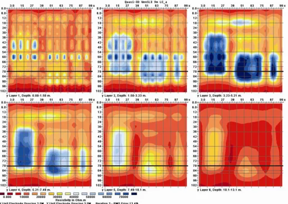
Fig. 2. Synthetic quasi-3-D image consisting of 20 forward modelled 2-D datasets arranged in x- and y-direction. The quasi-3-D image is based on the foreward model shown in Fig. 1b, including perpendicular profiles with the information of one single anomaly between 48 m and 93 m (x-direction), as shown in Fig. 4. Location of the transect shown in Fig. 4 is indicated by the bold black line.

(19)

TCD

3, 895–918, 2009

C. Kneisel et al.

Title Page

Tables Figures

◭ ◮

Back Close

Full Screen / Esc

‐ ‐

‐

Fig. 3. Synthetic quasi-3-D image consisting of 20 forward modelled 2-D datasets arranged in x- and y-direction. The quasi-3-D image is based on the foreward model shown in Fig. 1b, including perpendicular profiles with the information of a divided anomaly between 48 m and 93 m (x-direction), as shown in Fig. 5. Location of the transect shown in Fig. 5 is indicated by the bold black line.

(20)

TCD

3, 895–918, 2009

C. Kneisel et al.

Title Page

Tables Figures

◭ ◮

Back Close

Full Screen / Esc

‐

(21)

TCD

3, 895–918, 2009

C. Kneisel et al.

Title Page

Tables Figures

◭ ◮

Back Close

Full Screen / Esc

‐

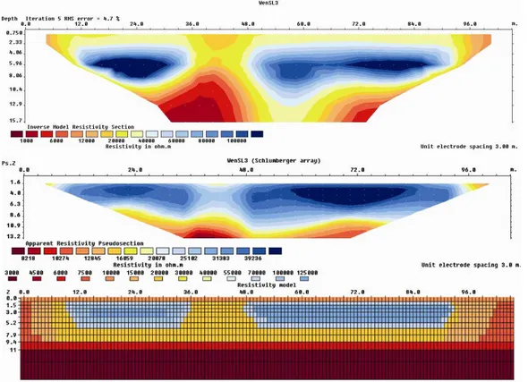
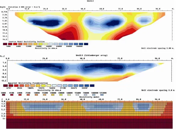
Fig. 5. Example of a synthetic 2-D cross profile (tie line) used to build up the quasi-3-D image of Fig. 3, with the input data of the forward model at the bottom, the resulting starting model in the middle and the inverted model at the top of the figure.

(22)