Comparison between three implementations of automatic identification algorithms for the quantification and characterization of mesoscale eddies in the South Atlantic Ocean

www.ocean-sci.net/7/317/2011/ doi:10.5194/os-7-317-2011

© Author(s) 2011. CC Attribution 3.0 License.

Ocean Science

Comparison between three implementations of automatic

identification algorithms for the quantification and characterization

of mesoscale eddies in the South Atlantic Ocean

J. M. A. C. Souza, C. de Boyer Mont´egut, and P. Y. Le Traon

Institut Franc¸ais de Recherche pour l’Exploitation de la Mer, Brest, France Received: 16 February 2011 – Published in Ocean Sci. Discuss.: 15 March 2011 Revised: 11 May 2011 – Accepted: 13 May 2011 – Published: 18 May 2011

Abstract. Three methods for automatic detection of mesoscale coherent structures are applied to Sea Level Anomaly (SLA) fields in the South Atlantic. The first method is based on the wavelet packet decomposition of the SLA data, the second on the estimation of the Okubo-Weiss pa-rameter and the third on a geometric criterion using the winding-angle approach. The results provide a comprehen-sive picture of the mesoscale eddies over the South Atlantic Ocean, emphasizing their main characteristics: amplitude, diameter, duration and propagation velocity. Five areas of particular eddy dynamics were selected: the Brazil Current, the Agulhas eddies propagation corridor, the Agulhas Cur-rent retroflexion, the Brazil-Malvinas confluence zone and the northern branch of the Antarctic Circumpolar Current (ACC). For these areas, mean propagation velocities and am-plitudes were calculated. Two regions with long duration eddies were observed, corresponding to the propagation of Agulhas and ACC eddies. Through the comparison between the identification methods, their main advantages and short-comings were detailed. The geometric criterion presents the best performance, mainly in terms of number of detections, duration of the eddies and propagation velocities. The results are particularly good for the Agulhas Rings, which have the longest lifetimes of all South Atlantic eddies.

1 Introduction

Oceanic eddies have been the subject of many experimental and theoretical studies in the last 40 yr. This is explained by the dominance of the kinetic energy associated to the

Correspondence to:J. M. A. C. Souza ([email protected])

mesoscale activity, more than one order of magnitude greater than that of the mean flow over most of the world ocean (Richardson, 1983; Chelton et al., 2007).

In the South Atlantic, in particular, the mesoscale activity is believed to play central roles in the southward heat flux in high latitudes (e.g., de Szoeke and Levine, 1981; Olbers et al., 2004; Mazllof et al., 2010) and the inter-ocean water properties exchanges with the Indian Ocean (e.g., de Ruijter et al., 1999; Matano and Beier, 2003; Sebille et al., 2010) and the North Atlantic Ocean (e.g., Fratantoni and Glickson, 2002; Jochum and Malanotte-Rizzoli, 2003; Ffield, 2005). Moreover, as presented by Wunsch (1999), eddy-induced heat fluxes have been observed to be important in western boundary current regions in the North Atlantic and Pacific Oceans. The role played by such structures in properties transport in the Brazil Current is not completely clear.

In the South Atlantic Ocean, most eddy variability stud-ies have been focused in the Agulhas Current Retroflection Rings (Fu and Zlotnicki, 1989; Gordon et al., 1992; Doglioli et al., 2007) and the Brazil-Malvinas Confluence (Goni et al., 1996; Fu, 2007). Although the existence of global estimates, as in Chelton et al. (2007, 2011), there is not yet a compre-hensive assessment of the eddies identification and tracking focused in the South Atlantic basin.

The South Atlantic presents optimal characteristics to test implementations of automatic eddy identification algorithms. The occurrence of high variability areas, such as the Agul-has Current retroflection and the Brazil-Malvinas confluence, corridors of eddies propagation, western boundary currents and the strongest current system in the world, the Antarctic Circumpolar Current (ACC), represent important obstacles to the correct identification and tracking of the structures.

With this in mind, several methods have been proposed for the identification and tracking of mesoscale structures in the ocean circulation. Classically, such methods can be divided into two main groups: one based on physical properties of the flow and other based in geometric criteria.

Physical properties can be difficult to estimate. Since they are often related to gradients of the measured sea prop-erties, errors inherent to the gradient estimations can have major impact on the final result. Moreover, the establish-ment of thresholds are necessary to determine the eddy lo-cations. Small variations of the thresholds values can have a profound impact on the number and location of the iden-tified structures. One of the most popular methods of this group is based on the Okubo-Weiss parameter (Okubo, 1970; Weiss, 1991). This method have been applied to both satellite data and numerical model results with considerable success (Isern-Fontanet et al., 2006; Chelton et al., 2007; Henson and Thomas, 2008). A modern alternative method for the detection of eddies using the wavelet analysis was proposed by Doglioli et al. (2007), based on the work of Siegel and Weiss (1997). This method consists in the decomposition of the sea surface relative vorticity into orthogonal modes, or wave packets, that are well localized in both position and wave number. The authors applied the method to the Cape Basin and compared the results with those obtained through the Okubo-Weiss parameter.

Although the use of geometric criteria is less usual than the physical ones, recent work have shown significant success in the identification of mesoscale vortex structures (Penven et al., 2005; Moolani et al., 2006; Chaigneau et al., 2008, 2009). Such methods assume that eddies consist in quasi-circular flow patterns, so the shape of instantaneous streamlines can be used for the structure identification. To achieve this objec-tive, two main techniques can be applied: the “curvature cen-ter method” (Leeuw and Post, 1995) and the “winding-angle method” (Sadarjoen and Post, 2000). The first approach is to locate the eddies by determining the center of the cur-vatures in the stream-lines. It presents the same problems associated to other point-based methods, with the identifi-cation of false peaks that have to be removed through the use of thresholds or filtering. As demonstrated by Sardojoen and Post (2000) and Chaigneau et al. (2008), the winding-angle method arrives to better results than the curvature cen-ter method, and was selected to represent the geometric cri-teria in the present study.

Chelton et al. (2011) proposed a threshold-free identifica-tion method, based on the Sea Surface Heigh (SSH) closed contours. This method is similar to the one implemented by Chaigneau et al. (2009) and used in the present study. The term “threshold-free“ refers to the fact that no especific SSH value is choosed to represent the eddy boundaries, although limits are imposed to the eddy amplitudes and diameters. While Chelton et al. (2011) made a global estimative of the eddies trajectories, the present study is focused in the South Atlantic region and the comparison between methods.

Con-trasting the results it is possible to identify how the differ-ences between this to similar methods impact the obtained eddy statistics.

The objective of the present work is to quantify and char-acterize the mesoscale coherent structures, or eddies, in the South Atlantic Ocean through the implementation of 3 dif-ferent methods for their automatic detection. These methods consist in (1) the estimation of the Okubo-Weiss parameter, (2) the Wavelet analysis of the sea surface relative vorticity and (3) the geometric winding-angle criterion. A comparison between the algorithms results will help to enlighten their ap-plicabilities and weaknesses, providing a valuable contribu-tion for future work.

In the next section the dataset used to the eddies detection is presented, together with the processing and simplifications adopted. The eddy identification and tracking algorithms are presented in the Sect. 3, followed by a comparison of their results in Sect. 4. Some conclusions are drawn in the Sect. 5, with propositions for future work.

2 Data

The domain of the present study corresponds to the South Atlantic Ocean, between the meridians of 70◦W and 30◦E and the parallels of 15◦S and 50◦S.

For this region, Sea Surface Height (SSH) data from the AVISO delayed time reference product were obtained from http://www.aviso.oceanobs.com/, from January 2005 to December 2008. It corresponds to a merged satellite product, projected on a 1/3◦ horizontal resolution Merca-tor grid, in time intervals of 7 days (Le Traon et al., 2003; Pascual et al., 2006).

To extract the anomalies (Sea Level Anomalies – SLA) from the original data, local time means were subtracted from each grid point. A low pass filter (Hanning with a win-dow of 175 days) was used to remove seasonal and inter an-nual signals. This procedure was particularly important to eliminate the low frequency variations of the oceanic fronts positions. A lanczos filter was applied to eliminate variabil-ity with length scales larger than 1000 km. This filter offers the best performance in terms of reduction of aliasing, with-out compromising the sharpness of the gradients (Turkowski and Gabriel, 1990).

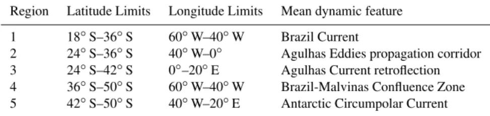
Fig. 1. Variance (cm2)of the SLA from AVISO over the years 2005 to 2008. Five areas of particular eddy dynamics are highlighted in white boxes: (1) The Brazil Current; (2) the corridor of propagation of Agulhas Eddies; (3) The Agulhas Current retroflection region; (4) the Brasil-Malvinas confluence zone and (5) the northern branch of the Antarctic Circumpolar Current.

Table 1.Limits between regions of particular eddy dynamics in the South Atlantic Ocean and their associated oceanographic features.

Region Latitude Limits Longitude Limits Mean dynamic feature

1 18◦S–36◦S 60◦W–40◦W Brazil Current

2 24◦S–36◦S 40◦W–0◦ Agulhas Eddies propagation corridor 3 24◦S–42◦S 0◦–20◦E Agulhas Current retroflection 4 36◦S–50◦S 60◦W–40◦W Brazil-Malvinas Confluence Zone 5 42◦S–50◦S 40◦W–20◦E Antarctic Circumpolar Current

3 Eddy identification and tracking algorithms

Three methods were applied for the identification of mesoscale eddies in the SLA data: the Okubo-Weiss param-eter, the wavelet analysis of the relative vorticity field and the geometry of the streamlines.

Surface eddy velocities and relative vorticity needed to be estimated for the application of the algorithms. Surface eddy velocities can be obtained from the SLA data through the geostrophic approximation (1):

v=

g

f ∂η

∂x u= −

g

f ∂η

∂y (1)

where (u,v) are the zonal and meridional surface eddy ve-locity components,ηis the SLA,gis gravity andf the Cori-olis factor. The relative vorticity (ω) can be than calculated, together with the normal (sn)and shear (ss)components of strain:

ω=∂v

∂x− ∂u

∂y sn= ∂u

∂x− ∂v

∂y

ss=

∂v

∂x+ ∂u

∂y (2)

After the identification of the eddies, the tracking of the structures was made through a algorithm based on the ideas presented in the study of Penven et al. (2005), and discussed in the end of this section.

3.1 Okubo-Weiss parameter

The Okubo-Weiss parameter (W ) was developed in the works of Okubo (1970) and Weiss (1991) and applied to sev-eral regions of the world ocean, both to satellite data and numerical model results. It is a method that aims to iden-tify regions in a flow were the relative vorticity dominates over the strain tensors, defined as the center of the eddy. The parameter is obtained by:

W=s_n2+s_s2−ω2 (3) Through W, the topology of the sea surface velocities can be divided into three types of regions (McWillians, 1984; Elhmaidi et al., 1993; Isern-Fontanet et al., 2006): ellip-tic regions (W <−W0), hyperbolic regions (W > W0)and

the background field (|W|< W0), where W0is a threshold

magnitude. The eddy core is defined as a region of negative

W (vorticity dominates over strain) surrounded by a region of positive W (strain dominates over vorticity). The back-ground field presents small magnitudes of W when com-pared to the eddies cores. Following previous work (Pas-quero et al., 2001; Isern-Fontanet et al., 2006; Henson and Thomas, 2008), the threshold was defined asW0=0.2σW,

σW being the spatial standard deviation of W with the

gives results very close to those obtained by simply defining

W0=−2×10−12s−2 as the eddies cores contours, as in

Chelton et al. (2007).

The noise in the resulting fields ofW difficult the iden-tification of the coherent structures. To overcome this, we applied a low pass spatial filter with a cut length scale of 50 km. Some results from the unfiltered fields of the Okubo-Weiss parameter are presented, in order to access the influ-ence of the filtering process. Unless otherwise posted, the results from the Okubo-Weiss parameter correspond to the filtered fields.

3.2 Wavelet analysis

The identification method based on the wavelet packet anal-ysis was proposed by Doglioli et al. (2007), inspired by the original work by Siegel and Weiss (1997). We applied a ver-sion of the routines developed by these authors (WATERS) for the analysis of numerical model results, and modified for the identification of structures in relative vorticity fields de-rived from satellite SLA data. The method resides in an em-pirical observation by Farge et al. (1992) and Wickerhauser et al. (1994) that coherent vortices in 2D turbulence can be ex-plained through a small number of the largest wavelet packet coefficients. The wave packets are than used to decompose the SLA derived vorticity maps and extract localized struc-tures in space.

The algorithm can be divided in five steps:

1. a best basis is chosen that minimize the Shannon en-tropy of the original field;

2. the surface relative vorticity is expanded on this basis; 3. the wavelets are sorted out as a function of their

coeffi-cients, where only the 10 % largest coefficients are kept. In fact, the number of coefficients kept is a critical pa-rameter of the analysis. The 10 % limit is based both in a series of tests and the bibliography (Doglioli et al., 2007; Rubio et al., 2009);

4. the structures are identified by the maximum of the vor-ticity modulus encircled by minimum vorvor-ticity regions; 5. structures with more than six grid cells in common are

merged to eliminate filaments.

3.3 Geometric criterion

This approach is supported by the statement by Robinson (1991):

“A vortex exists when instantaneous streamlines mapped onto a plane normal to the vortex core exhibit a roughly cir-cular or spiral pattern (. . . )”

Through this method, the SLA contours are used to detect the eddies with a modified winding-angle algorithm (Sadar-joen and Post, 2000). The eddy is defined by a maximum

SLA modulus, corresponding to the eddy center, encircled by a closed contour, the eddy edge. In the present study, we applied the algorithm described by Chaigneau et al. (2009).

The eddy identification process is performed in each time step, or SLA map, through two stages: (1) the identification of local SLA modulus maximum corresponding to the eddy centers and (2) the selection of closed SLA contours associ-ated to each eddy. The outermost contour embedding only one eddy center is considered as the eddy edge. This method is very similar to the one applied by Chelton et al. (2011), and showed a good performance in terms of processing time when compared to other classical methods.

3.4 Eddy amplitudes and diameters

For the characterization of the eddies and comparison be-tween algorithms, eddy diameters and amplitudes were com-puted. The eddy diameter was defined as the equivalent di-ameter (De)of a circle with the same area (A)as the closed contour delimitating the eddy borders Eq. (4).

De=2

r

A

π (4)

The amplitude is defined as the difference between the max-imum of the SLA modulus inside the eddy and the modulus of the SLA at the border.

Eddies with diameters smaller than 50 km were ignored. In fact, real eddies smaller than this threshold are not cor-rectly resolved in the SLA grid.

3.5 Tracking algorithm

The same tracking algorithm was used for the three identifi-cation methods. The eddies central points were determined by the maximum SLA modulus. After identification, the cen-tral points were tracked in time minimizing a dissimilarity parameter Eq. (5) proposed by Penven et al. (2005).

Xe1,e2= s _1X X0 2 + _1R R0 2 + _1ξ ξ0 2 (5) where1Xis the distance between the eddiese1ande2

cen-ters,1Ris the diameter difference and1ξ the vorticity dif-ference. X0is a characteristic length scale (1000 km),R0a

characteristic diameter (100 km) andξ0a characteristic

vor-ticity (10−6_s−1_{). The parameter was calculated for all eddies}

identified in each time step (e1), in relation to the eddies in

the subsequent time step (e2)which centers are less than 2◦

distant and that have the same vorticity sign.

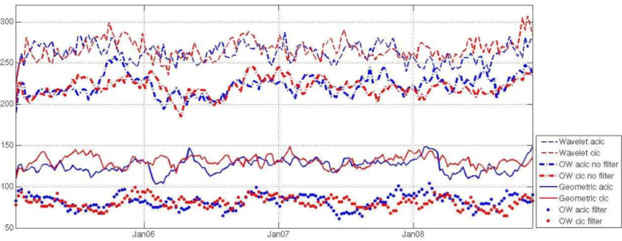
Fig. 2. Total number of eddies present in the South Atlantic between 70◦W–30◦E and 50◦S–15◦S, obtained from the three automatic identification algorithms, as a function of time. The colors indicate the occurrence of anti-cyclonic (blue) and cyclonic (red) eddies. The impact of the filtering process in the Okubo-Weiss method can be observed through the reduction in the number of observed structures.

Fig. 3.Total number of identified eddies per grid point for the three automatic identification algorithms, normalized by the maximum number of identifications.

for another 2 time steps (14 days). This helped avoiding loos-ing track of the eddies as consequence of problems with the interpolation of the along track altimetry to a regular grid.

Eddies with lifetimes shorter than four weeks were re-moved from the analysis.

4 Results and discussions 4.1 Mean properties

We first compare the results from the three identification methods in terms of the mean eddy properties. As mean properties we understand the number of identified structures, their mean diameters and durations.

The total numbers of identified eddies with lifetimes larger than 4 weeks, for each method, are showed in Fig. 2. Al-though the Okubo-Weiss method have been reported to have a high number of false identifications (Isern-Fontanet et al., 2006; Chaigneau et al., 2008), the wavelet analysis yields the higher number of identifications. No predominance of cyclonic or anti-cyclonic eddies is observed through any method.

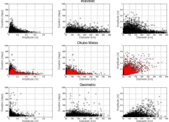
Fig. 4.Relations between the mean characteristics (duration, amplitude and diameter) of all anti-cyclonic eddies obtained through the three identification algorithms. In the Okubo-Weiss method results, the black points indicate the unfiltered and the red points the filtered results.

The high number of identified structures for the Wavelet analysis method, spread all over the domain, can be associ-ated to a difficulty of dealing with regions of very different SLA variances. Indeed, one of the hypothesis of the Siegel and Weiss (1997) work is the isotropy of the eddy field. So, it can be speculated that the observed over-identification is a consequence of the wavelet coefficients sorting. When try-ing to retain only the 10 % larger coefficients in such an het-erogeneous area, the method ends up by overestimating the presence of eddies in the less active parts of the analysis do-main. This would explain the relative homogeneous spatial distribution of the number of identifications. Actually, pvious work have applied the wavelet method to restricted re-gions, such as the Cape Basin (Doglioli et al., 2007) and the Benguela upwelling system (Rubio et al., 2009).

The number of eddies tracked in the Okubo-Weiss algo-rithm is highly sensitive to the thresholdW0 and the

filter-ing process. As reported by Chelton et al. (2007), smaller values of W0 results in a larger number of eddies tracked

in regions of small SLA variance, but reduces the number of eddies tracked in regions of high SLA variance. When dealing with very heterogeneous regions, such as the South Atlantic, a compromise or mean threshold value has to be chosen. Also, the filtering process has an important impact in the number of structures in the Okubo-Weiss method with more than 50 % of reduction in the number of identifications. If on one hand the filter reduces the number of false

identi-fications caused by small noisy structures, on the other hand it reduces the capability of the method to keep track of the structures for a long period of time. Nevertheless, the filter-ing is necessary to avoid the noise to contaminate the mean diameter and duration statistics.

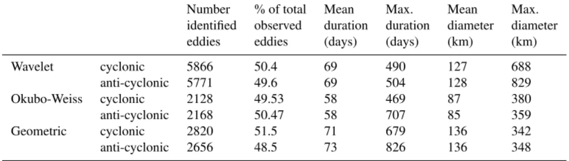
The total numbers of identified eddies, their diameters and durations are presented in Table 2. This table shows that the Okubo-Weiss method results in mean diameters∼35 % smaller than the other two identification algorithms. Indeed, Henson and Thomas (2008) have reported a∼50–60 % un-derestimation of eddy core diameters using the Okubo-Weiss parameter in the Gulf of Alaska. The smaller difference in the present work should be a function of the more hetero-geneous area, the filtering process and the value of theW0

threshold. One should observe that the maximum diameters obtained through this method are very similar to the results from the other two algorithms. This indicates that the under-estimation of diameters by the Okubo-Weiss parameter is not homogeneous.

Table 2.Eddy properties obtained from the three automatic identification algorithms.

Number % of total Mean Max. Mean Max. identified observed duration duration diameter diameter eddies eddies (days) (days) (km) (km)

Wavelet cyclonic 5866 50.4 69 490 127 688

anti-cyclonic 5771 49.6 69 504 128 829

Okubo-Weiss cyclonic 2128 49.53 58 469 87 380

anti-cyclonic 2168 50.47 58 707 85 359

Geometric cyclonic 2820 51.5 71 679 136 342

anti-cyclonic 2656 48.5 73 826 136 348

Fig. 5.Relations between the mean characteristics (duration, amplitude and diameter) of all anti-cyclonic eddies obtained from the Chelton et al. (2011) results in the same region and period of the present study.

to the loss of energy (amplitude) with lifetime observed for the long living structures. As an example, Byrne et al. (1995) estimated that the Agulhas Rings reach 40◦W with∼10 % of their original amplitude.

The relation between duration and diameter is not so clear. Although the Okubo-Weiss results shows that the larger du-ration eddies have mean diameters of approximately 100– 150 km, the same is not clear in the geometric criterion and Wavelet analysis results. This is particularly true for the anti-cyclonic eddies, where the geometric criterion method shows highly variable long living eddies mean diameters.

Similarly, it is possible to observe a tendency of mean amplitude increase with the mean diameter increase in the Okubo-Weiss and geometric criteria results, although the small amplitude eddies present a large range of mean diameters.

The filtering process does not have an important impact in the properties relations in the Okubo-Weiss method. How-ever, some of the longer duration structures are lost due to the filter. This is of great interest when trying to track partic-ular long living structures, as the Agulhas Rings.

The same eddy properties were calculated from the re-sults of Chelton et al. (2011), for the region and period of the present study (available at http://cioss.coas.oregonstate. edu/eddies/) and are presented in Fig. 5. The relations be-tween the amplitudes and the eddies durations and diameters follow the same pattern of the previous methods, althougth

the longer durations. A particular good agreement is oberved with the geometric method. Differently from the methods analysed in this work, the longer durations eddies tend to have diameters around 200 km. This can be a consequence of the dominance of the Agulhas Rings as the longer dura-tions structures in the South Atlantic, but further analysis is necessary to confirm this hypothesis.

The automated tracking algorithm is an important aspect that can be related to the longer duration of the eddies oberved by Chelton et al. (2011). The method applied by these authors uses a zonally oriented elliptical search area for the continuation of the eddies. The size of the ellipse is related to the velocity propagation of non-dispersive Rossby waves, with a minimum value of 150 km. A wide range of variation of the eddy properties is permitted between con-secutive time steps, without the estimation of the similarity. Although the fixed search area used in the present study does not take into account the variation of the eddy propagation velocities, the dissimilarity parameter promotes a better sep-aration between different structures.

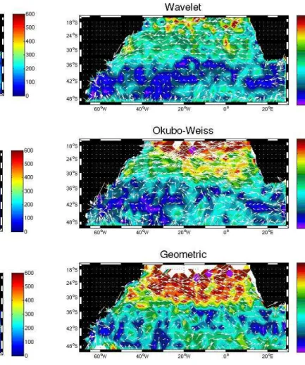
Fig. 6.Mean eddy equivalent diameters (km) in the formation mo-ment, as derived from the three identifications algorithms. The black contours indicate intervals of 50 km.

The same pattern is not observed in the Okubo-Weiss method results. In this algorithm the eddy diameters seem to be function of their energy, with larger eddies occurring in the Brazil-Malvinas confluence and the Agulhas retroflection – where higher SLA variability is observed (see Fig. 1).

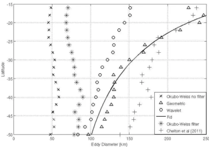
This difference between the three methods is demonstrated in the zonal mean eddies diameters in Fig. 7, where the re-sults obtained by Chelton et al. (2011) are also presented. In this figure, we observe that the eddies tracked through the ge-ometric criteria present a relation between the diameter and the latitude very close to the curve of the first baroclinic mode Rossby deformation diameter (Rd – two times the Rossby de-formation radius). This characteristic is reflected in the mean diameter presented in Table 2, with the geometric criterion results showing higher values. The wavelet analysis results show an almost linear relation between latitude and diameter, with a smaller inclination relative to Rd. The Okubo-Weiss zonal mean diameters are almost constant with latitude. Al-though the filtering of the Okubo-Weiss results eliminate the

Fig. 7.Zonal mean eddy diameters obtained from the three identi-fication algorithms and in Chelton et al. (2011). The solid line is a estimation of the first baroclinic mode Rossby deformation diame-ter (Rd).

smaller structures, the relation between diameter and latitude keeps unchanged.

The Chelton et al. (2011) results present diameters∼50 % larger in high latitudes (south of 30◦S) than the present study. This can be an influence of the Brazil-Malvinas convergence zone and the Agulhas Current retroflexion, since these au-thor results indicate the presence of large structures in these areas as a function of the presence of closed SSH contours. A similar characteristic is oberved for the Okubo-Weiss pa-rameter based method, generating a coincident bump in the mean diameters at 40◦S related to the Brazil-Malvinas con-fluence (Fig. 7). In fact, in Chelton et al. (2011) a maximum threshold of 400 km is established for the eddy diameters at this latitude. It can be argued that this value is too large to prevent a contamination from the confluence front position in the eddy identification results.

Fig. 8. Eddy lifetimes (days) at their birth points. The color con-tours indicate the duration of the identified eddies plotted in their first observation locations. The black contours represent intervals of 100 days.

It is interesting to observe that, for the three identification methods, the origin points of the Agulhas eddies are not ex-actly in the retroflexion. This is an indication that the eddies have been tracked only after detaching of the Agulhas Cur-rent. Similar results were obtained by Byrne et al. (1995) and Schonten et al. (2000) when tracking Agulhas Rings (anti-cyclonic eddies) in SLA satellite data, and by Chelton et al. (2011).

4.2 Propagation velocities

Using all the tracks from eddies with durations larger than 4 months, it was possible to generate maps of mean prop-agation velocities (Fig. 9). The geographical pattern ob-tained from the three methods are similar, presenting a zone of minimum velocities centered in 42◦S. From this mini-mum axis, velocities increase both to the north and to the south, with directions following the anti-clockwise

subtropi-Fig. 9.Mean propagation velocities (km day−1)for the eddies ob-tained from the three identification methods.

cal wind-driven circulation gyre. The eddies propagate west-ward through most the domain. The only exceptions are the ACC eddies, that are advected eastward by the strong mean flow as noted by Hughes et al. (1998).

Table 3. Mean eddy propagation velocities for the five areas of particular dynamics highlighted in Fig. 1, obtained from the results of the three identification methods.

Eddy propagation velocities (km day−1)

Region 1 Region 2 Region 3 Region 4 Region 5

Wavelet cyclonic 3.36 2.89 2.63 2.02 2.11

anti-cyclonic 3.26 3.04 2.43 1.99 2.02 Okubo-Weiss cyclonic 3.01 3.44 3.48 1.89 2.06 anti-cyclonic 2.68 3.5 3.21 1.88 2.04

Geometric cyclonic 3.98 4.88 3.61 2.69 2.99

anti-cyclonic 4.45 4.99 3.78 2.62 2.96

a space-time lagged correlation analysis to characterize the pathways and propagation velocities of eddies in the South Atlantic Ocean. However, comparisons must be done with care since this author considered all perturbations to the mean state as eddies, while the present study focuses on the coherent structures, or vortices. The zone of high veloci-ties observed by Fu (2006) in the Brazil-Malvinas confluence can be associate to short living eddies or other processes that are excluded from the present analysis. The same hypothesis can be made to the area of the Agulhas Current retroflection, where the method applied by Fu (2006) included the current meanders and the vortex structures before pinching off the retroflection.

Although similar in terms of distribution, the absolute val-ues of the velocities differ between the methods. The geo-metric criterion presented overall larger velocities than the other two. For a suitable comparison, mean values of veloci-ties in the five areas highlighted in the Fig. 1 where calculated (Table 3).

In fact, although the three methods mean propagation ve-locities are similar, an important exception is observed in the Agulhas eddies propagation corridor (Region 2). Pre-vious work has reported values of velocities for the Agul-has Rings (anti-cyclonic AgulAgul-has eddies) ranging between 3.71 km day−1_{(Byrne et al., 1995), 4.3–6.9 km day}−1

(Gor-don and Haxby, 1990), and 7–8 km day−1 (Garzoli et al., 1999). The velocities from the geometric criterion results (4.99 km day−1)are in the range of the bibliography, while the other two methods present smaller values.

Using the eddies tracks obtained by the geometric method as a reference, it was possible to observe that the other meth-ods were able to identify the same structures. Although the track lengths obtained through the Okubo-Weiss parameter and Wavelet analysis were shorter than those obtained by the geometric criteria, the mean propagation velocities were the same, as one would expect.

4.3 Long-lived eddies

The analysis presented to this point reflects the mean eddy behavior. Although this view provides an important compari-son between identification methods, it may hide some impor-tant differences relative to the long-lived structures. These eddies are of particular interest due to their important contri-butions to the eddy fluxes across the basin, their large partic-ipation in the total variance and particular role in the inter-basin water exchanges (Doglioli et al., 2007; Richardson, 2007; Sebille et al., 2010).

From the maps of Fig. 8, two regions of larger duration eddies where selected for further analysis. Only eddies with lifetimes larger than 120 days (∼4 months) were used to en-sure that all identified structures leave the formation region. The Agulhas eddy formation area was defined between the meridians of 0◦ and 20◦E and the parallels of 40◦S and 30◦S, while the Antarctic Circumpolar Current (ACC) ed-dies area was defined between the meridians of 20◦W and 0◦and the parallels of 50◦S and 40◦S. The eddy tracks orig-inated from these regions are presented in the Fig. 10 and the eddy mean characteristics in the Table 4.

The method based in the wavelet analysis and the filtered fields of Okubo-Weiss parameter were less efficient in track-ing the Agulhas Rtrack-ings (anti-cyclones) across the South At-lantic Basin. While the geometric criterion was able to keep track of several eddies farther than 30◦W, as done visually by Gordon and Haxby (1990), the Okubo-Weiss method had this level of success in only one occasion, without the appli-cation of the filter.

The “fragmentations” of the eddy tracks in the wavelet analysis method are consequence of failures of identification in three or more consecutive time steps, or more than the 14 days used to search for the tracks continuity. Such fragmen-tation is associated not only to the shorter observed tracks, but contribute also to the homogeneous distribution of iden-tifications relative to the other methods (see Fig. 3) and to the higher total number of structures.

Table 4.Long-lived eddy properties obtained from the three identification algorithms. In the Okubo-Weiss results, the upper (lower) lines refer to the filtered (unfiltered) results.

N. Mean Max. Mean Max. Mean Max. ident. dur. dur. Amp. Amp. diam. diam. (days) (days) (m) (m) (km) (km)

Wavelet Agulhas cyclonic 54 170 294 0.09 0.27 137 431 anti-cyclonic 50 193 448 0.11 0.61 142 418

ACC cyclonic 83 183 434 0.06 0.19 119 448

anti-cyclonic 94 1674 462 0.05 0.19 112 348

Okubo-Weiss Agulhas cyclonic 07 153 224 0.11 0.19 92 133

33 169 392 0.09 0.56 61 150

anti-cyclonic 17 224 448 0.13 0.37 102 177

43 228 896 0.09 0.44 71 168

ACC cyclonic 19 147 196 0.09 0.19 92 172

88 183 686 0.05 0.16 51 125

anti-cyclonic 9 157 203 0.08 0.23 100 163

82 173 462 0.05 0.15 58 151

Geometric Agulhas cyclonic 43 146 252 0.1 0.42 155 319 anti-cyclonic 40 295 826 0.09 0.59 156 289

ACC cyclonic 58 194 483 0.04 0.14 121 237

anti-cyclonic 44 174 518 0.04 0.14 124 200

results, the filtering process presented an important impact in the reduction of the number of tracked structures, their dura-tions and diameter. Although the filtering prevents the track-ing of small structures, it clearly reduces the efficiency in keeping track of the longer living eddies that crosses the At-lantic Basin. The same was observed by Chelton et al. (2011) when comparing the results to their previous work (Chelton et al., 2007), where the Okubo-Weiss parameter was used.

Considering only the Agulhas Rings that cross the 0◦ meridian in the geometric method results, leaving the for-mation region, approximately 4.5 eddies were observed to be shed each year. Such rings present a mean diameter of 166 km. These results are in agreement with the literature, which propose that a ring is typically shed from the Agul-has retroflection every 2–3 months with a typical diameter of 150–200 km (Byrne et al., 1995; Beismann et al., 1999; Schonten et al., 2000; Van Aken et al., 2003; de Steur et al., 2004; Doglioli et al., 2007).

For the Agulhas cyclones, the results exhibit a large vari-ation between the number of identified structures by each method. These cyclones are believed to play a important, though secondary, role in the inter-basin ocean waters ex-change. They have been reported to travel southwestward into the South Atlantic and trigger the pinching off of Agul-has Rings (Lutjeharms et al., 2003). The trajectories repre-sented in Fig. 10 show that most cyclonic eddies do not leave the proximity of the Cape Basin. Even those that follow a westward trajectory similar to the anti-cyclones do not have their longevity, never reaching longitudes west of 10◦W. In

fact, Boebel et al. (2003) revealed that the Cape Basin off Cape Town is filled with Agulhas Rings and cyclonic ed-dies interacting with each other, and a similar behavior is ob-served through the trajectories obtained in the present work. As described by Matano and Beier (2003), the Agulhas cy-clone mean diameters were observed to be generally smaller than the anti-cyclones.

Despite the short time period of four years used, it is pos-sible to observe a seasonal variability in the formation of the long-living Agulhas anti-cyclonic eddies (Fig. 11). There is a higher number of Agulhas Rings formed in the summer and winter months, with a detached participation of the month of December. The same is not observed for the cylones, that presented more homogeneous formation rates along the year. In the ACC eddies formation region, both the cyclonic and anti-cyclonic eddies show very diffuse tracks. In general, ed-dies present a eastward propagation following the main flow. This is better evidenced in the geometric criterion and fil-tered Okubo-Weiss parameter results. In fact, the ACC was the only region where Chelton et al. (2011) were able to iden-tify long-living (>16 weeks) eastward propagating eddies in the southern hemisphere.

Fig. 10.Track of the long-lived eddies (duration>12 weeks) origi-nated in the Agulhas retroflection (northeastern black rectangle) and Antarctic Circumpolar Current (southwestern black rectangle). The blue lines indicate cyclonic and the red lines anti-cyclonic eddies.

It is important to emphasize that the ACC eddy formation re-gion defined in the present study refers only to the larger du-ration structures observed in the South Atlantic. Eddies that enter the Atlantic basin through the Drake passage or leave the basin to the east have their lifetimes underestimate due to the domain restrictions.

Fig. 11. Number of Agulhas eddies formed per month in the years 2005 to 2009. It corresponds to the long-lived eddies with durations higher than 120 days and that cross the 0◦meridian, leaving the formation region.

The eddies in the ACC region are smaller and less intense than in the Agulhas region (Table 4). As observed in the mean results, the Wavelet analysis presented a higher number of structure identification, followed by the unfiltered Okubo-Weiss parameter. The underestimation of the eddy diame-ters by the Okubo-Weiss parameter is also reproduced in this case. In opposition to the Agulhas eddies, there is no clear difference between the ACC cyclonic and anti-cyclonic eddy track lengths in Fig. 10. While the mean eddy durations ob-tained for the three methods are similar, the maximum values presented important differences. Again, the wavelet analysis present the smaller lifetimes. Although the maximum dura-tion value for a cyclone in the ACC region is detected with the Okubo-Weiss parameter, it represents an isolated case where the method merged two subsequent structures. Sim-ilarly to the Agulhas Rings, the ACC anti-cyclones presented a seasonal cycle in the formation rate. The same is not truth for the cyclones (Fig. 12).

As noted by Morrow et al. (2004) and Chelton et al. (2011), the anti-cyclones present a small northward de-flection in their propagation direction. This tendency is more clear in the Agulhas Rings than in the ACC eddies. Although the expected southward deflections of the cyclones trajecto-ries are not clear in the results obtained by any method, the difference from the anti-cyclones pattern is notable. This should be a consequence of the shorter duration of the cy-clones resolved by the identification and tracking algorithms.

4.4 Agulhas Rings decay

Fig. 12. Number of ACC eddies formed per month in the years 2005 to 2009. It corresponds to the long-lived eddies with durations higher than 120 days.

Fig. 13.Amplitude of Agulhas eddies as a function of the distance from their first identification site. The ( (

.

in the bibliography (Byrne et al., 1995; Sebille et al., 2010). Such characteristic were not observed for the eddies origi-nated in the ACC region. All the observed long-lived Agul-has rings were used in the present estimates.

The three identification methods give similar eddy decay results (Fig. 13). Despite the differences in eddy durations, the exponential character described by Byrne et al. (1995) is observed for the anti-cyclones (Agulhas Rings). The authors have calculated a 81 % amplitude reduction for the Agulhas Rings during its life. The present results show that, based in the geometric criterion, an 83 % amplitude reduction should be expected for a typical Agulhas Ring between its origin and end of lifetime.

Although the exponential decay relation observed in Fig. 11, a linear fit can be used to estimate the mean de-cay rate of a typical Agulhas Ring (Fig. 14). The geometric criterion results were selected for showing a larger number of eddies with long durations. The mean decay rate obtained

Fig. 14. Amplitude decay for a mean Agulhas Ring tracked through the geometric criterion. The red line is a linear fit with a −9.33×10−5m day−1angular coefficient.

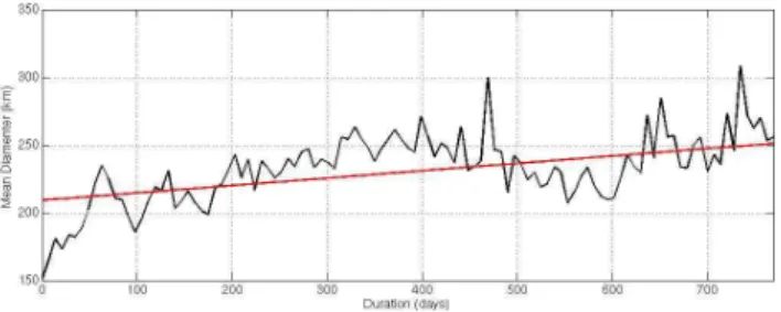
Fig. 15. Diameter modification of a mean Agulhas Ring tracked through the geometric criterion. The red line is a linear fit with a 5.45×10−2km day−1angular coefficient.

indicates a reduction of 9.33×10−5m day−1in the eddy am-plitudes. Similarly, a modification in the eddies diameter is observed along their lifetime. Through the linear fit, a rate of 5.54×10−2km day−1 diameter increase was calculated (Fig. 15).

4.5 Time variability

The regions of particular eddy dynamics, highlighted in Fig. 1, were used to study the time variability of the eddy characteristics obtained through the three identifica-tion methods. Since all eddies identified were included in the analysis, the results include the influence of the different number of eddies obtained by each method.

Fig. 16.Mean eddy amplitudes (m) for five areas of particular high SLA variance in the South Atlantic Ocean. Note the amplitude scales are different between the figures due to the distinct values presented by the regions. The blue lines ( ( )) indicate the results from the Wavelet analysis method, the red lines ( ( )) the results from the Okubo-Weiss parameter and the black lines (s ( ) t) the results from the geometric criterion.

Analyzing the spectra of the eddy amplitudes in the Fig. 17, it is possible to observe that the main variability fre-quencies are reproduced by the three methods. Larger dif-ferences in the spectral energy content occurs in the Agulhas eddies propagation area (Region 2) and the Brazil-Malvinas Confluence zone (Region 4). In the first case the difference can be explained by the larger number of long living eddies tracked through the geometric criterion. Indeed, a secondary spectral peak of 66 days in the Region 2 spectrum can be associated to the periodicity of the Agulhas Rings shedding, as this is the major feature influencing the SLA variability in this area.

A particularly good agreement between the spectra from the Wavelet analysis and the geometric criterion denotes a similarity between the behavior of the identified structures in both methods. From these results one can observe that, while region 2 is the only one that presents a dominating annual cycle, regions 4 and 5 show coherent peaks corresponding to the periods of 98 and 183 days.

The coincidence of the Region 5 (ACC) 183 day spectral peak in the three methods results is remarkable. This denotes the influence of a dominating mode of variability. Some

studies (e.g., Meredith et al., 2006; Thompson and Wallace, 2000; Thompson et al., 2000) relate the sub-seasonal vari-ability in the SLA field in the Southern Ocean to the South-ern Hemisphere Annular Mode. More analysis, which are beyond the scope of this study, are necessary to confirm this relationship.

5 Conclusions

Fig. 17.Eddy amplitude time spectra (m2)for five regions of particular high SLA variance in the South Atlantic Ocean. The blue lines ( ( )) indicate the results from the Wavelet analysis method, the red lines ( ( )) the results from the Okubo-Weiss parameter and the black lines (s ( ) t) the results from the geometric criterion.

It is interesting to observe that the three methods give similar number of cyclone and anti-cyclone identifications. Moreover, no inter-annual variation is observed in the num-ber of eddies between 2005 and 2008. This may be a conse-quence of:

1. the short time length of the SLA data used in the present study;

2. the number of eddies computed for the South Atlantic basin as a whole, masking local variations.

The areas of higher SLA variance could be related to the presence of coherent structures. The same pattern of geo-graphical distribution is observed in the map of SLA vari-ance (Fig. 1) and the number of identified eddies (Fig. 3) in the Okubo-Weiss parameter and geometric criterion results. However, a direct link between the SLA variance and number of eddies is not possible, since the variability in high energy areas is consequence of several different processes. This is particularly the case in the Agulhas Current retroflexion and the Brazil-Malvinas confluence, in the South Atlantic Ocean. Although the variance in these areas is considerably higher, the number of identified structures is similar to the Agul-has eddies corridor and the ACC. The identification method

based on the wavelet analysis could not retrieve the same ge-ographical pattern.

The geometric criterion presented the best performance in terms of eddy identification and tracking. The eddy char-acteristics from this identification method presented the bet-ter level of agreement with the other two algorithms and the bibliography. Particularly, eddy diameters show a good re-lationship with the first baroclinic mode Rossby deformation radius. Moreover, the time length and propagation velocities obtained through the geometric criterion are in close agree-ment with previous work.

Although the application of a spatial filter was necessary to remove small scale noisy structures from the Okubo-Weiss parameter results, it had serious consequences on the track-ing of the long livtrack-ing eddies. This is well manifested in the small number of Agulhas Rings tracked after filtering, and their short durations in comparison to the geometric crite-rion and the bibliography. The unfiltered parameter presents good results in terms of the duration of the eddies, but fails on represent their mean diameters and arrives to small values of propagation velocities.

The present results corroborate the hypothesis by Chelton et al. (2007) that most variability in the middle of the oceanic basins is associated with mesoscale coherent structures. In the South Atlantic such variability is strongly associated to the propagation of Agulhas eddies, with the anti-cyclones (Agulhas Rings) playing a leading role.

Other modern methods to identify coherent structures in turbulent flows have been suggested. As an example, Hua and Klein (1998) have proposed a method based in the La-grangian acceleration tensor, overcoming the Okubo-Weiss parameter deficiencies and better representing the flux topol-ogy in the case of decaying two-dimensional turbulence. Other method is based in the instantaneous Lagrangean flow geometry through the Lyapunov function (Haller, 2005). Al-though the potential benefits, there is no application to real oceanic eddies present in the peer reviewed literature.

Although the SLA data used in the present work permit-ted the surface localization and delimitation of the eddies, the lack of knowledge about their vertical structure presents a strong barrier in the estimation of their role in the oceanic heat and water masses fluxes. New global in-situ observa-tions, such as the ARGO profiling floats, should provide a means to better estimate their vertical structure. The com-bination of the eddies tracks obtained in the present study with vertical profiles should provide new estimations for the oceanic eddy fluxes and will be addressed in future work.

Acknowledgements. The authors would like to thank Nico-las Grima and Alexis Chaigneau for providing the WATERS (wavelet packet method) and the geometric criterion routines. Spe-cial thanks to Luiz Alexandre Guerra for the ideas and discussions on the Agulhas Rings. Joao Marcos Souza is funded through a IFREMER postdoctorade fellowship.

Edited by: M. Hecht

References

Beismann, J. O., Kase, R. H., and Lutjeharms, J. R. E.: On the influ-ence of submarine ridges on propagation and stability of Agulhas rings, J. Geophys. Res., 104, 7897–7906, 1999.

Boebel, O., Lutjeharms, J., Schmid, C., Zenk, W., Rossby, T., and barron, C.: The Cape Cauldron: A regime of turbulent inter-ocean exchange, Deep-Sea Res. II, 50, 57–86, 2003.

Byrne, D. A., Gordon, A. L., and Haxby, W. F.: Agulhas eddies: A synoptic view using Geosat ERM data, J. Phys. Oceanogr., 25, 902–917, 1995.

Chaigneau, A., Gizolme, A., and Grados, C.: Mesoscale eddies off Peru in altimeter records: Identification algorithms and eddy spatio-temporal patterns, Prog. Oceanogr., 79, 106–119, 2008. Chaigneau, A., Eldin, G., and Dewitte, B.: Eddy activity in the four

major upwelling systems from satellite altimetry (1992–2007), Prog. Oceanogr., 83, 117–123, 2009.

Chelton, D. B., Schlax, M. G., Samelson, R. M., and de Szoeke, R. A.: Global observations of large oceanic eddies, J. Geophys. Res., 34, L15606, doi:10.1029/2007GL030812, 2007.

Chelton, D. B., Schlax, M. G., and Samelson, R. M.: Global Ob-servations of Nonlinear Mesoscale Eddies. Prog. Oceanogr., in press, doi:10.1016/j.pocean.2011.01.002, 2011.

De Ruijter, W. P., Biastoch, A., Drijfhout, S. S., Lutjeharms, J. R. E., Matano, R. P., Pichevin, T., Van Leeuwen, P. J., and Weijer, W.: Indian-Atlantic interocean exchange: Dynamics, estimation and impact. J. Geophys. Res., 104(C9), 20885–20910, 1999. De Steur, L., Van Leeuwen, P. J., and Drijfhout, S. S.: Tracer

leak-age from modeled Agulhas rings, J. Phys. Oceanogr., 34, 1387– 1399, 2004.

De Szoeke, R. A. and M. D. Levine: The advective flux of heat by mean geostrophic motions in the Southern Ocean, Deep-Sea Res. I, 28A, 1057–1085, 1981.

Doglioli, A. M., Blanke, B., Speich, S., and Lapeyre, G.: Tracking coherent structures in a regional ocean model with wavelet anal-ysis: Application to Cape Basin eddies. J. Geophys. Res., 112, C05043, doi:10.1029/2006JC003952, 2007.

Elhmaidi, D., Provenzale, A., and Babiano, A.: Elementary topol-ogy of two-dimensional turbulence from a Lagrangian viewpoint and single-particle dispersion. J. Fluid Mech., 257, 533–558, 1993.

Farge, M. E., Goirand, Y., Meyer, Y., Pascal, F., and Wicker-hauser, M. V.: Improved predictability of two-dimensional tur-bulent flows using wavelet packet compression, Fluid Dyn. Res., 10, 229–250, 1992.

Ffield, A.: North Brazil Current rings viewed by TRMM Mi-crowave Imager SST and the influence of the Amazon Plume, Deep-Sea Res. I, 52, 137–160, 2005.

Fratantoni, D. M. and Glickson, D. A.: North Brazil Current Ring generation and evolution observed with SeaWifs, J. Phys. Oceanogr., 32, 1058–1074, 2002.

Fu, L. L. and Zlotnicki, V.: Observing oceanic mesoscale eddies from Geosat altimetry: Preliminary results, Geophys. Res. Lett., 16, 457–460, 1989.

Fu, L. L.: Pathways of eddies in the South Atlantic Ocean revealed from satellite altimeter observations, Geophys. Res. Lett., 33, L14610, doi:10.1029/2006GL026245, 2006.

Fu, L. L.: Interaction of mesoscale variability with large-scale waves in the Argentine Basin, J. Phys. Oceanogr., 37, 787–793, 2007.

Gallego, B., Cessi, P., and McWilliams, J. C.: The Antarctic Cir-cumpolar Current in Equilibrium, J. Phys. Oceanogr., 34, 1571– 1587, 2004.

Garzoli, S. L., Richardson, P. L., Duncombe Rae, C. M., Fratantoni, D. M., Goni, G. J., and Roubicek, A. J.: Three Agulhas Rings observed during the Benguela Current Experiment, J. Geophys. Res., 104(C9), 20971–20985, 1999.

Goni, G., Kamhols, S., Garzoli, S., and Olson, D.: Dynamics of Brazil-Malvinas Confluence based on inverted echo sounders and altimetry, J. Geophys. Res., 101(C7), 16273–16289, 1996. Gordon, A. L. and Haxby, W. F.: Agulhas eddies invade the

South Atlantic: Evidence from Geosat altimeter and ship-board conductivity-temperature-depth survey, J. Geophys. Res., 95(C3), 3117–3125, 1990.

Gordon, A. L., Weiss, R. F., Smethie Jr., W. M., and Warner, M. J.: Thermocline and intermediate water communication between the South Atlantic and Indian Oceans, J. Geophys. Res., 97, 7223– 7240, 1992.

1–26, 2005.

Henson, S. A. and Thomas, A. C.: A census of oceanic anticy-clonic eddies in the Gulf of Alaska, Deep-Sea Res. I, 55, 163– 176, 2008.

Hua, B. L. and Klein, P.: An exact criterion for the stirring proper-ties of nearly two-dimensional turbulence, Physica D, 113, 98– 110, 1998.

Hughes, C. W., Jones, M. S., and Carnochan, S.: Use of Transient Features to Identify Eastward Currents in the Southern Ocean, J. Geophys. Res. (Oceans), 103(C2), 2929–2944, 1998.

Isern-Fontanet, J., Garcia-Ladona, E., and Font, J.: Vortices of the Mediterranean Sea: An altimetric perspective. J. Phys. Oceanogr., 36, 87–103, 2006.

Jochum, M. and Malanotte-Rizzoli, P.: On the generation of North Brazil Current Rings, J. Mar. Res., 61, 147–162, 2003.

Karsten, R. H. and Marshall, L.: Constructing the residual Circu-lation of the ACC from Observations. J. Phys. Oceanogr., 32, 3315–3327, 2002.

Le Traon, P. Y., Faug`ere, Y., Hernandez, F., Dorandeu, J., Mertz, F., and Ablain, M.: Can we merge GEOSAT Follow-On with TOPEX/POSEIDON and ERS-2 for an improved description of the ocean circulation?, J. Atmos. Oceanic Technol., 20, 889–895, 2003.

Leeuw, W. C. and Post, F. H.: A statistical view on vectors fields. Visualization in scientific Computing, Springer-Verlag, 1995. Lutjeharms, J. R. E., Boebel, O., and Rossby, H. T.: Agulhas

cy-clones, Deep-Sea Res. II, 50, 13–34, 2003.

Matano, R. P. and Beier, E.: A kinematic analysis of the In-dian/Atlantic interocean exchange, Deep-Sea Res. II, 50, 229– 249, 2003.

Mazloff, M. R., Heinback, P., and Wunsch, C.: An eddy-permitting Southern Ocean State Estimate, J. Phys. Oceanogr., 40, 880–899, 2010.

McWilliams, J.: The emergence of isolated coherent vortices in tur-bulent flow, J. Fluid Mech., 146, 21–43, 1984.

Meredith, M. P. and Hogg, A. M.: Circumpolar response of Southern Ocean eddy activity to a change in the South-ern Annular Mode, Geophys. Res. Lett., 33, L16608, doi:10.1029/2006GL026499, 2006.

Moolani, V., Balasubramanian, R., Shen, L., and Tandon, A.: Shape analysis ans spatio-temporal tracking of mesoscale eddies in Mi-ami Isopycnic Coordinate Ocean Model, in: Proceedings of the Third Symposium on 3D Data Processing, Visualization and Transmission, Chapel Hill, USA, 2006.

Morrow, R., Birol, F., Griffin, D., and Sudre, J.: Divergent pathways of cyclonic and anti-cyclonic ocean eddies, Geophys. Res. Lett., 31, L24311, doi:10.1029/2004GL020974, 2004.

Nowlin, Jr. W. D. and Klink, J. M.: The Physics of the Antarctic Circumpolar Current, Rev. Geophys., 24, 469–491, 1986. Okubo, A.: Horizontal dispersion of floatable particles in the

vicin-ity of velocvicin-ity singularvicin-ity such as convergences, Deep-Sea Res., 17, 445–454, 1970.

Olbers, D., Borowski, D., V¨olker, C., and W¨olf, J.: The dynamical balance, transport and circulation of the Antarctic Circumpolar Current, Antarctic, Science, 16(4), 439–470, 2004.

Pascual, A., Faug`ere, Y., Larnicol, G., and Le Traon, P. Y.: Im-proved description of the ocean mesoscale variability by com-bining four satellite altimeters, Geophys. Res. Lett., 33, L02611, doi:10.1029/2005GL024633, 2006.

Pasquero, C., Provenzale, A., and Babiano, A.: Parametrization of dispersion in two-dimensional turbulence, J. Fluid Mech., 439, 279–303, 2001.

Penven, P., Echevin, V., Pasapera, J., Colas, F., and Tam, J.: Average circulation, seasonal cycle, and mesoscale dynamics of the Peru Current System: A modeling approach, J. Geophys. Res., 110, C10021, doi:10.1029/2005JC002945, 2005.

Phillips, H. E. and Rintoul, S. R.: Eddy Variability and Energetics from Direct Current Measurements in the Antarctic Circumpolar Current South of Australia, J. Phys. Oceanogr., 30, 3050–3076, 2000.

Richardson, P. L.: Eddy kinetic energy in the North Atlantic Ocean from surface drifters, J. Geophys. Res., 88, 4355–4367, 1983. Richardson, P. L.: Agulhas leakage into the Atlantic estimated with

subsurface floats and surface drifters, Deep-Sea Res. I, 54, 1361– 1389, 2007.

Robinson, S. K.: Coherent motions in the turbulent boundary layer, Annu. Rev. Fluid Mech., 23, 601–639, 1991.

Rubio, A., Blanke, B., Speich, S., Grima, N., and Roy, C.: Mesoscale eddy activity in the southern Benguela upwelling sys-tem from satellite altimetry and model data, Prog. Oceanogr., 83, 288–295, 2009.

Sadarjoen, I. A. and Post, F. H.: Detection, quantification, and tracking of vortices using streamline geometry, Comput. Graph., 24, 333–341, 2000.

Schonten, M. W., Ruijter, W. P. M., Leeuwen, P. J. V., and Lutje-harms, J. R. E.: Translation, decay and splitting of Agulhas rings in the southeastern Atlantic Ocean, J. Geophys. Res., 105(C9), 21913–21925, 2000.

Sebille, E. V., Leeuwen, P. J. V., Biastoch, A., and Ruijter, W. P. M.: On the fast decay of Agulhas rings, J. Geophys. Res., 115, C03010, doi:10.1029/2009JC005585, 2010.

Siegel, A. and Weiss, J. B.: A wavelet-packet census algorithm for calculating vortex statistics, Phys. Fuids, 9, N7, 1988–1999, 1997.

Thompson, D. W. J. and Wallace, J. M.: Annular modes in the ex-tratropical circulation. Part I: Month-to-month variability, J. Cli-mate, 13, 1000–1016, 2000.

Thompson, D. W. J., Wallace, J. M., and Hegerl, G. C.: Annular modes in the extratropical circulation. Part II: Trends, J. Climate, 13, 1018–1036, 2000.

Turkowski, K. and Gabriel, S.: Filters for Common Resampling Tasks. In Andrew Glassner: Graphics Gems I, S. 147–165. Aca-demic Press, Boston, ISBN 0-12-286165-5, 1990.

Van Aken, H. M., Van Eldhoven, A. K., Veth, C., Ruijter, W. P. M., Van Leeuwen, P. J., Drijfhout, S. S., Whittle, C. C., and Rouault, M.: Observations of a young Agulhas ring, Astrid, during MARE in March 2000, Deep-Sea Res. II, 50, 167–195, 2003.

Weiss, J. B.: The dynamics of enstorphy transfer in two-dimensional hydrodynamics, Physica D, 48, 273–294, 1991. Wickerhauser, M. V.: Adapted Wavelet Analysis from theory to

Software, xii +486 pp., AK Peters, Ltd., Wellesley, Mass., 1994. Wright, D. G.: Baroclinic Instability in Drake Passage, J. Phys.

Oceanogr., 11, 231–246, 1981.