www.biogeosciences.net/8/279/2011/ doi:10.5194/bg-8-279-2011
© Author(s) 2011. CC Attribution 3.0 License.
Biogeosciences
Detection of pore space in CT soil images using artificial
neural networks
M. G. Cortina-Januchs1,2, J. Quintanilla-Dominguez1,2, A. Vega-Corona2, A. M. Tarquis1, and D. Andina1
1Technical University of Madrid, Group for Automation in Signals and Communications, Madrid, Spain 2University of Guanajuato, Electronic Engineering Department Guanajuato, Mexico
Received: 16 March 2010 – Published in Biogeosciences Discuss.: 16 August 2010 Revised: 26 December 2010 – Accepted: 17 January 2011 – Published: 9 February 2011
Abstract. Computed Tomography (CT) images provide a non-invasive alternative for observing soil structures, partic-ularly pore space. Pore space in soil data indicates empty or free space in the sense that no material is present there except fluids such as air, water, and gas. Fluid transport de-pends on where pore spaces are located in the soil, and for this reason, it is important to identify pore zones. The low contrast between soil and pore space in CT images presents a problem with respect to pore quantification. In this paper, we present a methodology that integrates image processing, clustering techniques and artificial neural networks, in order to classify pore space in soil images. Image processing was used for the feature extraction of images. Three clustering al-gorithms were implemented (K-means, Fuzzy C-means, and Self Organising Maps) to segment images. The objective of clustering process is to find pixel groups of a similar grey level intensity and to organise them into more or less homo-geneous groups. The segmented images are used for test a classifier. An Artificial Neural Network is characterised by a great degree of modularity and flexibility, and it is very efficient for large-scale and generic pattern recognition ap-plications. For these reasons, an Artificial Neural Network was used to classify soil images into two classes (pore space and solid soil). Our methodology shows an alternative way to detect solid soil and pore space in CT images. The percent-ages of correct classifications of pore space of the total num-ber of classifications among the tested images were 97.01%, 96.47% and 96.12%.
Correspondence to: M. G. Cortina-Januchs ([email protected])
1 Introduction
Soil structure describes the arrangement of the solid parts of the soil and the pore space located between them. Soil structure is dependent upon the material it is derived from, the environmental conditions under which the soil formed, the amount of clay present and the organic materials present. Pore space is the portion of the soil volume that is not occu-pied by solid soil but rather by air and/or water. Soil texture, presence of organic matter, the nature of the crops cultivated and soil depth have a great influence on soil pore space. Im-age analysis of soil has been used for physical and chemical characterisation, macromorphology and micromorphology.
Several instruments have been used to obtain soil images, such as light microscopes, Scanning Electron Microscopes (SEM), Transmission Electron Microscopes (TEM), Com-puted Tomography (CT) and Magnetic Resonance Imagin-ing (MRI). In the past few years, geoscientists have started to use CT images of soil for characterising and modelling soil properties. CT images provide a non-invasive alternative for observing soil structure. CT images involve a revolving x-ray tube that surrounds a soil sample and a detector unit to produce 2-D images to provide grey-level images of slices of the sample after computer integration. During this integra-tion process, 3-D images are generated (Mermut, 2009). The main issue in CT soil imaging is the low contrast between soil and pore space. Pore space is represented in CT images by dark pixels (0 – grey level), and soil is represented by clear pixels (255 – grey level) (Vogel and Kretzschmar, 1996).
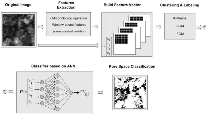
Fig. 1.The block diagram of our proposed method.
important for the measurement of properties as well as for detecting and recognising objects in the soil.
Different methods have been used to segment soil images such as a simple binary threshold method (Perret et al., 2003) and a multiple threshold method (Pal and Pal, 1993; Vogel and Kretzschmar, 1996; Capowiez et al., 1998; Tarquis et al., 2009). Vogel and Kretzschmar (1996) suggested using thresholds for typical and critical regions. They calculated a lower limit of the critical region for each individual im-age as the averim-age of the lower maximum and minimum be-tween the two maxima in the grey-level histogram. Capowiez et al. (1998) used a simple rule to determine the threshold value based on the grey-level histogram. By adding 1/3 of the distance between the pore peak and the matrix peak to the pore peak, they identified the approximate minimum of the distribution function between the two peaks. Pal and Pal (1993) suggested local thresholding schemes in which the voxel classification depends on the grey-scale values of its surrounding voxels instead of using global-level values as thresholds. Oh and Lindquist (1999) developed a local threshold method based on the Mardia-Hainsworth spatial thresholding algorithm; details on this method can be found in Mardia and Hainsworth (1988).
The aim of the present work is to detect pore space in 2-D images (that is, axial views) acquired using tomography tech-niques. The methodology is composed of three steps. The first step is called feature extraction; we applied an erosion morphological operation to enhance the dark regions (pore space). In the next step, three clustering methods were
imple-mented to segment soil images, including (K-means, Fuzzy C-means and Self Organising Maps). In the last step, an Ar-tificial Neural Network was implemented to classify soil and pore space using the segmented images. Figure 1 shows the block diagram of our proposed method. Our goal is to obtain an image in which pore and soil spaces can be distinguished.
2 Materials and methods
2.1 Soil image
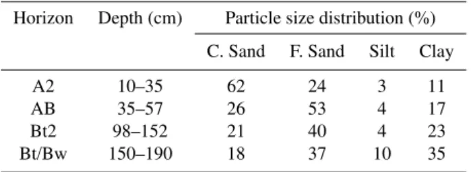
Soil samples were collected from four horizons of an argis-sol formed on the Tertiary Barreiras group of formations in Pernambuco, Brazil, at the Itapirema Experimental Station. According to the classification scheme of K¨oppen, the area has a tropical monsoon climate. The physical and chemi-cal characterisation, macromorphology and micromorphol-ogy of this soil have been broadly analysed by Melo and dos Santos (1996). The physical characteristics of the soil are provided in Table 1.
The intact soil samples were imaged using an EVS MS-MicroCT scanner (now GE Medical, London, Canada). Though some samples required paring to fit into the 64-mm-diameter imaging tubes, the field orientation was maintained. Imaging parameters were 155 keV and 25 µA.
Table 1. Physical properties of the selected horizons of Argissol according to Melo and dos Santos (1996).
Horizon Depth (cm) Particle size distribution (%) C. Sand F. Sand Silt Clay
A2 10–35 62 24 3 11
AB 35–57 26 53 4 17
Bt2 98–152 21 40 4 23
Bt/Bw 150–190 18 37 10 35
sub-volumes were extracted from each of the four original volumes using GE Medical Microview; care was taken to en-sure no overlay of the sub-volumes. The sub-volumes mea-sured 256×256×256 units, corresponding to about 16.8 mil-lion voxels. A 3-D Gaussian filter was also run in Microview (GE Healthcare, 2006) on each sub-volume to reduce noise and beam-hardening artefacts, typically occurs in CT imag-ing (Tarquis et al., 2009). In this work, we used 2-D images, these images were extracted from 3-D images.
2.2 Feature extraction
Feature extraction is the process of locating information of interest to detect pore space in soil images. The idea is that feature extraction identifies different features of the same pattern corresponding to different levels of importance and thereby carrying different information. First, an erosion mor-phological operation was applied to enhance pore areas. Sec-ond, spatial domain features were used to obtain information on the neighbourhood of each pixel; in this work, we com-puted two window-based features (namely, mean and stan-dard deviation) with different window sizes (3×3, 5×5) in the eroded image. In order to select the best size window, we calculated the correlation between the mean and standard deviation for each image.
Using the extracted features and the grey-level inten-sity of the original image, a Feature Vector (FV) was con-structed. This FV is used for image segmentation. The FV is composed asx1(qs)= {[x1(qs),x2(qs),x3(qs),x4(qs)]}, where qs=1,...,Qs. Note thatQs;=M×N, whereM×N is the
image size. x1(qs) corresponds to the grey-level intensity of the original images. x2(qs) corresponds to the grey level of the eroded image, andx3(qs)andx4(qs)correspond to the mean and standard deviation of the eroded image, respectively. 2.2.1 Mathematical morphology
Mathematical Morphology is a discipline in the field of im-age processing that involves an analysis of the structure of images. Image processing using morphological transforma-tion is a process of informatransforma-tion removal based on size and shape. In this process, irrelevant image content is
elimi-nated selectively, and thus the essential image features can be enhanced. Using the concept of structuring elements, in-tersections and unions in the image with the translations of the structuring element yield two basic morphological oper-ations, namely, erosion and dilation (Gonzalez and Woods, 2002).
Erosion generally decreases the size of objects and re-moves small anomalies by subtracting objects with radii smaller than the given structuring element. With grey-scale images, erosion reduces the brightness (and therefore the size) of bright objects on a dark background using the neigh-bourhood minimum when shifting the structuring element over the image. Erosion is denoted by
(I 2E)(x,y)=max[I (x−i,y−j )−E(i,j )], (1) whereI (x,y)is a grey-scale image, andE(i,j )is the struc-turing element.
In contrast to erosion, dilation generally increases the sizes of objects, fills in holes and broken areas and connects areas that are separated by spaces smaller than the size of the struc-turing element. With grey-scale images, dilation increases the brightness of objects by taking the neighbourhood max-imum when shifting the structuring element over the image. Dilation is denoted by
(I⊕E)(x,y)=min[I (x−i,y−j )+E(i,j )] (2) whereI (x,y)is a grey-scale image, andE(i,j )is the struc-turing element.
2.2.2 Spatial domain features
Spatial domain features include both shape-related features and window-based features. In this work, we applied window-based features. These features are the mean and standard deviation, which are extracted from images within a rectangular window.
Iµ=
1 n×m
n
X
i=1 m
X
j=1
I (i,j ) (3)
ISTD=
1 n×m
n
X
i=1 m
X
j=1
(I (i,j )−Iµ)2
!1/2
, (4)
whereIµ andISTD represent the mean and standard
devi-ation, respectively, of an image, withn×mis the window size,Iis an image and(i,j )is the pixel position.
2.3 Image segmentation using clustering techniques
2002). The segmentation of soil images is very important for the measurement of properties as well as for detecting and recognising objects in the soil. The approaches to segmenta-tion proposed in the literature vary depending on the specific application, such as CT or MRI. The main problem in CT soil images is the low contrast between soil and pore space. Pore space is represented in CT images by dark pixels (0 – grey level), and soil is represented by clear pixels (255 – grey level) (Vogel and Kretzschmar, 1996).
Tarquis et al. (2009) and Pi˜nuela et al. (2009), used the Peak Fitting Module to analyze the histogram, in order to identification of constituent peaks in the grey-scale his-togram. The major peak with the lowest mean digital num-ber was taken to be that corresponding to the pore space; the next major peak was considered to be solid soil, assuming Gaussian distribution for both peaks. In this work, we used clustering techniques based on partitional clustering. Parti-tional techniques have advantages in applications involving large data sets, for example, soil image data. Soil images present different regions in which the pore and solid mix may hinder the identification of each region. A problem that ac-companies the use of a partitional algorithm is the need to choose the number of desired output clusters. We propose and compare three clustering methods to segment soil im-ages (K-Means, Fuzzy c-Means and Self Organising Maps). These clustering methods have been used to segment natural images (Jian and Zhou, 2004; L´azaro et al., 2006; Ye, 2009), satellite images (Chuang et al., 2006; Arias et al., 2009) and mammograms images (Vega-Corona et al., 2003; De Oliveira et al., 2009; Quintanilla-Dominguez et al., 2009).
The objective of the clustering process used to segment images is to find pixel groups with a similar grey-level in-tensity in order to integrate them into homogeneous groups. Similarity is evaluated according to a distance measure be-tween the pixel and the prototypes of the object or region prototypes, and each pixel is assigned to the nearest or most similar prototype. However, this process must distribute all data to the different groups, even if some pixels are not very representative of the group as a whole (Ojeda-Maga˜na et al., 2009).
2.3.1 K-means algorithm
The K-means algorithm (MacQueen, 1967) is one of the sim-plest unsupervised learning algorithms that is used to solve the well-known clustering problem. The procedure involves a simple and easy way to classify a given data set into a cer-tain number of clusters (namely,kclusters), which is fixed a priori. The main idea is to definekcentroids, that is, one for each cluster. The next step is to take each point belonging to a given data set and associate it with the nearest centroid. When no additional points are available for clustering, the first step is completed, and an early group is done. At this point, we must re-calculateknew centroids at vary centres of the clusters resulting from the previous step. After we obtain
theseknew centroids, a new binding is conducted between the same data set points and the nearest new centroid. A loop is then generated. Based on this loop, we may notice that the kcentroids change their location step by step until no more changes occur, that is, centroids do not move anymore. Fi-nally, this algorithm minimises an objective function, which in this case is a squared error function, as follows:
J=
k
X
j=1 n
X
i=1
x
(j ) i −cj
2 , (5) where x (j ) j −ci
2
is the Euclidean distance measure be-tween a data pointx(j )j and the clustercj, which serves as an
indicator of the distance between thendata points and their cluster centres. The algorithm is composed of the following steps:
– Placekpoints into the space represented by the objects that are being clustered. These points represent the ini-tial centroids.
– Assign each object to the group with the closest cen-troid.
– When all objects have been assigned, recalculate the po-sitions of thekcentroids.
– Repeat the second and third steps until the centroids no longer move. This produces a separation of the objects into groups from which the metric to be minimised can be calculated.
Although it can be proven that the procedure will always ter-minate, the K-means algorithm does not necessarily iden-tify the most optimal configuration in terms of the global objective function minimum. The algorithm is also signifi-cantly sensitive to the initial randomly selected cluster cen-tres. However, the K-means algorithm can be run multiple times to reduce this effect.
2.3.2 Fuzzy c-means algorithm
The Fuzzy c-Means clustering algorithm (FCM) was ini-tially development by Dunn (1973) and later generalised by Bezdek (1981). This algorithm is based on optimising the objective function given by Eq. (6)
Jfcm(Z;U;V)= c
X
i=1 N
X
k=1
(µik)mkzk−vik2, (6)
where the matrixU= [µik] ∈Mfmcis a fuzzy partition ofZ,
andV= [v1,v2,...vc]is the vector of prototypes of the clus-ters, which are calculated according toDikAi= kzk−vik
2,
which is a square inner-product distance norm. m∈ [1,∞]
Fuzzy c-Means algorithm is reached by implementing the couple(U∗,V∗)to locally minimise the objective function Jfmcaccording to an alternating optimisation method
(Ojeda-Maga˜na et al., 2009).
Theorem FMC: ifDikAi= kzk−vik>0 for everyi,k,m >
1 and Z containing at least c different patterns, (U,V)∈ Mfmc× ℜc×NandJfmccan be minimised only if
µik= c
X
j=1
D
ikAi
Dj kA
i
2/(m−1)!−1
1≤i≤c; 1≤k≤n (7)
vi= N
P
k=1
µmikzk
µm ik
P
k=1
1≤i≤c (8)
Following the Eqs. (7) and (8) presented above with respect to the FCM algorithm, givenZ, choose the number of clus-ters 1≤i≤N, the weighting exponentm >1 and, the ending toleranceδ >0. Then, the solution can be reached with the following steps:
– Provide an initial value to each one of the prototypesvi,
i=1,...,c. These values are generally generated ran-domly.
– Calculate the distance of patternszk from each of the
i-th prototypesvi usingD2ikAi=(zk−vi)TAi(zk−vi),
1≤i≤c, 1≤k≤N.
– Determine the membership degrees of the matrixU= [µik], ifDikA>0 using Eq. (6).
– Calculate the new values of the prototypes vi using
Eq. (7).
– Verify if the error is greater thanδ. If it is, move on to the second step. Otherwise, stop.
2.3.3 Self Organising Maps
An artificial Neural Network (ANN) is a mathematical model that attempts to simulate the structural and functional aspects of biological neural networks. ANN can be classified as both supervised and unsupervised. The most important fea-tures that relate to an ANN with respect to biological neural networks are that knowledge is acquired through a learning process, and synaptic weights are used to store knowledge (Haykin, 1999). ANNs are considered very powerful classi-fiers compared to classical algorithms. The algorithms used in ANN applications are capable of finding good classifiers based on a limited and generally small number of training examples. This capability, also referred to as generalisation, is useful from a pattern recognition standpoint since a large set of parameters is estimated using a relatively small data set.
Self Organising Maps (SOM; Kohonen, 1990) are a type of unsupervised learning tool used for the goal of discov-ering the underlying structure of data. A topological map is simply a mapping that preserves neighbourhood relations, and it consists of a set of units that are arranged in a certain topology. SOM basically provide a form of cluster analysis by producing a mapping of high-dimensional input dataX, X∈ ℜn, in the output space while preserving the topological relationship between the input data items as faithfully as pos-sible. Each of the unitsiis assigned a weight vectormi of the same dimension as the input data, wheremi∈ ℜn. In the initial setup of the model prior to training, the weight vec-tor is filled with random values. During the learning step, the unitcwith the highest activity level, which is the win-nercwith respect to a randomly selected input patternx, is adapted in a way that will allow it to exhibit an even higher activity level at future presentations of that specific input pat-tern. Commonly, the activity level of a unit is based on the Euclidian distance between the input pattern and the pattern weight unit of that vector. The unit showing the lowest Eu-clidean distance between its weight vector and the current input vector is selected as the winner. Hence, the selection or winnercmay be written as follows:
c: kx−mck =min i kx−
mik (9) Adaptation takes place at each learning iteration and is per-formed as a gradual reduction of the difference between the respective components of the input vector and the weight vector. The amount of adaptation is guided by the learning rateα, which gradually decreases over time. As an extension to standard competitive learning, units in a time-varying and gradually decreasing neighbourhood surrounding the winner are adapted. This strategy enables the formation of large clusters in the beginning and fine-grained input discrimina-tion toward the end of the learning process. In combining these principles of SOM training, we may write the learning rule as given in Eq. (10):
mi(t+1)=mi(t )+α(t )hci[x(t )−mi(t )], (10) wheret denotes the current learning iteration, andα repre-sents the time-varying learning rate. ci represents the
time-varying neighbourhood kernel, andx represents the current input pattern. Finally,mi denotes the weight vector assigned to uniti.
2.4 Classification
An ANN was used to classify soil images into two classes (pore space and solid soil). ANN is characterised by a great degree of modularity and flexibility, also it is very efficient for demanding large-scale and generic pattern recognition applications.
2.4.1 Feed Forward Neural Network
Feed Forward Neural Network (FFNN), also known as mul-tilayer perceptrons (MLP), are popularly used in many prac-tical applications. FFNN is a type of supervised learning. Knowledge is acquired by the network through a learning process known as the Back Propagation (BP) algorithm. The BP algorithm serves as a workhorse in the design of a spe-cial class of layered FFNN. A FFNN has an input layer of source nodes and an output layer of neurons; these two lay-ers connect the network to the outside world. In addition to these two layers, the multilayer perceptron usually has one or more layers of hidden neurons, which are called hidden because they are not directly accessible. The hidden neurons extract important features contained in the input data. Using supervised learning, these networks can learn the mapping from one data space to other examples. The term BP refers to the way in which the error is computed at the output side. Namely, it is propagated backwards from the output layer to the hidden layer and finally to the output layer; details on this method can be found in Basheer and Hajmeer (2000).
Three FFNN with the same structure were tested, one for each segmentation method. The network structures used are as follows:
– Input layer: four neurons, where each neuron is an image feature.
– Hidden layer: one hidden layer with ten neurons. – Output layer: one output layer, where in the output layer
two classes are obtained. – Learning rate: 1.
– The used activation function: the log-sigmoid function. – Training set: eight images, two for each horizon. – Training conditions: epoch=250.
– Performance function: Mean Squared Error (MSE)=0.01.
– Test set: four images, an image for each horizon. All mathematical computations were performed using Matlab®.
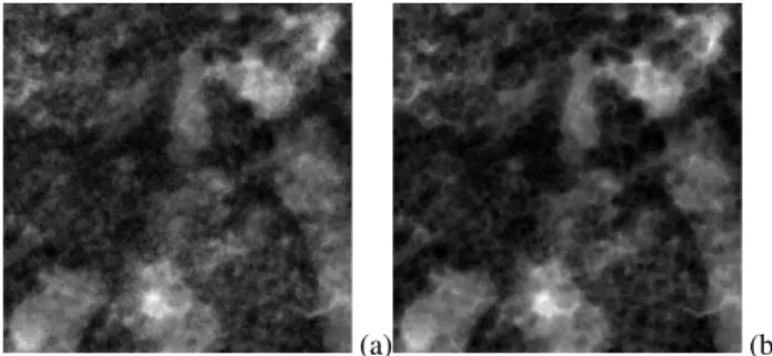
(a) (b)
Fig. 2.The obtained result for a soil image: (a) the CT soil image in grey scale; (b) the results after a morphological erosion operation.
3 Results and discussion
3.1 Feature extraction
For each studied image, we applied an erosion morphological operation to enhance the dark regions (that is, pore space). The structuring element will darken the image. Bright re-gions surrounded by dark rere-gions (pore space) shrink in size, and dark regions surrounded by bright regions (that is, soil solid) grow in size. Small, bright pixels in images will dis-appear as they are eroded down to the surrounding intensity value, and small dark pixels will become larger pixels. The effect is most marked at places in the image where intensity changes rapidly, whereas regions with fairly uniform inten-sity will be left more or less unchanged, except at their edges. A cross-shaped structuring element of 3×3 size window was applied. Figure 2 shows the results for a given image. Fig-ure 2a shows grey-scale CT soil images. FigFig-ure 2b depicts the results after a morphological erosion operation.
In this work, we applied two window-based features, namely, mean and standard deviation; they were extracted from eroded images within a rectangular window. Two win-dows of different sizes were applied. The correlation analysis was implemented to find the best pixel block window accord-ing to the results already obtained; as such, we chose a 5×5 pixel window.
3.2 Image segmentation
Three clustering methods were implemented to obtain seg-mented images. We built a FV,Ss= {x(qs):qs=1,...,Qs},
where x(qs)∈ ℜD is a D-dimensional vector, and Qs
is the number of pixels in the image, where x(qs) = {[x1(qs),x2(qs),x3(qs),x4(qs)]}. The FV set is then clustered us-ing three different methods.
Ss are grouped intokclusters, where only one group
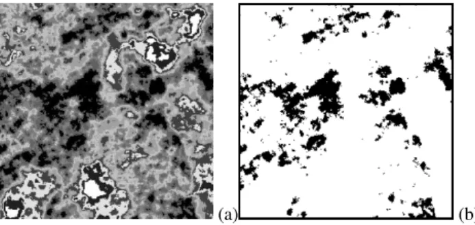
(a) (b)
Fig. 3.The obtained results for the K-means method:(a)the image segmented with nine clusters; and(b)the binary image obtained from the segmentation process, where 0 value corresponds to the pore space class and 1 value corresponds to the soil solid class.
segmented image of binary form, where 0 value corresponds to a pore space class and 1 value corresponds to a soil solid class. Next, we show the initial conditions for segmentation and the results of each clustering method.
In the implementation of segmentation algorithm is nec-essary to have information about the images, this informa-tion help us to adjust the parameters and number of groups in which the image will be segmented. Once we know how many groups are needed to represent the gray levels corre-sponding to pore, more images with the same features can be segmented.
3.2.1 K-means
The initial conditions for this method were as follows. – The cluster number took values from 7 to 11. – Centroids were initialised as random values.
– The Euclidean distance function was used to measure distance.
– The maximum iteration number was set at 100. To illustrate the results, Fig. 3 shows the segmented image and the binary image obtained by applying the K-means al-gorithm.
3.2.2 FCM
The initial conditions for this method were as follows: – The cluster number took values from 7 to 11. – Centroids were initialised as random values. – The number of membership degrees was set to 2. – The maximum number of iterations was set to 100. – The minimum amount of improvement was set to
1×10⁻³.
To illustrate the results, Fig. 4 shows the segmented and binary images obtained by applying FCM algorithm.
(a) (b)
Fig. 4.The obtained results for the Fuzzy c-means method:(a)the image segmented with nine clusters; and(b)the binary image ob-tained from the segmentation process, where 0 value corresponds to the pore space class and 1 value corresponds to the soil solid class.
(a) (b)
Fig. 5. The obtained results for the SOM method: (a)the image segmented with nine clusters; and(b)the binary image obtained from the segmentation process, where 0 value corresponds to the pore space class and 1 value corresponds to the soil solid class.
3.2.3 SOM
The initial conditions for this method were as follows: – The network structure [4k] was such thatktook values
from 7 to 11.
– The weight vector was randomly initialised. – The topology function was hextop.
– The distance function was linkdist. – The maximum epoch was set at 100.
To illustrate these results, Fig. 5 shows the segmented and binary images obtained by applying SOM.
The group corresponding to the pore class was obtained under the following conditions.
Table 2.Porosity percentages using thresholding criteria (Pi˜nuela, 2009).
Horizon Porosity (%)
A2 13.45
AB 14.73
Bt2 12.14
Bt/Bw 12.76
equal to 9. Care must be taken not to over-segment the age, therefore it is necessary to have information of the im-age when the algorithm is implemented. Table 2 shows the porosity percentage from Pi˜nuela et al. (2009). Table 3 shows the percentage of pore space obtained using our method, the results show that the more the image is segmented group that corresponds to the pore is divided, for this reason the per-centage of pore decreases. Based on this comparison, the FV was clustered and labelled into nine groups. These labelled vectors were then used for classification.
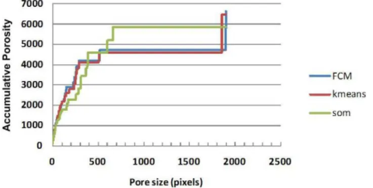
3.2.4 Pore space distribution
In this study, we observed that it is not only the percentage of porosity that influences the threshold method; in addition, certain pore sizes present a higher influence, as is shown in Fig. 6. Pores with sizes ranging from 50 pixels to 400 FCM and K-means show a similar accumulative porosity curve; meanwhile, SOM shows a lower increase. For pores that are greater than 400 pixels, the accumulative curves decrease until the pore size reaches 2000 pixels under the FCM and -means algorithms. However, in terms of total porosity, this may not be significant, especially considering the substantial influence of hydraulic simulation and behaviour.
3.3 Image classification
We used 2-D CT soil images to detect the percentage of pore space in soil. The image resolution is 45.1 µm, and the image size is 256×256 pixels, so that we have 65 536-pixels by im-age. We built a FV from the setSs, which includes 786 432
feature vectors obtained from feature extraction (pixels cor-responding to twelve images). Then, we clustered and la-belled FV into the setSsusing the K-means, FCM and SOM
algorithms to compare results. Each FV was partitioned into two sets, namely, a training set with 524 288 feature vectors and a test set with 262 144 feature vectors.
The classification results are represented by the output vector (Vout). Three FFNNs were used for training and test-ing with the same conditions to compare classification re-sults.
Classification was performed for each FV obtained in the clustering step. Table 4 shows the results of the classification for each FV (test set). The output of FFNNs were compared
Fig. 6.Pore space distribution for the A2 horizon.
with FV label. According to the obtained results, the best classification rate was obtained using the FV for the K-means algorithm.
3.3.1 Image reconstruction
Voutcontains the classification results, whereVoutis formed by two classes, with one corresponding to solid soil and the other corresponding to pore space. UsingVout, we built four images and computed the pore percentage for each recon-structed image. These results are compared with the obtained percentage in Table 3.
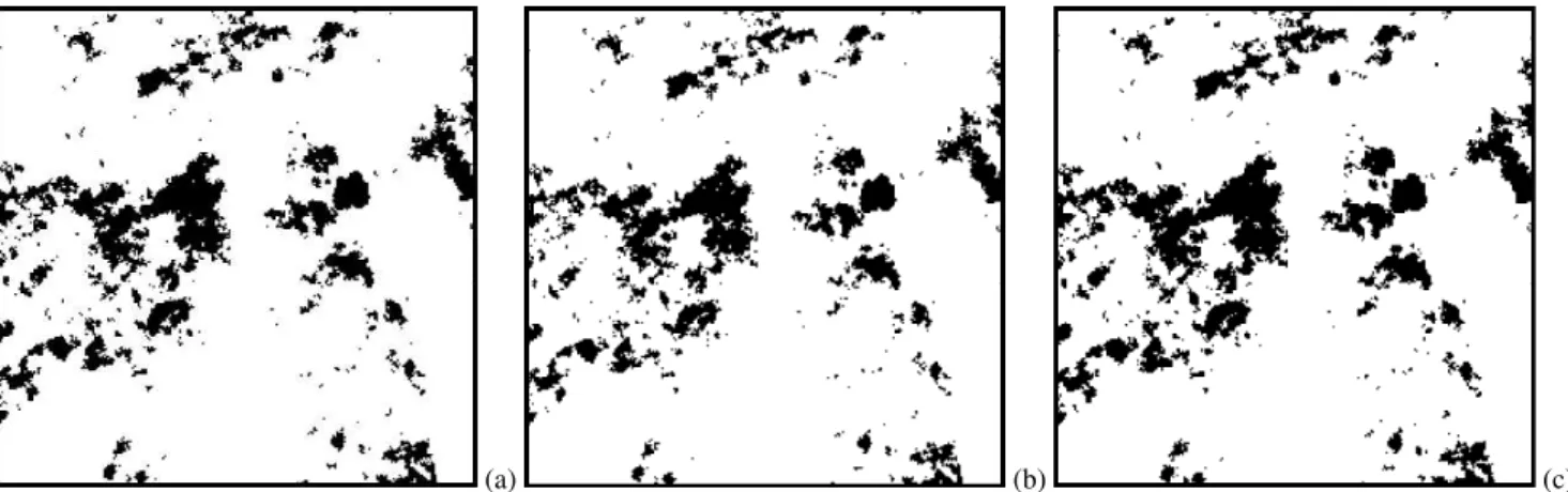
Table 5 shows the comparison results, where the initial percentage obtained in the segmented images is compared with the classifier output. In the results, we can observe that the final percentages obtained for A2, Bt2 and Bt/Bw hori-zons are very similar to initial percentage, but with the AB horizon, the classifier has a very big mistake. The method has limitations in the classification of the AB horizon, to im-prove the outcome in future work will analyze the feature extraction and segmentation in order to improve the classi-fication. Figure 7 shows the reconstructed image for each Vout, the obtained classification is represented as binary im-age where 0 value corresponds to the pore space class and 1 value corresponds to the soil solid class.
4 Conclusions
This paper proposed an alternative way to detect pore space in CT soil images using image processing, data clustering and ANN. Feature extraction in soil images is an important factor for the pore space detection due to the low level of con-trast in these image types. We applied an erosion morpho-logical operation to enhance the dark regions (pore space); in addition, the mean and standard deviation were used to generate additional information about areas of interest.
(a) (b) (c)
Fig. 7.The obtained classification results, in each image 0 value (black) corresponds to the pore space class and 1 value (white) corresponds to the soil solid class: (a)the classification obtained with the K-means segmented images;(b)the classification obtained with the FCM segmented images; (c)the classification obtained with the SOM segmented images. The binary image obtained from the segmentation process.
Table 3.The percentage of pore space obtained in clustering methods for each horizon, where the cluster number takes values ranging from 7 to 11.
No. of Clusters K-Means (%) Fuzzy C-Means (%) SOM (%)
A2 AB Bt2 Bt/Bw A2 AB Bt2 Bt/Bw A2 AB Bt2 Bt/Bw
7 19.60 18.00 14.13 16.94 18.11 16.80 13.86 15.96 20.44 18.52 17.46 18.66 8 16.72 15.17 13.35 13.42 15.54 13.79 11.87 13.34 17.79 15.89 14.77 16.02 9 13.57 11.86 11.98 12.06 13.32 11.70 10.46 11.61 15.59 13.83 12.77 13.95 10 11.92 10.15 10.11 11.98 11.49 10.00 0.27 10.51 13.80 12.11 11.27 12.47
11 9.58 8.84 6.25 10.39 10.00 8.79 8.36 9.16 12.45 10.74 10.04 11.13
Table 4.The classification percentages obtained for each FV.
FV for Correct classification clustering method (%)
K-means 97.01
FCM 96.44
SOM 96.12
Table 5.Porosity percentages for FFNN classifications.
Horizon K-Means (% ) Fuzzy C-Means (%) SOM (%)
Initial Final Initial Final Initial Final
percentage percentage percentage percentage percentage percentage
A2 13.57 13.30 13.32 12.29 15.59 14.83
AB 11.86 3.45 11.70 3.03 13.83 3.98
Bt2 11.98 14.55 10.46 13.06 12.77 16.68
provide a set of centroids as the most representative elements of each group. As such, clustering algorithms partition the input images in homogeneous areas, each of which is con-sidered homogeneous with respect to a property of interest.
Unlike image segmentation based on histograms, this method allows a deeper analysis of the areas where the pore and soil are mixed because segmentation by clustering facili-tates the analysis of multidimensional data, while segmenta-tion using histogram analysis allows us to analyse only one dimension.
In this work, we proposed an ANN as a classifier. ANN has been used with success in different investigation fields. This classifier plays an important role in our methodology because ANN can learn structure in data through examples contained in a training set and then can conduct complex de-cision making. Our methodology provides an alternative way to detect solid soil and pore space in CT images. The percent-ages of correct classifications of pore space in impercent-ages were 97.01%, 96.47 % and 96.12%.
Acknowledgements. The authors wish to thank the National
Council for Science and Technology (CONACyT), the Secretariat of Public Education (SEP), the Government of Mexico and the Group of Automation in Signals and Communications (GASC) of the Technical University of Madrid. Funding provided by Spanish Ministerio de Ciencia e Innovaci´on (MICINN) through project no. AGL2010-21501/AGR is greatly appreciated.
Edited by: Q. Cheng
References
Arias, S., G´omez, H., Prieto, F., Bot´on, M., and Ramos, R.: Satellite image classification by self organized maps on GRID computing infrastructures, Proceedings of the second EELA-2 Conference, 1–11, 2009.
Basheer, I. A. and Hajmeer, M.: Artificial neural networks fun-damentals, computing, design, and application, J. Microbiol. Meth., 43, 3–31, 2000.
Bezdek, J. C.: Pattern Recognition with Fuzzy Objective Function Algorithms, Plenum Press, New York, 1981.
Capowiez, Y., Pierret, A., Daniel, O., Monestiez, P., and Kret-zschmar, A.: 3D skeleton reconstructions of natural earthworm burrow systems using CAT scan images of soil cores, Biol. Fert. Soils, 27, 51–59, 1998.
Chuang, K. S., Tzeng, H. L., Chen, S., Wu, J., and Che, T. J.: Fuzzy c-means clustering with spatial information for image segmenta-tion, Comput. Med. Imag. Grap., 30, 9–15, 2006.
De Oliveira, L., Braz, G., Correa, A., Cardoso, A., and Gattas, M.: Detection of masses in digital mammograms using K-means and support vector machine, Electronic letters on computer vision and images analysis, 8(2), 39–50, 2009
Dunn, J. C.: A Fuzzy relative of isodata process and its use in de-tecting compact well-separated clusters, J. Cybernetics, 3, 32– 57, 1973.
GE Healthcare: Microview 2.1.2 – MicroCT Visualization and Analysis, London, Canada, 2006.
Gonzalez, R. C. and Woods, R. E.: Digital image processing, Pren-tice Hall, New Jersey, 2002.
Haykin, S.: Neural Networks: A comprehensive foundation, Pren-tice Hall, New Jersey, 1999.
Jian, Y. and Zhou, Z. H.: SOM Ensamble-based image segmenta-tion, Neural Process. Lett., 20, 171–178, 2004.
Kohonen, T.: The self organizing map (SOM), Proceedings of the IEEE, 78(9), 1464–1480, 1990.
L´azaro, J., Arias, J., Mart´ın, J. L., Zoloaga, A., and Cuadrado, C.: SOM segmentation of gray scale images for optical recognition, Pattern Recogn. Lett., 27, 1991–1997, 2006.
MacQueen, J. B.: Some Methods for classification and Analysis of Multivariate Observations, Proceedings of 5-th Berkeley Sympo-sium on Mathematical Statistics and Probability, Berkeley, Uni-versity of California Press, 1, 281–297, 1967.
Mardia, K. V. and Hainsworth, T. J.: A Spatial Thresholding Method for Image Segmentation, IEEE T. Pattern Anal., 10(6), 919–927, 1988.
Melo, F. J. R. and dos Santos, M. C.: Micromorfologia e minera-log´ıa de dois solos de Tabuleiro costeiro de Pernambuco, R. Bras. Ci. Solo, 20, 99–108, 1996.
Mermut, A. R.: Historical Development in soil micromorphological imaging, J. Mt. Sci., 6, 107–112, 2009.
Oh, W. and Lindquist, B.: Image thresholding by indicator kriging, IEEE T. Pattern Anal., 21, 590–602, 1999.
Ojeda-Maga˜na, B., Quintanilla-Dominguez, J., Ruelas, R., and An-dina, D.: Images sub-segmentation with the PFCM clustering al-gorithm INDIN 2009, 7th IEEE International Conference, 499– 503, 2009.
Pal, N. R. and Pal, S. K.: A review of image segmentation tech-niques, Patt. Recogn., 29, 1277–1294, 1993.
Perret, J. S., Prasher, S. O., and Kacimov, A. R.: Mass fractal di-mension of soils macropores using computed tomography: from the box counting to the cube-counting algorithm, J. Hydrol., 267, 285–297, 2003.
Pi˜nuela, J., Alvarez, A., Andina, D., and Tarquis, A. M.: Quantify a soil pore distribution from 3D images: Multifractal sprectrum through wavelet approach, Geoderma, 155, 203–210, 2009. Quintanilla-Dominguez, J., Cortina-Januchs, M. G.,
Barr´on-Adame, J. M., Vega-Corona, A., Buend´ıa-Buend´ıa, F. S., and An-dina, D.: Detection of microcalcification using coordinate logic filters and artificial neural networks, Lect. Notes Comput. Sc., 5602, 179–187, 2009.
Tarquis, A. M., Heck R. J., Andina, A., and Ant´on, J. M.: Pore network complexity and thresholding of 3D soil images, Ecol. Complex., 6, 230–239, 2009.
Vega-Corona, A., ´Alvarez-Vellisco, A., and Andina, D.: Feature vectors generation for detection of microcalcification in digitized mammography using neural network, Lect. Notes Comput. Sc., 2687, 583–590, 2003.
Vogel, H. J. and Kretzschmar, A.: Topological characterization of pore space in soil-sample preparation and digital image-processing, Geoderma, 73, 23–38, 1996.