Luiz Carlos Pessoa Albini
Unicenp, Dept. Informatics R. Prof. Pedro Viriato Parigot de Souza, 5300
81280-330, Curitiba, PR Brazil [email protected]
Elias Procópio Duarte Jr.
Roverli Pereira Ziwich
Federal University of Paraná, Dept. Informatics P.O.Box 19081 – Curitiba
81531-990, PR Brazil {elias,roverli}@inf.ufpr.br
Comparison-Based
System-Level Diagnosis
Abstract
This work introduces a new system-level diagnosis model and an algorithm based on this model: Hi-Comp (Hierarchical Comparison-based Adaptive Distributed System-Level Diagnosis algorithm). This algorithm allows the diagnosis of systems that can be represented by a com-plete graph. Hi-Comp is the first diagnosis algorithm that is, at the same time, hierarchical, distributed and com-parison-based. The algorithm is not limited to crash fault diagnosis, because its tests are based on comparisons. To perform a test, a processor sends a task to two processors of the system that, after executing the task, send their puts back to the tester. The tester compares the two out-puts; if the comparison produces a match, the tester con-siders the tested processors fault-free; on the other hand, if the comparison produces a mismatch, the tester considers that at least one of the two tested processors is faulty, but can not determine which one. Considering a system of N nodes, it is proved that the algorithm’s diagnosability is (N–1) and the latency is log2N testing rounds. Further-more, a formal proof of the maximum number of tests re-quired per testing round is presented, which can be O(N3).
Simulation results are also presented.
Keywords:Distributed Diagnosis, System-Level Di-agnosis, Comparison-Based Diagnosis.
1. INTRODUCTION
The basic goal of system-level diagnosis is to determine the state of all units of a given system [1]. Each unit may be either faulty or fault-free. Fault-free units perform tests over other units to achieve the complete diagnosis.
System-level diagnosis has been applied to different fields, such as network fault management and circuit fault detection. The model and algorithm presented in this paper can be employed to detect changes in servers that keep replicated data, such as Web or file servers.
A number of different system-level diagnosis models [2] have been presented in the literature. The first system-level diagnosis model, the PMC model, was introduced in [3]. In the PMC model, system diagnosis hinges on the ability of units to test the status of other units. A unit can be either faulty or fault-free and its state does not change during diagnosis. Each change on the state of a node is called an event. In this model, a test involves controlled application of stimuli and observation of the corresponding responses. The set of all test outcomes is called the syndrome. The model assumes that fault-free units always report the state of the units they test correctly, while faulty units can return incorrect results [4, 1, 3]. The minimum number of units that must be fault-free for diagnosis to be possible is called the diagnosability.
Many algorithms based on the PMC model have been proposed. In the adaptive algorithms nodes decide the next tests based on results from previous tests [5], the
distributed algorithms allow the fault-free nodes in the system to diagnose the state of all nodes [6], and in [7] a
hierarchical algorithm is presented.
with Timestamps performs event diagnosis. This algorithm groups the units of the systems into sets of N/2 units called clusters. When a tester tests a fault-free unit it gets diagnostic information about the tested unit entire cluster. Each unit of a system running Hi-ADSD with Timestamps keeps a timestamp for the state of each other unit in the system, so a tester may get diagnostic information about a certain unit from more than one tested unit without causing any inconsistencies.
The way tests are performed in the PMC model suffers from several limitations that have caused other testing methods to be considered, like probabilistic diagnosis [11] and the comparison-based models presented below.
The comparison-based models, proposed initially by Malek [12], and by Chwa and Hakimi [13], have been considered to be a practical approach for fault diagnosis in distributed systems. In these first comparison-based models, it was assumed that system tasks are duplicated on two distinct units in the system and their outputs are compared by a central observer. This central observer is a reliable unit that cannot suffer any event. The observer performs diagnosis using the comparisons’ outcomes.
Maeng and Malek present an extension of the Malek’s comparison-based model, known as the MM model [14]. This model allows comparisons to be carried out by the units themselves, i.e., the comparisons are distributed. The unit that performs the comparison must be distinct from the two units that produce the outputs. Sengupta and Dahbura present a generalization of the MM model in [15], known as the generalized comparison model, which allows the tester unit to be one of the units which produce the outputs. In both the MM model and the generalized comparison model, although the comparisons are distributed, the comparisons’ outcomes are still sent to a central observer, and only the central observer performs the diagnosis.
In [16], Blough and Brown present a distributed diagnosis model based on the comparison approach, the so-called Broadcast Comparison model. In this model, a distributed diagnosis procedure is used, which is based on comparisons of redundant task outputs and has access to a reliable broadcast protocol. In the Broadcast Comparison model, tasks are assigned to pairs of distinct units. These units execute the task and send their outputs to all fault-free units in the system employing a reliable broadcast protocol. Each fault-free unit in the system receives and compares the two outputs eventually achieving the complete diagnosis. Note that comparisons are performed on every fault-free unit, including the processors that execute the task. The main purpose of this model is to reduce the latency and the time in which one node must remain in a given state, not the number of tests or comparisons executed.
Wang [17] presents the diagnosability of hypercubes [18, 19] and the so-called enhanced hypercubes [20], considering a comparison-based model. The enhanced hypercube is obtained by adding more links to the regular hypercube. These extra links increase the system’s diagnosability. Each processor executes tests on other processors by comparing tasks outputs. This model allows the tester to be one of the processors that have the tasks outputs compared.
Araki and Shibata [21] present the diagnosability of butterfly networks [22] using the comparison approach. Two comparison schemes for generating syndromes on butterfly networks are proposed. One is called one-way comparison, and the other is called two-way comparison. Tests involve sending the same task to two processors. Then the comparison of these two task outputs is performed by a third processor. The diagnosability of a k-ary butterfly network considering the one-way comparison scheme is k–2 and the diagnosability of the two-way scheme is 2(k–2).
Fan [23] presents the diagnosability of crossed cubes – a hypercube variant, but with lower diameter – under the comparison-based diagnosis model. The diagnosability of crossed cubes with n≥≥≥≥≥ 4 processors is n.
In this paper, we present a new distributed comparison-based model for system-level diagnosis. An algorithm based on this model is presented, the
Hierarchical Comparison-Based Adaptive Distributed System-Level Diagnosis (Hi-Comp) algorithm. This algorithm uses a similar hierarchical testing strategy as the one employed by Hi-ADSD with Timestamps. As Hi-Comp is comparison-based, it is not limited to permanent fault diagnosis, like the hierarchical distributed algorithms based on the PMC model. The diagnosability of the algorithm is presented, as well as formal proofs of the algorithm’s latency and maximum number of tests required.
The rest of work is organized as follows. In section 2 we present the new model. Section 3 introduces the new algorithm. Section 4 presents the formal proofs for the algorithm’s latency, maximum number of tests and diagnosability. In section 5 simulation results are presented and section 6 contains the conclusion.
2. THE DISTRIBUTED COMPARISON MODEL
System S is fully connected, i.e., there must exist a communication link between any pair of nodes in the system. Therefore, graph G is a complete graph, i.e., and
, .
A fault-free node tests other nodes of the system to identify their states. A test is performed by sending a task to two distinct nodes of the system. After executing the task, each node sends the task output to the tester. After receiving the two outputs, the tester compares the outputs. If the comparison produces a match the tester considers the two tested nodes as fault-free. If the comparison produces a mismatch the tester considers that at least one of the two tested nodes is faulty, but cannot conclude which one. To assure that the comparison outcomes are correct, the following assumptions are made over the system:
1. A fault-free processor comparing outputs produced by two fault-free nodes always produces a match.
2. A fault-free processor comparing outputs produced by a faulty node and any other node, faulty or fault-free, always produces a mismatch.
3. The time for a fault-free node to produce an output for a task is bounded.
To guarantee that assumption 2 is satisfied, two faulty nodes must produce different outputs for a same task.
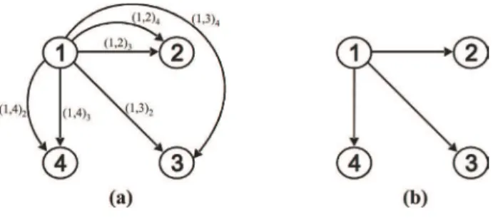
A multi-graph [24], M(S), is defined to represent the way that tests are executed in the system. M(S) is a directed multi-graph defined over graph G, when all nodes of the system are fault-free. The vertices of M(S) are the nodes of system S. Each edge in M(S) represents that a node is sending a task to another node, i.e., there is an edge from node i to node j when node i sends a task to node j. Furthermore, if node i sends a task to be executed by nodes
j and k, then there is an edge from node i to node j identified by (i,j)k and there is an edge from node i to node k identified by (i,k)j. So, if there is an edge (i,j)k from node i to node j
then there must exist an edge (i,k)j from node i to node k. As an example consider figure 1a, as node 1 sends tasks to node 2, to node 3 and to node 4, the edges are: (1,2)3, (1,3)2, (1,2)4, (1,4)2, (1,3)4 and (1,4)3, and all edges are from node 1 to the other nodes. Edge (1,2)3 indicates that node 1 sent a task to node 2 and the output of this task will be compared with the output produced for this same task by node 3, therefore the edge (1,3)2 must also be in the graph.
Figure 1. a) Multi-graph M(S). b) Graph T(S).
The model uses a graph T(S), defined over multi-graph M(S), to depict the tests executed by fault-free nodes, the Tested Fault-Free graph. In this graph, there is an edge from node i to node j when there is at least one edge from node i to node j in M(S). Figure 1b shows the graph T(S) for the multi-graph M(S) presented in figure 1a.
The diagnostic distance between node i and node j
is defined as the shortest distance between node i and node j in T(S), i.e. the shortest path between node i and node j. For example, in figure 1b the diagnostic distance between node 1 and node 3 is 1, because the shortest path between these two nodes has one edge.
3. THE HIERARCHICAL
C
OMPARISON-B
ASEDA
LGORITHMIn this section the new Hierarchical Comparison-Based Adaptive Distributed System-Level Diagnosis ( Hi-Comp) algorithm is presented. This algorithm is based on the model presented in section 2.
The algorithm employs a testing strategy represented by T(S) graph. T(S) is a hypercube when all nodes in the system are fault-free. Figure 2 shows the graph
T(S) for a system of 8 nodes.
The Tested Fault-Free graph of node i, Ti(S), is a directed graph defined over T(S) and shows how the diagnostic information flows in the system. There is an edge in Ti(S)from node a to node b if there is an edge in T(S) from node a to node b and the diagnostic distance between node
i and node a is shorter than the diagnostic distance between node i and node b. Figure 3 shows T0(S) for a system of 8 nodes. For instance, there is an edge from node 1 to node 3 in this figure, because the diagnostic distance between node 0 and node 1 is shorter than the distance between node 0 and node 3.
Nodes with diagnostic distance 1 to node i are called
sons of node i. In figure 3 the sons of node 0 are nodes 1, 2 and 4.
A testing round is defined as the interval of time that all fault-free nodes need to obtain diagnostic information about all nodes of the system. An assumption is made that after node i tests node j in a certain testing round, node j
cannot suffer an event in this testing round.
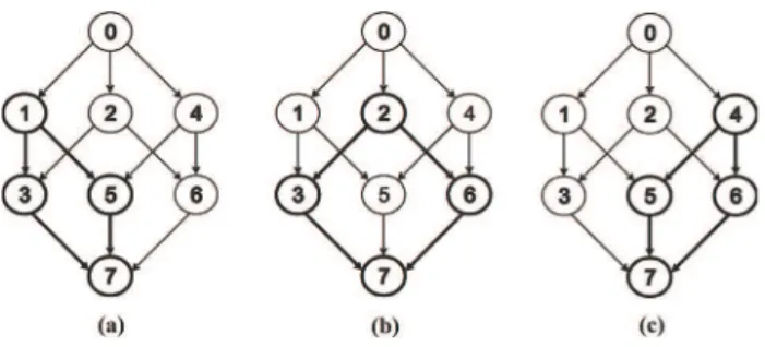
The testing strategy groups the nodes into clusters like the Hi-ADSD with Timestamps algorithm [10]. Each cluster has N/2 nodes. A function, based on the diagnostic distance, defines the list of nodes about which node i can obtain diagnostic information through a given node p. Figure 3 depicts the cluster division for a system of 8 nodes in
T0(S). The clusters are: (a) nodes {1, 3, 5, 7}, (b) nodes {2, 3, 6, 7} and (c) nodes {4, 5, 6, 7}.
Figure 3. Cluster division for a system of 8 nodes in T0(S).
3.1 Hi-Comp: Description
In Hi-Comp tests are made by sending a task to two distinct nodes that execute this task and send the outputs to the tester. This algorithm diagnoses events and states.
Initially, node i sends a task to its sons in pairs. For example, for a system of 16 nodes shown in figure 4, node 0 sends a task to nodes 1 and 2; then it sends another task to nodes 4 and 8. When the quantity of sons is odd, the last node is tested with the previous one. For example, for a system of 8 nodes shown in figure 2, node 0 sends a task to nodes 1 and 2; then it sends another task to nodes 2 and 4.
Figure 4. System with 16 nodes.
When node i diagnoses that two nodes are fault-free, by comparing the outputs produced by these nodes, node i obtains from these nodes diagnostic information about the entire clusters to which each of the tested nodes belongs.
In this algorithm it is possible that node i receives diagnostic information from node j through two or more nodes p and p’, because a node can belong to more than one cluster, as shown in figure 3. Thus, it is necessary to guarantee that node i has always the most recent diagnostic information about the other nodes. In order to allow nodes to determine the order in which events were detected, the algorithm employs timestamps [10, 25].
When node i receives diagnostic information about node j through node p, node i compares its own timestamp about node j with node p’s timestamp about node j, if the comparison indicates that node p’s information is more recent then node i updates its own diagnostic information; otherwise, node i rules the information received from node
p out.
When node i executes a comparison of outputs and this comparison indicates a mismatch, node i classifies the state of the two nodes as undefined, because it is not possible to determine which node is faulty and which is fault-free. At this point, if node i has already identified any fault-free node, it tests this fault-free node with the two undefined nodes in question, each in turn. If an output comparison indicates a match then node i classifies the tested node as free, changing from undefined to fault-free, otherwise node i classifies the tested node as faulty, changing from undefined to faulty. Meanwhile, if node i
has not yet diagnosed any fault-free node, these two nodes stay as undefined until node i diagnoses a fault-free node that could be used to diagnose the undefined ones.
If any comparison indicates a match, the tester classifies these nodes as fault-free, and the tester may then determine the state of all other nodes of the system, either by receiving diagnostic information about these nodes, or by testing the undefined nodes with the fault-free ones.
If, after testing the last node, no fault-free node was found, the tester assumes itself as fault-free and tests all nodes with itself. Now, if a comparison indicates a mismatch, the tester classifies this node as faulty; if a comparison indicates a match, the tester classifies the tested node as fault-free.
3.2 HI-COMP: SPECIFICATION
The new algorithm works over three sets: the set of undefined nodes: U, the set of faulty nodes: F and the set of fault-free nodes: FF. These sets have some properties:
Each node of the system keeps these three sets, the contents of which can vary from node to node. By the end of a testing round set U is always empty.
When node i compares the outputs of a task performed by nodes p and p’ and this comparison indicates a match, node i identifies the two tested nodes as fault-free. Node i puts the tested nodes in the set FF removing them from the set to which they belonged. When node i identifies one fault-free node, node i gets from this node diagnostic information about the whole cluster to which the fault-free node belongs. Each cluster contains N/2 nodes. Furthermore, as information is timestamped, node i must test if the received information is newer than its own information. If the received information is newer, node i
must update its own information; otherwise, node i simply rules the received information out. In other words:
send_task(p,p’);
IF (output(p) == output(p’)) THEN
U = U - {p}; U = U - {p’}; F = F - {p}; F = F - {p’};
FF = FF + {p} + {p’};
GET diagnostic information from p;
IF (diagnostic information is newer) THEN update local diagnostic information;
GET diagnostic information from p’;
IF (diagnostic information is newer) THEN update local diagnostic information;
If node i’s comparison indicates a mismatch when comparing p’s and p’’s outputs, node i classifies these nodes as undefined. Node i puts these nodes in set U removing them from the set to which they belonged. In other words:
send_task(p,p’);
IF (output(p) != output(p’)) THEN
FF = FF - {p}; FF = FF - {p’}; F = F - {p}; F = F - {p’}; U = U + {p} + {p’};
Before node i puts a node p in set U, node i must test node p with all nodes . If all these comparisons indicate mismatches node i puts node p in set U. In other words:
send_task(p,p’);
IF (output(p) != output(p’)) THEN
REPEAT for all k in U send_task(p,k);
UNTIL (k == last node in U); IF (no comparison between p and k indicates a match)
THEN
FF = FF - {p}; F = F - {p}; U = U + {p};
REPEAT for all k in U send_task(p’,k);
UNTIL (k == last node in U); IF (no comparison between p’ and k indicates a match)
THEN
FF = FF - {p’}; F = F - {p’}; U = U + {p’};
Considering the comparisons between node p and node , when one of these comparisons produces a match, the tester can classify nodes p and k as fault-free, and all the other nodes as faulty. In other words:
send_task(p,p’);
IF (output(p) != output(p’)) THEN
REPEAT for all k in U send_task(p,k);
UNTIL (output(p) == output(k)OR (k == last node in U);
IF (output(p) == output(k)) THEN
U = U - {p}; F = F - {p}; FF = FF + {p}; U = U - {k}; FF = FF + {k}; F = F + U; ELSE
FF = FF - {p}; F = F - {p}; U = U + {p};
REPEAT for all k in U send_task(p’,k);
UNTIL (output(p’) == output(k)OR k == last node in U);
IF (output(p’) == output(k)) THEN
U = U - {p’}; F = F - {p’}; FF = FF + {p’}; U = U - {k}; FF = FF + {k}; F = F + U; ELSE
FF = FF - {p’}; F = F - {p’}; U = U + {p’};
When a node is identified as fault-free by node i, node i gets the N/2 items of diagnostic information about the tested node’s cluster.
If after node i tests its sons, set U is empty and there are some nodes about which node i does not have diagnostic information, node i must test these nodes with one node previously identified as fault-free in this testing round.
If after node i tests its sons, set FF is empty, i.e. all sons of node i are classified as undefined, node i must test the sons if its sons, and so on until a comparison indicates a match, or node i tests the last node in Ti(S).
If node i tests the last node in Ti(S), node i must send tasks to this node and all nodes , one by one. In other words:
REPEAT for all k in U send_task(p,k);
UNTIL (output(p) == output(k) OR (k == last node in U);
IF (output(p) == output(k)) THEN
U = U - {p}; F = F - {p}; FF = FF + {p}; U = U - {k}; FF = FF + {k}; F = F + U; ELSE
FF = FF - {p}; F = F - {p}; U = U + {p};
If after testing all nodes in Ti(S), set FF remains empty, node i assumes itself as fault-free and tests all nodes with itself. Mismatches indicate that node k is faulty and matches indicate that node k is fault-free. In other words:
REPEAT for all k in U send_task(i,k);
UNTIL (output(i) == output(k) OR (k == last node in U);
IF (output(i) == output(k)) THEN
U = U - {k}; FF = FF + {k}; F = F + U; ELSE
U = U - {k}; F = F + {k};
Thus, by the end of a testing round, every fault-free node has set and all the nodes either in F or FF, i.e. .
The algorithm in pseudo-code is given below.
Algorithm running at node i:
TO_TEST = {ALL NODES};
U = EMPTY; F = EMPTY; FF = EMPTY;
REPEAT FOREVER
REPEAT
p = next_pair_to_test; p’ = next_pair_to_test;
IF (result == 0) /*p and p’ are tested fault-free */
THEN
U=U-{p, p’}; F=F-{p, p’}; FF=FF+{p, p’};
TO_TEST=TO_TEST-{p, p’};
GET N/2 items of diagnostic information
from p and p’;
FOR each peace of information
COMPARE timestamps;
UPDATE local diagnostic information if necessary;
ELSE /* test p and p’ are tested undefined */
IF (FF != EMPTY)
THEN
result = send_task_and_compare(p, node_of_FF);
IF (result == 0)
THEN
F=F-{p}; U=U-{p}; FF=FF+{p};
GET N/2 items of diagnostic information from p;
FOR each peace of information
COMPARE timestamps;
UPDATE local diagnostic information
if necessary;
ELSE
U=U-{p}; FF=FF-{p}; F=F+{p};
END_IF;
result = send_task_and_compare(p’, node_of_FF);
IF (result == 0)
THEN
F=F-{p’}; U=U-{p’}; FF=FF+{p’};
GET N/2 items of diagnostic information from p’;
FOR each peace of information
COMPARE timestamps;
UPDATE local diagnostic information
if necessary;
ELSE
U=U-{p’}; FF=FF-{p’}; F=F+{p’};
END_IF;
ELSE /* FF == EMPTY */
REPEAT
k = select_new_node_from(U);
result = send_task_and_compare(p,k);
IF (result == 0)
THEN
F=F-{p}; U=U-{p}; U=U-{k}; FF=FF+{k};
FF=FF+{p}; F=F+U+{p’}; U=EMPTY;
END_IF;
UNTIL (U == EMPTY) OR (k == last_node_from(U));
IF (U != EMPTY)
THEN
REPEAT
k = select_new_node_from(U);
result = send_task_and_compare(p’,k);
IF (result == 0)
THEN
F=F-{p’}; U=U-{p’}; U=U-{k}; FF=FF+{k};
FF=FF+{p’}; F=F+U+{p}; U=EMPTY;
END_IF;
UNTIL (U == EMPTY) OR (k == last_node_from(U));
U=U+{p};
IF (result == 1)
THEN
U=U+{p’}
END_IF;
END_IF;
END_IF;
UNTIL (test == ok) or (node_to_test == last_node);
IF (TO_TEST != EMPTY)
THEN
m = select_node_from(FF);
REPEAT
n = select_node_from(TO_TEST);
result = send_task_and_compare(m,n);
IF (result == 0)
THEN
F=F-{n}; U=U-{n}; TO_TEST=TO_TEST-{n}; FF=FF+{n};
ELSE
FF=FF-{n}; U=U-{n}; TO_TEST=TO_TEST-{n}; F=F+{n};
END_IF
UNTIL (TO_TEST == EMPTY);
END_IF
IF (|U| = N-2) /* Last Node from TFFi */
THEN
l = last_node_from_TFFi;
REPEAT
k = select_new_node_from(U);
IF (result == 0)
THEN
F=F-{l}; U=U-{l}; U=U-{k}; FF=FF+{k}; FF=FF+{l};
F=F+U; U=EMPTY;
END_IF;
UNTIL (U == EMPTY) OR (k == last_node_from(U));
IF (U != EMPTY)
THEN
U=U+{l};
END_IF;
END_IF;
IF (|U| = N-1) /* Tester itself */
THEN
REPEAT
k = select_new_node_from(U);
result = send_task_and_compare(i,k);
IF (result == 0)
THEN
U=U-{k}; FF=FF+{k}; F=F+U; U=EMPTY;
ELSE
U=U-{k}; F=F+{k};
END_IF;
UNTIL (U == EMPTY); END_IF;
4. H
I-C
OMP: L
ATENCYANDMAXIMUM NUMBER
OF TESTSIn this section, the formal proofs of the latency and maximum number of tests required by the new algorithm are presented.
Theorem 1. A system running the Hierarchical Distributed Comparison-Based algorithm is (N–1)-diagnosable.
Proof:
First consider a system with only one fault-free node and N–1 faulty nodes. By definition, the fault-free node tests all nodes combining them in pairs and, as none are determined to be fault-free, the tester continues executing tests comparing all nodes with itself and achieves the complete diagnosis of the system, identifying the state of all nodes as faulty.
Now, consider a system with more than one fault-free node. Each of these fault-fault-free nodes executes tests until it finds two other fault-free nodes, one of which can be the tester itself. When the tester finds two fault-free nodes, it obtains diagnostic information from these fault-free nodes. By getting diagnostic information from the tested fault-free nodes and, considering the information obtained by its own tests, the tester achieves the complete and correct diagnosis of the system.
However, if a situation such as shown in figure 5 happens, i.e. if node a could obtain diagnostic information about node c from node b and node b obtains diagnostic information about node c from node a, then both, node a
and node b, would not achieve the complete diagnosis of the system.
Figure 5. Nodes a and b exchange information about node c.
This situation never happens because if node a
receives information about node c from node b, the diagnostic distance between nodes a and c must be larger than the diagnostic distance between nodes b and c; analogously for node b to receive diagnostic information about node c from node a, the diagnostic distance between nodes b and c must be larger than the distance between nodes a and c.
Concluding, even if there is only one fault-free node, this node is capable of correctly achieving the complete diagnosis of the system, so the algorithm is (N–1)-diagnosable.
Theorem 2. All fault-free nodes running Hi-Comp require, at most, log2N testing rounds to achieve the complete diagnosis of the system.
Proof:
Consider a new event on node a. By the definition of testing round, all nodes with diagnostic distance equal to 1 to node a, i.e. all sons of node a, diagnose this event in the first testing round after the event.
diagnose the event, either by getting diagnostic information from nodes with diagnostic distance equal to 1 to node a, or by directly testing node a, if all nodes with diagnostic distance equal to 1 to node a are faulty.
Consider that node i is fault-free and has diagnostic distance equal to d to node a. Assume that node i diagnoses the event at node a in at most d testing rounds.
Now consider a node j with diagnostic distance equal to d+1 to node a. By the definition of diagnostic distance, any node with diagnostic distance equal to d+1 to node a is a son of a node with diagnostic distance equal to d to node
a. So node j is son of a node i. By the definition of testing round, a node must test all its sons in each testing round, so node j tests node i in all testing rounds, then node j can take at most one testing round to get new information from node i.
As node i diagnoses node a’s event in at most d
testing rounds, and node j takes at most one testing round to get new diagnostic information from node i, node j can take at most d+1 testing rounds to diagnose the node a’s event.
Therefore, for node j diagnoses an event that happened in node a, with diagnostic distance equal to d+1 between then, node j can take at most d+1 testing rounds.
Concluding, if the diagnostic distance between two nodes is x one of these nodes may take up to x testing rounds to diagnose an event at the other node.
By the hypercube’s definition [18] the largest diagnostic distance between two nodes is log 2 N. Therefore the algorithm’s maximum latency is log 2 N testing rounds.
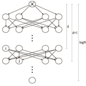
Figure 6 illustrates theorem 2. In the first testing round after an event at node a, the sons of node a diagnose the event. In the second testing round the nodes that are sons of node a’s sons diagnose the event, either by getting information from the sons of node a or by testing node a
directly. After d testing rounds, node i with diagnostic distance equal to d to node a diagnose the event. Finally the node with the largest diagnostic distance to node a,
log 2 N, diagnoses the event, in at most log 2 N testing rounds.
Figure 6. Illustration of TFFa.
Theorem 3. The maximum number of tests required by all fault-free nodes in one testing round is O(N3).
Proof:
Initially, consider only one fault-free node in the system and N–1 faulty nodes. To complete the diagnosis of the system, the fault-free node sends tasks to the faulty nodes combining then in pairs, so the number of tests executed is the combination of N–1 in pairs: .
However these tests are not enough for the fault-free node to achieve the complete diagnosis, so the fault-free node assumes that it is itself fault-free and sends tasks to itself and each one of the other nodes, i.e. it executes N–1 more tests. Thus the total number of tests required by one fault-free node is:
Now consider two fault-free nodes. The maximum number of tests required by these two fault-free nodes is at most two times the maximum number of tests required for one fault-free node. The number of tests executed in this case is:
For three fault-free nodes, the theoretical maximum number of tests required is three times the maximum number of tests required for one fault-free node:
, that is O(N3).
It is known that as more nodes are fault-free less tests are required to complete the diagnosis, because the fault-free nodes can get diagnostic information from other fault-free nodes. For example, when all N nodes are
fault-free, each node executes
tests, which are smaller
than
. Although the worst case is extremely rare
it is O(N 3).
5. SIMULATION RESULTS
In this section experimental results obtained with
Hi-Comp’s simulation are presented. The simulations were conducted using the discrete event simulation language SMPL [26]. Nodes were modeled as SMPL facilities, and each node was identified by a SMPL token number. Three types of events were defined: test, fault and repair.
Results of two experiments are presented. The first experiment shows the worst case of the latency, whose results confirm theorem 1. In the second experiment we investigated the maximum number of tests for different numbers of fault-free nodes, from 1 node to N–1 nodes; this experiment shows the difference between the simulated maximum number of tests required and the theoretical maximum presented in theorem 2.
5.1 ALGORITHM’S LATENCY
To illustrate the algorithm’s latency two experiments are presented: the first one considers the diagnosis of one event. In this experiment all nodes are fault-free, then an event happens in one node. In the second experiment, we consider the diagnosis of N–1 simultaneous events, initially only one node is fault-free, then one event happens in each faulty node and all nodes of system become fault-free, the experiment shows how the node that was fault-free from the beginning diagnoses all events.
5.1.1 DIAGNOSISOF 1 EVENT
The purpose of this experiment is illustrate the amount of testing rounds needed for one event to be diagnosed by all the other N–1 fault-free nodes, in a system of 16 nodes.
Figure 7. System of 16 nodes with one event.
By the definition of testing round, each node running the algorithm must obtain diagnostic information about all nodes of the system in each testing round, i.e., a node k is tested, at least, by all nodes of which node k is son in each testing round.
Thus in the first testing round after an event on node k, all nodes of which node k is son diagnose this event. In the second testing round after the event, the information about the event is passed to the testers of the sons of node k and the information flows through TFFi
graph.
Table 1. Number of nodes that diagnoses an event per testing round in a system of 16 nodes.
This experiment was conducted over the system of 16 nodes shown in figure 7. The event happens in node 15 and the information about this event must be passed on until node 0 receives the information. Table 1 shows the amount of nodes that diagnose the event in each testing round. In the first testing round after the event, 4 nodes diagnoses the event, in the second round 6 nodes, in the third round other 4 nodes and in the fourth round only 1 node diagnoses the event.
5.1.2 DIAGNOSISOFN–1 SIMULTANEOUS EVENTS
Figure 8. 16 nodes system with N–1 faulty nodes.
In the first testing round after the events, node 0 diagnoses the events that occurred at its sons, as all the other nodes do. In the second testing round node 0 diagnoses the events that occurred at the sons of its sons through its sons, and son on until the entire system is diagnosed.
Table 2 shows the amount of events node 0 diagnoses per testing round.
Table 2. Amount of nodes that node 0 diagnoses per testing round, in a system of 16 nodes with 15
simultaneous events.
So, in log216 = 4 testing rounds after the events, node 0 correctly diagnoses all events.
5.2 MAXIMUM NUMBER
OF TESTSThe purpose of this experiment is to show the maximum number of tests performed by different amounts of fault-free nodes in one testing round. In this experiment, all arrangements of fault-free nodes were analyzed and the ones with the largest number of tests per testing rounds were picked, from 0 to N fault-free nodes.
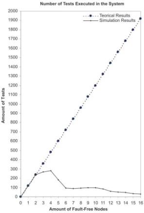
Figure 9. Number of tests executed in the system.
In figure 9 the continuous line depicts the number of tests executed in the system for the different amounts of fault-free nodes; the dashed line shows the theoretical worst case of the number of tests according to theorem 3. As shown in the figure, the real number of tests required is smaller than the theoretical maximum number of tests predicted in theorem 3.
As shown in figure 10 the largest amount of tests occurs when there are only four fault-free nodes in the system. In Hi-Comp a node executes tests in the system until it finds two fault-free nodes. Nodes were arranged as shown in figure 10; this situation forces all fault-free nodes to execute the largest number of tests to find two fault-free nodes. For example, node 0 needs to test all nodes between nodes 1 and 14, sending tasks to each pair of nodes in this interval, until tests the pair formed by nodes 1 and 14. All fault-free nodes repeat this situation, raising the number of tests to its maximum.
This results confirm the suspicion that the maximum number of tests in the system is less than O(N 3).
6. CONCLUSION
This paper presented the distributed comparison-based model in which the Hi-Comp (Hierarchical Comparison-based Adaptive Distributed System-Level Diagnosis) algorithm is based. This is the first hierarchical, distributed and comparison-based algorithm.
Nodes running comparison-based diagnosis algorithms execute tests by comparing tasks results. In Hi-Comp nodes must test other nodes to achieve the complete diagnosis. A tester sends a task to two nodes. Each of these nodes executes this task and sends its output to the tester. The tester receives and compares the two outputs; if the comparison produces a match, the tester assume that the two nodes are fault-free; but, if the comparison produces a mismatch, the tester considers that, at least one of the two nodes is faulty, but cannot identify which one.
When a fault-free node is tested, the tester obtains diagnostic information about the entire cluster of the tested node. Clusters contain N/2 nodes. To allow nodes to determine the order in which events were detected, the algorithm employs timestamps.
The new algorithm’s latency is log2N testing rounds. A testing round is defined as the period of time that all fault-free nodes need to obtain diagnostic information about all nodes of the system.
The maximum number of tests in the system is O(N3)
tests per testing round. The algorithm is N–1-diagnosable, i.e., if there are up to N–1 faulty nodes in the system, the fault-free nodes still achieve the complete correct diagnosis.
A practical tool for faulty management of computer networks applications based on the Hi-Comp algorithm is one of the main objectives for future work.
REFERENCES
[1] A. Subbiah, and D.M. Blough, “Distributed Diagnosis in Dynamic Fault Environments,” IEEE Transactions on Paralel and Distributed Systems, Vol. 15 No. 5, pp. 453-467, 2004.
[2] G. Masson, D. Blough, and G. Sullivan, “System Diagnosis,” Fault-Tolerant Computer System Design, ed. D.K. Pradhan, Prentice-Hall, 1996. [3] F. Preparata, G. Metze, and R.T. Chien, “On The
Connection Assignment Problem of Diagnosable Systems,” IEEE Transactions on Electronic Computers, Vol. 16, pp. 848-854, 1968.
[4] S.L. Hakimi, and A.T. Amin, “Characterization of Connection Assignments of Diagnosable Systems,” IEEE Transactions on Computers, Vol. 23, pp. 86-88, 1974. [5] S.L. Hakimi, and K. Nakajima, “On Adaptive System
Diagnosis,” IEEE Transactions on Computers, Vol. 33, pp. 234-240, 1984.
[6] S.H. Hosseini, J.G. Kuhl, and S.M. Reddy, “A Diagnosis Algorithm for Distributed Computing Systems with Failure and Repair,” IEEE Transactions on Computers, Vol. 33, pp. 223-233, 1984.
[7] E.P. Duarte Jr., and T. Nanya, “A Hierarchical Adaptive Distributed System-Level Diagnosis Algorithm,”
IEEE Transactions on Computers, Vol.47, pp. 34-45, 1998.
[8] R.P. Bianchini, and R. Buskens, “Implementation of On-Line Distributed System-Level Diagnosis Theory,” IEEE Transactions on Computers, Vol. 41, pp. 616-626, 1992.
[9] A. Brawerman, and E.P. Duarte Jr., “A Synchronous Testing Strategy for Hierarchical Adaptive Distributed System-Level Diagnosis,” Journal of Electronic Testing Theory and Applications, Vol. 17, No. 2, pp. 185-195, 2001.
[10] E.P. Duarte Jr., A. Brawerman, and L.C.P. Albini, “An Algorithm for Distributed Hierarchical Diagnosis of Dynamic Fault and Repair Events,” Proc. IEEE ICPADS’00, pp. 299-306, 2000.
[11] S. Lee, and K.G. Shin, “Probabilistic Diagnosis of Multiprocessor Systems,” ACM Computing Surveys, Vol. 26, No. 1, pp. 121-139, 1994.
[12] M. Malek, “A Comparison Connection Assignment for Diagnosis of Multiprocessor Systems,” Proc. Seventh Int’l Symp. Computer Architecture, pp. 31-36, 1980.
[13] K.Y. Chwa, and S.L. Hakimi, “Schemes for Fault-Tolerant Computing: A Comparison of Modularly Redundant and t-Diagnosable Systems,”
[15] A. Sengupta, and A.T. Dahbura, “On Self-Diagnosable Multiprocessor Systems: Diagnosis by Comparison Approach,” IEEE Transactions on Computers, Vol. 41, No. 11, pp. 1386-1396, 1992.
[16] D.M. Blough, and H.W. Brown, “The Broadcast Comparison Model for On-Line Fault Diagnosis in Multicomputer Systems: Theory and Implementation,” IEEE Transactions on Computers, Vol. 48, pp. 470-493, 1999.
[17] D. Wang, “Diagnosability of Hipercubes and Enhanced Hypercubes under the Comparison Diagnosis Model,” IEEE Transactions on Computers, Vol. 48, No. 12, pp. 1369-1374, 1999. [18] G.S. Almasi, and A. Gottlieb, Highly Parallel
Computing, The Benjamim/Commings Publishing Company Inc., 1994.
[19] C. Xavier, and S.S. Iyengar, Introduction to Parallel Algorithms, Wiley-Intersciense Publication, 1998. [20] N.F. Tzeng, and S. Wei, “Enhanced Hypercubes,”
IEEE Transactions on Computers, Vol. 40, No. 3, pp. 284-294, Mar. 1991.
[21] T. Araki, and Y. Shibata, “Diagnosability of Butterfly Networks under the Comparison Approach,” IEICE Trans. Fundamentals, Vol E85-A, No. 5, Maio 2002. [22] F.T. Leighton, Introduction to Parallel Algorithms and Architectures: Arrays, Trees, Hypercubes, Morgan Kaufmann, San Mateo, CA, 1992.
[23] J. Fan, “Diagnosability of Crossed Cubes,” IEEE Transactions on Computers, Vol. 13, No. 10, pp. 1099-1104, Out. 2002.
[24] F. Harary, Graph Theory, Addison-Wesley Publishing Company, 1971.
[25] S. Rangarajan, A.T. Dahbura, and E.A. Ziegler, “A Distributed System-Level Diagnosis for Arbitrary Network Topologies,” IEEE Transactions on Computers, Vol. 44, No. 2, pp. 312-333, 1995. [26] M.H. MacDougall, Simulating Computer Systems: