Zooplankton community structure in the Yellow Sea and East China Sea in
autumn
Study on zooplankton spatial distribution is
essential for understanding food web dynamics in
marine ecosystems and ishery management. Here
we elucidated the composition and distribution of
large mesozooplankton on the continental shelf of
the Yellow Sea and East China Sea, and explored
the zooplankton community structure in these water
masses. Sixty vertical hauls (bottom or 200 m in
deep water to surface) using a ring net (diameter
0.8 m, 505-μm mesh) were exploited in November
2007. The biogeographic patterns of zooplankton
communities were investigated using multivariate
analysis methods; copepod biodiversity was
analyzed using univariate indices. Copepods and
protozoans were dominate in the communities.
Based on the species composition, we divided
the study areas into six station groups. Signiicant
differences in zooplankton assemblages were
detected between the Yellow Sea and East China
Sea. Species richness was higher in East China Sea
groups than those in Yellow Sea, whereas taxonomic
distinctness was higher in Yellow Sea than in East
China Sea. There was a clear relationship between
the species composition and water mass group.
A
bstrAct
Hongju Chen
1,2, Guangxing Liu
1,2,*
1 Key Laboratory of Marine Environment and Ecology, Ministry of Education (Ocean University of China).
(Qingdao, 266100, P. R. China)
2 College of Environmental Science and Engineering, Ocean University of China.
(Qingdao, 266100, P. R. China)
*Corresponding author: [email protected]
Financial Support: This study was supported by the National Key Basic Research Project (2014CB953700) and National Natural Science Foundation of China (41210008, 31101875).
Descriptors:
Zooplankton, Community composition,
Taxonomic distinctness, Environmental factors, East
China Sea, Yellow Sea.
O estudo da distribuição espacial do zooplancton é
essencial para o entendimento não só da dinâmica das
teias tróicas nos ecossistemas marinhos, mas também
para o manejo da pesca. Neste trabalho procuramos
elucidar a composição e distribuição do
mesozoo-plancton na plataforma continental do Mar Amarelo e
do Mar da China Oriental, e explorar a estruturas das
comunidades nessas duas massas de água. Sessenta
arrastos verticais (do fundo ou de 200m até a
superfí-cie) foram realizados em Novembro de 2007, usando
uma rede circular com diâmetro de 0,8m e malhagem
de 505µm. Os padrões biogeográicos das
comunida-des do zooplancton foram investigados, utilizando-se
métodos de análise multivariada. A biodiversidade de
Copepoda foi analisada através de indices
univaria-dos. Copéodes e protozoários foram os organismos
dominantes nas amostragens. Baseados na
composi-ção de espécies, pudemos dividir a área de estudo em
seis grupos de estações. Diferenças signiicantes nas
assembléias de zooplancton foram detectadas entre o
Mar Amarelo e o Mar da China Oriental. A riqueza de
espécies foi mais elevada nesta última área, enquanto
a distinção taxonômica foi mais alta no Mar Amarelo.
Houve uma clara relação entre composição de
espé-cies e tipo de massa de água.
r
esumo
Descritores: Zooplancton, Composição da
comu-nidade, Distinção taxonômica, Mar da China Leste, Mar Amarelo.
INTRODUCTION
Zooplankton constituted by diverse marine organisms play an important role in energy transfer in marine food webs (MACKAS; TSUDA, 1999). They feed on bacteria, phytoplankton, other zooplankton, detritus (or marine snow) and even nektonic organisms, serving as a basic food source for larval and juvenile ishes as well as carnivorous invertebrates (MACKAS; TSUDA, 1999; FIELDING et al., 2007). The distribution of zooplankton in abundance or biomass terms is greatly inluenced by the hydrographic conditions (WOODD-WALKER, 2002; BERASATEGUI et al., 2005) and have been suggested to be good biological indicators for water masses (ZHENG et al., 1989; HSIEH et al., 2004). Knowledge of zooplankton distributions in a spatial scale is fundamental for understanding the plankton ecology, ishery management and the mechanisms by which physical and biological processes build marine ecosystems (HITCHCOCK et al., 2002).
The Yellow Sea and East China Sea are connected waters surrounded by mainland China, the Korean Peninsula, Kyushu Island, Ryukyu Islands, and Taiwan Island with an area of about 1.17 × 10⁶ km2, of which over 70% is on the continental shelf. As marginal seas in the northwestern of Paciic Ocean, the Yellow Sea and East China Sea have special circulation systems. On one hand, as they are greatly inluenced by oceanic Kuroshio currents, the current systems of these seas bear deep-sea characteristics with great stability. On the other hand, the climate and great river discharges affect the shallow marginal seas, giving current systems shallow-shelf characteristics subject to frequent disturbances. The circulation pattern in this area is a cyclonic system composed of the northward Kuroshio Current and the southward Coastal Current (SU, 1989). The most fundamental water masses in this area include the Coastal Water, Yellow Sea Water, Mixed Water, and Kuroshio Water (SU, 1989; FENG et al., 1999). The presence of bodies of water from different origins brings about the complexity of hydrographic characteristics in this region. The spatial distribution pattern of zooplankton in the shelf is believed to be affected by these complicated water properties.
Zooplankton studies in this area have mainly been focused on special taxonomic components, such as foraminiferans (CHENG; CHENG, 1960), medusae (XU; LIN, 2006a), ostracods (LIN et al., 1998), copepods (SHIH; CHIU, 1998; ZUO et al., 2006), and tunicates
(XU; ZHANG, 2006c; XU et al., 2007), or regional areas, such as the Yellow Sea (ZUO et al., 2003), East China Sea (CHENG, 1965; CHEN et al. 1980), and the Kuroshio area (LIU et al., 1991). Very few studies have been reported on the distribution pattern of zooplankton in the whole shelf (ZUO et al., 2005; CHEN et al., 2011). ZUO et al. (2005) analyzed zooplankton community classiications on the shelf area of the East China Sea and Yellow Sea based on two surveys in spring and autumn. They found results that differed from previous studies conducted in local sea areas (CHENG, 1965; CHEN et al., 1980). CHEN et al. (2011) reported community classiication results of the Yellow Sea and East China Sea in summer and winter. Despite the availability of such studies, however, the large-scale pattern of zooplankton community distributions in the East China Sea and Yellow Sea remains unclear, especially in the shelf area of the East China Sea.
We conducted therefore a comprehensive investigation covering the whole continental shelf of the Yellow Sea and East China Sea in autumn of 2007. Based on the net zooplankton samples obtained (large mesozooplankton fraction (SIEBURTH et al., 1978), we examined the abundance, presence of different assemblages and biodiversity as well as their relationships with environmental variables. The major objectives of this study were to 1. to elucidate the zooplankton community structure on the continental shelf of the Yellow Sea and East China Sea and 2. to explore the relationship between the their features and the water masses. It is believed that this study contributes signiicantly to research on plankton ecology in the east China coastal seas.
MATERIAL AND METHODS
Sampling procedure
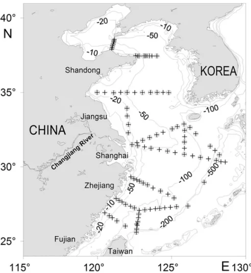
A total of 100 oceanographic stations were set, and integrated zooplankton samples were obtained from 60 stations in the Yellow Sea and East China Sea in 1st~25th
November 2007 on board R/V “Dong-Fang-Hong 2” (Figure 1). Zooplankton were sampled by a 0.8 m diameter, 505 μm mesh ring net hauled vertically from near the sea bottom (or 200 m in deep water) to the sea surface at a rate between 0.8 and 1 m·s-1. Nets were washed after each tow, and the samples were preserved in 5% formalin (inal concentration in seawater) for further analyses.
Figure 1. Map of the study area showing the positions of the oceanographic (+) and biological (○) stations, with
isobaths of 10, 20, 50, 100, 200, and 500 m.
subsample was obtained from each sample using a Folsom plankton splitter. The volume of each subsample was determined according to the density of organisms in the original sample to include at least 200 adult individuals. Data were standardized to abundance per cubic meter based on the theoretical estimation considering iltered water volume determined from the rope length multiplied with the mouth size.
Temperature, conductivity, and water depth data were obtained using a CTD proiler (Sea-Bird SBE 9, Sea-Bird Electronics, Inc.).
Data analysis
Multivariate analysis
Data were analyzed using the statistical package Plymouth Routines In Multivariate Ecological Research (PRIMER v6.1.10, PRIMER-E Ltd., 2006) (CLARKE;
(depth, temperature, and salinity) accounted for patterns in the species data. The BVSTEP routine was used to test for redundancy in the taxonomic dataset by checking if a limited subset of species could produce the same pattern.
Univariate analysis on copepod biodiversity
Taxa richness is represented by the number of species. In this study, taxa richness of each single station (SRs) and station group (SRg) deined by cluster analysis was calculated. Sample evenness was calculated using Pielou’s evenness J’ (PIELOU, 1975).
WARWICK & CLARKE (1995) deined an index of taxonomic diversity, Δ, which captures the structure not only of the distribution of abundance among species but also the taxonomic relatedness of taxa in each sample. This index was calculated as follows:
Δ =
where Xi is the abundance of the ith species and ωij is the
distinctness weight linking species or genera, in this case i
and j. For this analysis, two species at the greatest taxonomic
distance apart was set to ω = 100. Thus, the path between species was ωspecies = 25, ωgenera = 50, ωfamily = 75, ωorder = 100.
In the absence of a genetic phylogeny, the published morphological phylogenetic tree for copepods (HUANG, 1994) was used to calculate taxonomic distinctness (Δ*) (CLARKE; WARWICK, 1998).
Δ*=
For the above analyses, the PRIMER v6 package (see CLARKE; WARWICK, 2001) was used.
Differences in biodiversity indexes between zooplankton communities (deined by the cluster analysis) were tested using one-way ANOVA and followed by Student-Newman-Keuls post-hoc multiple comparison tests (SPSS 11.5).
RESULTS
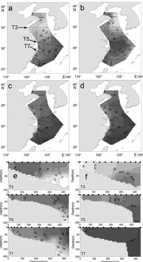
Hydrography
The surface and bottom distribution of temperature and salinity are shown in Figure 2. Surface temperatures ranged from 14.8 ºC to 26.0 ºC, whereas bottom
temperatures (or 200 m in deepwater) ranged from 8.8 ºC to 22.6 ºC. Surface salinity ranged from 25.5 to 34.5, whereas bottom salinity (or 200 m in deepwater) ranged from 25.9 to 34.7. Decreasing gradients of both surface and bottom temperatures were detected from the south to the north. The bottom temperature values indicate the presence of Cold Water in the Yellow Sea during the survey time (Figure 2b). Salinity gradually increased from north to south and from inshore to offshore.
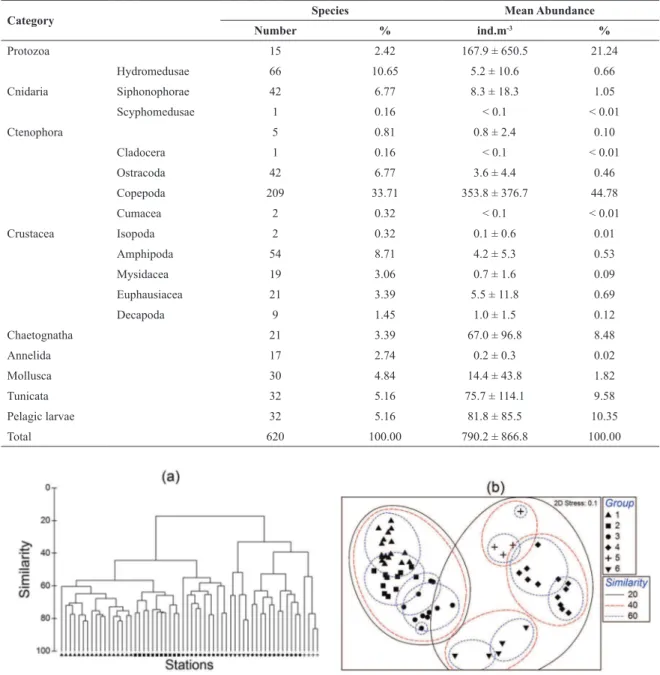
Species composition and abundance
A total of 588 taxa, and 32 planktonic larvae taxa were identiied (Table 1) (Annex, link: http://www.io.usp.br/ index.php/arquivos/send/328-vol-63-no-4-2015/3839-anexo). The plankton taxa richness and mean abundance are shown in Table 1. Crustaceans were the most abundant component among the identiied groups, representing > 55% and 45% of the total species richness and abundance, respectively. Copepods were the dominant organisms (209 taxa, mean abundance of 353.8 ind.m-3), followed by protozoans (15 taxa, mean abundance of 167.9 ind.m-3). Planktonic larvae included polychaete larvae, Ophiopluteus, and Calyptopis, etc.
Community structure
A total of 50 out of 620 less numerically represented taxa were used for multivariate analyses. Results of hierarchical cluster analyses and multi-dimensional scaling are shown in Figures 3a and 3b. Two-dimensional MDS plots divided the sixty stations into six groups (G1 to G6), with each group containing 17, 11, 11, 12, 4, and 5 stations, respectively (Figure 3b).
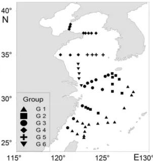
The station groups showed strong geographic integrity when overlaid on the survey area (Figure 4). G1 occupied the offshore area of the East China Sea and was inluenced directly by the Kuroshio water mass. Stations belonging to G2 were found in the middle regions of the East China Sea, where the Kuroshio branch current mixed with the coastal current. Group G3 was located in the coastal region of the East China Sea and adjacent areas off the Changjiang River estuary. Group G4 was located in the northwestern region of the Yellow Sea. Stations belonging to G5 were located in the middle region of the Yellow Sea. Group G6 was located in the coastal region of Jiangsu Province and the Changjiang River estuary. Mean zooplankton abundance in G4 was higher than in any other group, and the abundance of G6 was the lowest (Table 2 and Figure 5) among the groups found.
, 2 / ) 1 ( 2 / ) 1 ( 0
∑∑ < +∑ −
∑∑ < +∑ −
iXi Xi j
i XiXj
i Xi Xi j
i ωijXiXj
.
∑ ∑ < ∑ ∑ < ∑
j
i XiXj
j
Figure 2. Horizontal and vertical distribution of temperatures (ºC) and salinity: (a) surface temperature, (b) bottom
Table 1. Zooplankton species richness and average abundance (ind.m-3) of each category.
Category Species Mean Abundance
Number % ind.m-3 %
Protozoa 15 2.42 167.9 ± 650.5 21.24
Cnidaria
Hydromedusae 66 10.65 5.2 ± 10.6 0.66
Siphonophorae 42 6.77 8.3 ± 18.3 1.05
Scyphomedusae 1 0.16 < 0.1 < 0.01
Ctenophora 5 0.81 0.8 ± 2.4 0.10
Cladocera 1 0.16 < 0.1 < 0.01
Ostracoda 42 6.77 3.6 ± 4.4 0.46
Copepoda 209 33.71 353.8 ± 376.7 44.78
Cumacea 2 0.32 < 0.1 < 0.01
Crustacea Isopoda 2 0.32 0.1 ± 0.6 0.01
Amphipoda 54 8.71 4.2 ± 5.3 0.53
Mysidacea 19 3.06 0.7 ± 1.6 0.09
Euphausiacea 21 3.39 5.5 ± 11.8 0.69
Decapoda 9 1.45 1.0 ± 1.5 0.12
Chaetognatha 21 3.39 67.0 ± 96.8 8.48
Annelida 17 2.74 0.2 ± 0.3 0.02
Mollusca 30 4.84 14.4 ± 43.8 1.82
Tunicata 32 5.16 75.7 ± 114.1 9.58
Pelagic larvae 32 5.16 81.8 ± 85.5 10.35
Total 620 100.00 790.2 ± 866.8 100.00
Figure 3. Identiication of station groups based on the results of (a) Bray-Curtis Clustering and (b) non-metric MDS ordination both using data
from station matrix.
The statistical routine ANOSIM was used to test differences between the station groups. The null hypothesis of no differences between groups was rejected by the global R statistic (R = 0.893), and values of R in all pairwise comparisons were > 0.674 (p < 0.001). The
station groups derived from clustering were shown to be robust ways of grouping the data.
The species responsible for similarities within and dissimilarities between groups in 50 taxa that were used for multivariate analyses were detected by analysis of
similarity (SIMPER). The mean abundance of the taxa that contributed ≥ 3% to within-group similarity or between-group dissimilarity are summarized in Table 3. The listed taxa accounted for >90% of within-group similarity across all groups.
Figure 4. Distribution of station groups derived from station ordination.
Table 2. Zooplankton abundance (ind.m-3) by station grouping.
Station group (nº sites)
Mean
abundance S.D.
G1 (17) 618.7 346.6
G2 (11) 836.6 652.7
G3 (11) 571.7 718.8
G4 (12) 1301.9 1569.4
G5 (4) 973.5 1095.8
G6 (5) 377.6 188.8
Figure 5. Distribution of total zooplankton abundance (ind.m-3) by
station.
warm and tropical species, such as Scolecithricella longispinosa, Clausocalanus furcatus, Oikopleura longicauda, and Oncaea venusta, as well as neritic species,
such as Paracalanus aculeatus and Calanus sinicus. Differences were primarily accounted for by the variation of abundance of each species in different groups (Table 3). Note that except for the taxa used for multivariate analyses, a large number of typical tropical-oceanic species (e.g.,
Euchirella spp., Undeuchaeta spp., Xanthocalanus spp., Scolecithricella spp., Oncaea spp., Sapphirina spp.,
and Copilia spp.) and deep-sea species (e.g., Haloptilus mucronatus, and Arietellus setosus) were recorded in
G1. G4 was characterized by high abundance and mainly dominated by Noctiluca scintillans, Aidanosagitta crassa,
and C. sinicus. G5 encompassed stations occurring in the
middle region of the Yellow Sea and was distinguished from all other groups by a high abundance of C. sinicus, P. parvus, and Oithona similis. G6 was characterized by low
abundance and mainly comprised neritic and oligohaline species like P. aculeatus, Labidocera euchaeta, and Pesudeuphausia sinica.
The smallest subset of taxa in the matrix that could explain most of the patterns in the data was identiied by the PRIMER routine BVSTEP. The routine identiied a subset of 12 of the original 50 species/taxa in the matrix (ρ = 0.950). All 12 species were previously determined to strongly contribute to the within-group similarity and between-group dissimilarity (Table 3). These species led to much of the variation between station groups, and their distributions are presented in Figure 6.
Twelve species were common to the SIMPER and BVSTEP analyses. The distribution patterns of these species were divided into three types: (A) those only appearing in the northern coastal area such as L. euchaeta
and N. scintillans; (B) those widespread and abundant in
the north of the surveyed area such as C. sinicus and P. parvus; and (C) other taxa that varied in abundance and
only appeared in the south.
Table 3. Mean abundance (ind.m-3) summed across all groups by station grouping of those species/taxa that contributed ≥ 3% to within-group similarity or between-group dissimilarity. Highest mean values are in boldface.
Species/taxa Mean Abundance (ind.m
-3)
G1 G2 G3 G4 G5 G6
Acartia negligens 9.6 ± 6.9 1.6 ± 2.0 0.1 ± 0.1 0 0 0
Acartia paciica 0.1 ± 0.2 1.6 ± 2.1 17.1 ± 23.1 0.4 ± 0.9 1.8 ± 2.5 20.0 ± 17.3 Acrocalanus gracilis 22.5 ± 22.8 10.7 ± 8.1 2.1 ± 2.5 0 0 0
Bivalve larvae 1.4 ± 2.1 3.7 ± 6.9 1.0 ± 1.5 17.0 ± 26.4 0.5 ± 0.5 1.1 ± 1.9 Calanus sinicus 5.4 ± 8.9 8.5 ± 13.6 38.7 ± 71.9 96.8 ± 87.3 162.9 ± 47.9 15.9 ± 11.0 Calyptopis larvae 3.8 ± 3.7 10.4 ± 8.0 9.0 ± 8.2 2.1 ± 4.4 0.1 ± 0.2 20.0 ± 19.2
Canthocalanus pauper 8.8 ± 6.4 17.7 ± 11.9 8.7 ± 5.6 0 0.1 ± 0.1 0.1 ± 0.2 Clausocalanus arcuicornis 16.9 ± 15.0 13.8 ± 11.9 1.4 ± 2.2 0 0 0 Clausocalanus furcatus 14.2 ± 14.6 67.5 ± 91.3 2.1 ± 3.6 0 < 0.1 0
Corycaeus afinis < 0.1 0.2 ± 0.4 1.3 ± 2.0 36.6 ± 102.0 0.6 ± 0.4 5.6 ± 6.3 Diphyes chamissonis 0.5 ± 1.1 3.6 ± 5.0 19.4 ± 28.0 0.3 ± 0.8 0.1 ± 0.0 4.5 ± 3.6 Doliolum denticulatum 7.0 ± 8.4 2.9 ± 2.6 2.3 ± 6.7 46.4 ± 72.4 3.2 ± 4.4 0
Subeucalanus subcrassus 7.5 ± 10.3 4.1 ± 5.0 18.8 ± 25.4 0 < 0.1 0 Euchaeta copepodite 30.7 ± 28.8 39.5 ± 30.6 66.4 ± 69.8 < 0.1 12.6 ± 12.9 1.9 ± 3.9 Globigerinoides sacculifera 20.8 ± 18.6 8.2 ± 12.2 0 0 0 0
Labidocera euchaeta 0 0 0 0.2 ± 0.1 0 18.3 ± 23.9 Limacina trochiformis 8.6 ± 23.6 38.1 ± 78.6 0.4 ± 0.7 0 0 0 Noctiluca scintillans 0 < 0.1 3.0 ± 7.8 727.5 ± 1403.6 0 45.9 ± 49.2
Oikopleura dioica 0.2 ± 0.4 1.8 ± 6.1 1.1 ± 2.6 16.7 ± 28.1 18.2 ± 25.8 5.0 ± 3.7 Oikopleura fusiformis 10.2 ± 8.7 3.1 ± 6.8 < 0.1 0 0 0 Oikopleura longicauda 83.6 ± 85.7 65.8 ± 136.0 6.1 ± 6.5 30.1 ± 89.1 < 0.1 < 0.1
Oikopleura rufescens 9.7 ± 10.4 0.5 ± 1.1 0.3 ± 0.6 0.3 ± 1.1 0 0 Oithona plumifera 16.9 ± 13.4 31.8 ± 23.7 7.8 ± 10.5 0.9 ± 2.0 65.3 ± 31.3 0 Oithona similis 0 0.2 ± 0.4 0.1 ± 0.5 0.3 ± 0.8 269.9 ± 534.2 0
Oncaea venusta 21.0 ± 28.7 72.9 ± 84.6 8.8 ± 10.7 0 0.2 ± 0.2 0 Ophiopluteus larvae 34.8 ± 49.2 10.0 ± 16.3 18.4 ± 34.9 6.7 ± 15.8 0 33.7 ± 64.3 Paracalanus aculeatus 31.1 ± 31.6 97.6 ± 64.5 81.6 ± 57.5 0 13.6 ± 17.1 118.6 ± 132.4
Paracalanus gracilis 8.4 ± 19.4 61.8 ± 113.7 3.2 ± 10.5 0 0 0 Paracalanus parvus 0.2 ± 0.5 8.3 ± 12.4 26.9 ± 31.1 75.9 ± 85.4 367.0 ± 577.6 3.6 ± 7.4 Pesudeuphausia sinica 0 0 1.8 ± 2.1 < 0.1 < 0.1 9.0 ± 8.7
Radiolarian 8.9 ± 11.2 10.0 ± 10.7 0 0 0 0
Zonosagitta bedoti 1.3 ± 1.9 10.2 ± 6.4 32.2 ± 43.2 0 0 0 Aidanosagitta crassa 0 0.1 ± 0.2 < 0.1 164.7 ± 144.5 17.2 ± 12.2 15.2 ± 38.7
Flaccisagitta enlata 16.4 ± 13.0 12.8 ± 6.4 26.4 ± 28.0 1.5 ± 2.5 2.8 ± 1.2 0.8 ± 1.1 Sagitta nagae 0.1 ± 0.2 1.1 ± 1.2 5.8 ± 10.2 19.0 ± 17.6 8.7 ± 4.3 20.6 ± 12.3 Scolecithricella longispinosa 4.2 ± 8.8 21.3 ± 14.2 47.7 ± 65.1 0 0 < 0.1
Undinula vulgaris 10.9 ± 8.7 27.1 ± 27.7 1.8 ± 3.2 0 0.1 ± 0.0 0
undertaken to test the correspondence and signiicance of environmental data to the station groupings. The best it was obtained from the combination of surface temperature and bottom salinity (ρ= 0.836), and the best it of a single
Figure 6. Distribution and abundance (ind.m-3) of each species (a. Noctiluca scintillans; b. Labidocera euchaeta; c. Calanus sinicus; d. Paracalanus parvus; e. Paracalanus aculeatus; f. Canthocalanus pauper; g. Undinula vulgaris;
h. Scolecithricella longispinosa; i. Subeucalanus subcrassus; j. Clausocalanus furcatus; k. Acrocalanus gracilis; l. Globigerinoides sacculifera).
Figure 7. Variations in depth, temperature, and salinity in different
station groups.
Univariate analysis on copepod biodiversity
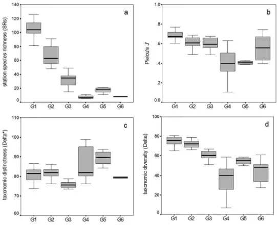
A total of 209 pelagic copepod species from 61 genera, 28 families, and 4 orders were found in 60 samples. Calanoid copepods were the most abundant components. SRg values varied dramatically, and corresponding valuesfor G1, G2, G3, G4, G5, and G6 were 189, 137, 88, 18, 29 and 15, respectively.
All copepod biodiversity indexes showed signiicant differences (p < 0.001) between groups derived from
station ordination according to one-way ANOVA. However, post-hoc multiple comparison tests indicated that mean SRs values among G4, G5, and G6 show no signiicant difference (Figure 8a). The value of J’ between
Figure 8. The distribution of (a) station taxa richness (SRs), (b) evenness (Pielou’s J'), (c) taxonomic distinctness (Δ*), and
(d) taxonomic diversity (Δ) of copepods among station groups. Boxes display the median, 25th, and 75th percentiles, and the
error bars denote 10th and 90th percentiles.
DISCUSSION
Faunistic areas
Marine environments with different oceanographic features support plankton fauna with different species compositions. Researchers have ubiquitously detected the association between water masses and species communities in other sea areas (WARD et al., 2004; MARRARI et al., 2004; BERASATEGUI et al., 2005). In the present study, the BIOENV routine clearly associated zooplankton distribution patterns with environment factors; a clear relationship between zooplankton assemblages and water mass distributions was also detected. Signiicant differences in zooplankton communities were detected between the Yellow Sea and East China Sea (Figures 3 and 4).
The Yellow Sea is a temperate semi-closed shallow sea characterized by neritic and warm temperate species. This sea area is not inluenced by the Kuroshio system except its southeast part. G4 (corresponding to Yellow Sea Water) was located in the northwestern coastal region of the Yellow Sea and dominated and characterized by
N. scintillans, A. crassa, and Doliolum denticulatum. The Cold Water of the Yellow Sea was observed even in autumn because of remnant stratiication from summer (Figure 2). G5 was located in the middle region of the Yellow Sea and greatly controlled by the Yellow Sea Cold Water. This group was dominated and characterized by low-temperature, high-salinity, and widely distributed warm-temperate species such as C. sinicus, P. parvus, O. similis, and O. plumifera. G6 (corresponding to Subei
Coastal Water) was located in the coastal region of Jiangsu Province (Lusi ishing grounds) and extended to the Changjiang River estuary. This group was characterized by neritic or eurythermal low-salinity species such as L. euchaeta, P. sinica, and P. aculeatus.
corresponded to East China Sea Surface Water. G3 was a coastal community located in the coastal region of the East China Sea as well as adjacent areas off the Changjiang River estuary; this group corresponded to East China Sea Coastal Water. Zooplankton biodiversity showed an obvious gradient from the inshore to offshore areas.
CHENG (1965) found four planktonic communities in the Yellow Sea, namely the Liaoning Coastal Community, the Shandong Coastal Community, the Yellow Sea Central Community, and the northern Jiangsu Coastal Community. Upon comparison of these communities with the zooplankton faunistic areas identiied in the present study, we found a similar general trend; however, the resolution of the present study was low because of the limited number of sampling stations employed. Thus, we could not differentiate the Liaoning and Shandong Coastal Communities from the Yellow Sea Community.
The present faunistic areas identiied concurred with previous studies on the zooplankton distribution in the East China Sea shelf (LIU et al., 1991; LIN et al.,1998). ZUO et al. (2005) concluded that East China Sea zooplankton fauna in autumn comprised the East China Sea Inshore Mixed Water Community and the East China Sea Shelf Mixed Water Community; these results differ from those found in the present study.
A parallel pattern was detected when we compared the results of the present study with summer and winter results (CHEN et al., 2011). The boundaries of different communities shifted with changes in hydrographic conditions in different seasons. In the previous study, in summer we detected a Changjiang Estuary assemblage in the station located at the mouth of the Changjiang River, and the surface salinity was low (21.6 psu; CHEN et al., 2011). In autumn and winter, it was dificult to distinguish the Changjiang Estuary assemblage from the coastal community as a result of the Changjiang River discharge decrease. Compared with that of summer and winter (CHEN et al., 2011), the coastal community (G3) extended in the north of the East China Sea in autumn, and infringed the space of the mixed-water community (G2). The mixed-water community was clearly reduced in the spatial scope in autumn.
Species occurrence and distribution
A total of 588 taxonomic categories (not including planktonic larvae) were recorded in this survey, and the taxa richness was much higher than that recorded in some other sea areas worldwide such as the Scotia
Sea (120 taxonomic categories, WARD et al., 2004), southwestern Atlantic Ocean (27 taxa, MARRARI et al., 2004), northern California Current area (85 taxa, REESE et al., 2005), and the Iberian shelf (107 taxa, CABAL et al., 2008). Decreasing taxa richness and evenness were detected from offshore to inshore areas and from south to north. Only 50 taxa among the 620 categories found were subjected to multivariate analyses; most of the species excluded from the analyses exist in the Kuroshio area with low abundance. The zooplankton community in the Kuroshio area is characterized by high taxa richness and low abundance (SHIH; CHIU, 1998). Researchers have proposed that the thermal structure provides a greater number of niches for zooplankton in tropic and subtropic (Kuroshio) areas (RUTHERFORD et al., 1999; WOODD-WALKER et al., 2002) and that production cycles are of generally low amplitude all year round, which leads to a retentive system in which diversity is characteristically high (WOODD-WALKER et al., 2002).
Zooplankton composition and abundance showed signiicant differences between station groups. The dominant taxa mainly included protozoans, copepods, tunicates, chaetognaths, and medusae. (Tables 1 and 3).
Copepods
Copepods were the most abundant taxon, and their dominance was conirmed throughout the survey area (Table 3); this taxon accounted for 17%-91% of the total abundance of each group. C. sinicus, Paracalanus, Clausocalanus, Oithona, and O. venusta were found
to be dominant, and C. sinicus was the most signiicant
species. Similar indings have been observed in previous studies (CHENG et al., 1965; ZUO et al. 2006; CHEN et al., 2011). C. sinicus is a copepod widely distributed
in the Northwestern Paciic continental shelf. The highest abundance of C. sinicus may be found in the Yellow Sea,
and numbers of the organism decrease gradually toward the south and offshore areas (Figure 6). These results support the inding that C. sinicus prefers to live in waters
with relatively low temperatures (HUANG et al., 1993). The distribution pattern of the small copepod species P. parvus was similar to that of C. sinicus.
L. euchaeta is a species widely distributed in China seas
(HUANG, 1994) that lives in habitats with salinity lower than 30 (ZHU, 1988). L. euchaeta was the most important species
Other copepod species identiied by routine BVSTEP mainly appeared in the East China Sea, but their distribution patterns varied signiicantly. The highest abundance of P. aculeatus and Canthocalanus pauper,
for example, was distributed in the inshore area and middle part of East China Sea (G2, G3); in the Kuroshio area, however, their abundance was relatively low. The high abundance of Undinula vulgaris and C. furcatus
were mainly distributed in mixed water areas (G2). XU (2006a) reveals that U. vulgaris is a warm-water species.
The high abundance of U. vulgaris could be used as a
good indicator of warm currents. In this study, a small amount of U. vulgaris extended to the south Yellow Sea,
which reveals that the south Yellow Sea is inluenced by the incursion of warm currents. A decreasing gradient of the abundance of S. longispinosa and Subeucalanus subcrassus was detected from inshore to offshore areas,
and the abundance of Acrocalanus gracilis was higher in
the southern and offshore areas than in the northern and inshore areas.
Meso-small pelagic copepods, such as P. parvus, P. aculeatus, C. furcatus, A. gracilis, and S. longispinosa,
were important dominant species in this study. These copepods play a crucial role in marine ecosystem (SÁNCHEZ-VELASCO, 1998; NIP et al., 2003). The present study was carried out using samples collected by 505 μm mesh plankton nets, and mainly focused on zooplankton with body sizes > 500 μm. Such a procedure could underestimate observable taxa richness because many species with body sizes < 500 μm were not fully represented or neglected (MAKABE et al., 2012). The 50 taxa subjected to the multivariate analyses might changed signiicantly if a smaller mesh net were used. Besides, in the present study, the volume of water was determined from rope length multiplied with net mouth size. This method was just a theoretical estimation. In this case, there might be an overestimation of water volume iltered by the net, and consequently aggravate the underestimation of zooplankton. In future work, zooplankton studies in China seas could be conducted with nets < 200 μm or smaller to avoid underestimation of smaller organisms and understand the zooplankton community structure more thoroughly. Moreover, lowmeter should be used for calculating the quantity of water iltered by the net.
The present results showed that at low latitudes and high sea surface temperatures sea areas for instance G1 and G2, the copepod taxonomic diversity (Δ) was higher. G1 and G2 were similar in taxonomic composition (average dissimilarity, 43.39; SIMPER analysis) and mainly dominated by widely distributed warm and tropical species (e.g., C. pauper, U. vulgaris, P. gracilis, A. gibber, A. gracilis, C. arcuicornis, C. furcatus, and O. venusta).
Differences were primarily accounted for by the abundance variation of each species in different groups, and the abundance of G2 was higher than that of G1 (Table 3).
The distribution patterns of biodiversity parameters adopted in this study varied dramatically (Figure 8), but similar results have been recorded in other sea areas (BERASATEGUI et al., 2005). The biodiversity distribution changed depending on which index was being calculated. We found an increase in taxonomic distinctness in the Yellow Sea, which indicates a longer mean path distance through the taxonomic tree connecting every pair of species despite the lower taxa richness. The measured value of taxonomic richness should theoretically be smaller than in actual conditions because of the net mesh size. The taxonomic diversities Δ* and Δ can provide more
intuitive and comprehensive measures of biodiversity than other conventional indices, as these parameters are relatively insensitive to the disparities in sampling effort (WARWICK; CLARKE, 1998, 2001).
Protozoans
As a well-known bloom-forming zooplankton, N. scintillans is an opportunistic omnivorous species. The
rapid reproduction capability of this species, together with its polyphagous feeding behavior, enables N. scintillans outbursts in populations under favorable
conditions (YILMAZ et al.; 2005). In the present study,
N. scintillans was the most abundant protozoan species,
mainly appearing in the northern coastal area. In G4, N. scintillans contributed 55.9% of the total abundance.
Globigerinoides sacculifera was the second most
important protozoan species. Contrasted to the distribution of N. scintillans, G. sacculifera, was only found in
foraminifera in the Yellow Sea and East China Sea and demonstrated that its high abundance is only distributed south of 29ºN. Our result supports the conclusion of CHENG & CHENG (1960), that the southwestern sea area of Jeju Island is the northernmost distribution extension for G. sacculifera.
Other species
A total of 109 cnidarian medusa species were recorded in this survey. The total medusa abundance was low despite of its high species richness. Three dominant species, Aglaura hemistoma, Nanomia bijuga,
and Diphyes chamissonis, were all warm-temperate and
mainly distributed in East China Sea.
Chaetognaths were generally abundant throughout the survey area and classiied as important. A. crassa, S. nagae, and F. enlata were the most abundant species.
Chaetognath species richness was low, with A. crassa
dominating the Yellow Sea. A. crassa was the most
important chaetognath species in the Bohai and Yellow Seas, and its abundance gradually decreased from the north to the south; this species was absent in East China Sea. The number of chaetognatha in the East China Sea was far more than that in the Yellow Sea.
O. dioica and O. longicauda were the dominant
species among the Appendicularians. O. dioica was
mainly distributed in the Yellow Sea and in the inshore areas of East China Sea. O. longicauda showed broad
adaptability and was distributed in almost all of the seas with high frequency. Thalia democratica orientalis was
concluded to be the most important Thaliacea species in China seas (ZHENG et al., 1989). However, the present study showed that D. denticulatum is the dominant
Thaliacea component.
We provided broad spatial coverage of the east marginal seas of China and comprehensive information on the abundance and distribution of zooplankton dominant groups as well as organisms of less signiicance. Our results contribute to a better understanding of the community structure and biodiversity of the area.
REFERENCES
BERASATEGUI, A. D.; RAMÍREZ, F. C.; SCHIARITI, A. Patterns in diversity and community structure of epipelagic copepods from the Brazil-Malvinas Conluence area, south-western Atlantic. J. Mar. Syst., v. 56, n. 3/4, p. 309-316, 2005.
CABAL, J.; GONZÁLEZ-NUEVO, G.; NOGUEIRA, E. Mesozooplankton species distribution in the NW and N Iberian shelf during spring 2004: Relationship with frontal structures. J. Mar. Syst., v. 72, n. 1/4, p. 282-297, 2008. CHEN, H. J.; QI, Y. P.; LIU, G. X. Spatial and temporal variations
of macro- and mesozooplankton community in the Huanghai Sea (Yellow Sea) and East China Sea in summer and winter. Acta. Oceanol. Sin., v. 30, n. 2, p. 84-95, 2011.
CHEN, Q. C.; CHEN, Y. Q.; HU, Y. Z. Preliminary study on the plankton communities in the southern Yellow Sea and the East China Sea. Acta. Oceanol. Sin., v. 2, n. 2, p. 149-157, 1980. (in Chinese with English Abstract).
CHENG, T. C. The structure of zooplankton communities and its seasonal variation in the Yellow Sea and in the western East China Sea. Oceanol. Limnol. Sin., v. 7, n. 3, p. 199-204, 1965. (in Chinese with English Abstract).
CHENG, T. C.; CHENG, S. Y. The planktonic Foraminifera of the Yellow Sea and the East China Sea. Oceanol. Limnol. Sin., v. 3, n. 3, p. 125-156, 1960. (in Chinese with English Abstract)
CLARKE, K. R.; WARWICK, R. M. A taxonomic distinctness index and its statistical properties. J. Appl. Ecol., v. 35, p. 523-531, 1998.
CLARKE, K. R.; WARWICK, R. M. Change in marine communities: an approach to statistical analysis and interpretation. 2nd. ed. Plymouth: PRIMER-E, 2001. FENG, S. Z.; LI, F. Q.; LI, S. J. An introduction to marine science.
Beijing: Higher Education Press, 1999.
FIELD, J. G.; CLARKE, K. R.; WARWICK, R. M. A practical strategy for analyzing multi-species distribution patterns. Mar. Ecol. Prog. Ser., v. 8, p. 37-52, 1982.
FIELDING, S.; WARD, P.; POULTON, A. J.; POLLARD, R. T.; SEEYAVE, S.; READ, J. F.; HUGHES, J. A.; SMITH, T.; CASTELLANI, C. Community structure and grazing impact of mesozooplankton during late spring/early summer 2004/2005 in the vicinity of the Crozet Islands (Southern Ocean). Deep Sea Res. Part II., v. 54, p. 2106-2125, 2007.
HITCHCOCK, G. L.; LANE, P.; SMITH, S.; LUO, J.; ORTNER, P. B. Zooplankton spatial distributions in coastal waters of the northern Arabian Sea, August, 1995. Deep Sea Res. Part II., v. 49, n. 12, p. 2403-2423, 2002.
HSIEH, C. H.; CHIU, T. S.; SHIH, C. T. Copepod diversity and composition as indicators of intrusion of the Kuroshio branch current into the northern Taiwan Strait in spring 2000. Zool. Stud., v. 43, n. 2, p. 393-403, 2004.
HUANG, C.; UYE, S.; ONBE, T. Ontogenetic diel vertical migration of the planktonic copepod Calanus sinicus in the Inland Sea of Japan III. Early summer and overall seasonal pattern. Mar. Biol., v. 117, n. 2, p. 289-299, 1993.
HUANG, Z. G., ed. Marine species and their distributions in China seas. Beijing: Ocean Press, 1994. p. 496-516. LIN, J. H.; CHEN, R. X.; GUO, F. F. Ecological of Ostracoda in
LIU, H. B; HE, D. H.; WANG, C. S. Preliminary study on distributions and communities of zooplankton in the Kuroshio area of the middle-southern East China Sea. In: Essays on the investigation of Kuroshio. Beijing: Ocean Press, 1991. p. 305-313. (in Chinese)
MACKAS, D. L.; TSUDA, A. Mesozooplankton in the eastern and western subarctic Paciic: community structure, seasonal life histories, and interannual variability. Prog. Oceanogr., v. 43, n. 2/4, p. 335-363, 1999.
MAKABE, R.; TANIMURA, A.; FUKUCHI, M. Comparison of Mesh Size Effects on Mesozooplankton Collection Eficiency in the Southern Ocean. J. Plankton Res., v. 34, n. 5, p. 432-436, 2012.
MARRARI, M.; VIÑAS, M. D.; MARTOS, P.; HERNÁNDEZ, D. Spatial patterns of mesozooplankton distribution in the Southwestern Atlantic Ocean (34º-41ºS) during austral spring: relationship with the hydrographic conditions. ICES J. Mar. Sci., v. 61, p. 667-679, 2004.
NIP, T. H. M.; HO, W.; WONG, C. K. Feeding ecology of larval and juvenile black seabream (Acabthopagrus schlegeli) and Japanese seaperch (Lateolabrax japonicus) in Tolo Harbour, Hong Kong. Environ. Biol. Fish., v. 66, p. 197-209, 2003. PIELOU, E. C. Ecological Diversity. New York: John Wiley and
Sons, 1975. 165 p.
REESE, D. C.; MILLER, T. W.; BRODEUR, R. D. Community structure of near-surface zooplankton in the northern California Current in relation to oceanographic conditions. Deep Sea Res. Part II., v. 52, n. 1/2, p. 29-50, 2005. RUTHERFORD, S.; D’HONDT, S.; PRELL, W. Environmental
controls on the geographic distribution of zooplankton diversity. Nature, v. 400, p. 749-753, 1999.
SÁNCHEZ-VELASCO, L. Diet composition and feeding habits of ish larvae of two co-occurring species (Pisces: Callionymidae and Bothidae) in the North-western Mediterranean. ICES J. Mar. Sci., v. 55, n. 2, p. 299-308, 1998.
SHIH, C. T.; CHIU, T. S. Copepod diversity in the water masses of the southern East China Sea north of Taiwan. J. Mar. Syst., v. 15, n. 1, p. 533-542, 1998.
SIEBURTH, J. M. C. N.; SMETACEK, V.; LENZ, J. Pelagic ecosystem structure: Heterotrophic compartments of the plankton and their relationship to plankton size fractions. Limnol. Ocenogr., v. 23, p. 1256-1263, 1978.
SU, Y. S. A survey of geographical environment circulation system in the Huanghai Sea and East China Sea. J. Ocean. Univ. Qingdao, v. 19, n. 1, p. 145-158, 1989. (in Chinese, with English Abstract).
WARD, P.; GRANT, S.; BRANDON, M.; SIEGEL, V. Mesozooplankton community structure in the Scotia Sea during the CCAMLR 2000 survey: January-February 2000. Deep Sea Res. Part II, v. 51, p. 1351-1367, 2004.
WARWICK, R. M.; CLARKE, K. R. New “biodiversity” measures reveal a decrease in taxonomic distinctness with increasing stress. Mar. Ecol. Prog. Ser., v. 129, p. 301-305, 1995.
WOODD-WALKER, R. S.; WARD, P.; CLARKE, A. Large-scale patterns in diversity and community structure of surface water copepods from the Atlantic Ocean. Mar. Ecol. Prog. Ser., v. 236, p. 189-203, 2002.
XU, Z. L. Relationships between population characters of Undinula vulgaris (Copepoda) and environment in the East China Sea. Chin. J. Appl. Ecol., v. 17, n. 1, p. 107-112, 2006a. (in Chinese with English Abstract).
XU, Z. L.; LIN, M. Causal analysis on diversity of Medusa in the East China Sea. Biodivers. Sci., v. 14, p. 508-516, 2006b. (in Chinese with English Abstract).
XU, Z. L.; LIN, M.; ZHANG, J. B. Relationship of water environment and abundance distribution of Thaliacea in the East China Sea. Oceanol. Limnol. Sin., v. 38, n. 6, p. 549-554, 2007. (in Chinese with English Abstract).
XU, Z. L.; ZHANG, F. Y. Species distribution and diversity of Appendicularia in the East China Sea. J. Shanghai Fish. Univ., v. 15, n. 3, p. 286-291, 2006c. (in Chinese with English Abstract)
YILMAZ, I. N.; OKUS, E.; YÜKSEK, A. Evidences for inluence of a heterotrophic dinolagellate (Noctiluca scintillans) on zooplankton community structure in a highly stratiied basin. Estuar. Coast. Shelf. Sci., v. 64, n. 2/3, p. 475-485, 2005. ZHENG, Z.; LI, S. J.; XU, Z. Z. Marine Planktology. Berlin
Heidelberg, New York, Tokyo, Beijing: China Ocean Press & Springer-Verlag, 1989.
ZHU, Q. Q. An investigation on the ecology of zooplankton in Changjiang Estuary and Hangzhou Bay. J. Fish. Chin., v. 12, n. 2, p. 111-123, 1988. (in Chinese with English Abstract) ZUO, T.; WANG, R.; CHEN, Y. Q.; WANG, K. Net
macro-zooplankton community classiication on the shelf area of the East China Sea and the Yellow Sea in spring and autumn. Acta. Ecol. Sin., v. 25, n. 7, p. 1531-1540, 2005. (in Chinese with English Abstract)
ZUO, T.; WANG, R.; CHEN, Y. Q.; GAO, S. W.; WANG, K. Autumn net copepod abundance and assemblages in relation to water masses on the continental shelf of the Yellow Sea and East China Sea. J. Mar. Syst., v. 59, n. 1/2, p. 159-172, 2006. ZUO, T.; WANG, R.; WANG, K.; GAO, S. W. Multivariate