On the Shelf Resonances of the Gulf of Carpentaria and the Arafura Sea

(1)

OSD

9, 443–497, 2012

Gulf of Carpentaria Resonances

D. J. Webb

Title Page

Abstract Introduction

Conclusions References

Tables Figures

◭ ◮

Back Close

Full Screen / Esc

Printer-friendly Version Interactive Discussion

Discussion

P

a

per

|

Dis

cussion

P

a

per

|

Discussion

P

a

per

|

Discussio

n

P

a

per

|

Ocean Sci. Discuss., 9, 443–497, 2012 www.ocean-sci-discuss.net/9/443/2012/ doi:10.5194/osd-9-443-2012

Ocean Science Discussions

This discussion paper is/has been under review for the journal Ocean Science (OS). Please refer to the corresponding final paper in OS if available.

On the Shelf Resonances of the Gulf of

Carpentaria and the Arafura Sea

D. J. Webb

National Oceanography Centre, Southampton SO14 3ZH, UK

Received: 20 December 2011 – Accepted: 6 January 2012 – Published: 3 February 2012 Correspondence to: D. J. Webb ([email protected])

(2)

OSD

9, 443–497, 2012

D. J. Webb

Title Page

Tables Figures

◭ ◮

Back Close

Full Screen / Esc

Discussion

P

a

per

|

Dis

cussion

P

a

per

|

Discussion

P

a

per

|

Discussio

n

P

a

per

|

Abstract

A numerical model is used to investigate the resonances of the Gulf of Carpentaria and the Arafura Sea. The model is forced at the shelf edge, first with physically real-istic real values of angular velocity. The response functions at points within the region show maxima and other behaviour which imply that resonances are involved but it is 5

difficult to be more specific. The study is then extended to complex angular veloci-ties and the results then show a clear pattern of gravity wave and Rossby wave like resonances. The properties of the resonances are investigated and used to reinter-pret the responses at real values of angular velocity. It is found that in some regions the response is dominated by modes trapped between the shelf edge and the coast 10

or between opposing coastlines. In other regions the resonances show cooperative behaviour, possibly indicating the importance of other physical processes.

1 Introduction

Recent studies by Arbic et al. (2009) and Green (2009) have again highlighted the question of the extent to which barotropic resonances affect the response of the ocean 15

to external forcing. Because of their shape and bathymetry, one might expect to see resonances in both the deep ocean and the shelf seas. Both are of interest but the shelf resonances may be particularly important because of their potential impact on tidal power generation.

One can make a first estimate of the number of deep ocean resonances from studies 20

such as that of Longuet-Higgins and Pond (1980). They calculated the resonant modes of a series of hemispherical oceans of uniform depth. Taking the ocean to have an av-erage depth of 4000 m their results show that such an ocean would have eight resonant modes between one and two cycles per day (2πand 4πradians per day)1the density

1

(3)

OSD

9, 443–497, 2012

D. J. Webb

Title Page

Tables Figures

◭ ◮

Back Close

Full Screen / Esc

Discussion

P

a

per

|

Dis

cussion

P

a

per

|

Discussion

P

a

per

|

Discussio

n

P

a

per

|

of modes increasing rapidly as the angular velocity increases. Platzman et al. (1981) investigated the resonances of a more realistic ocean and found 14 modes in the same band of frequencies. They also found a greater density of resonances at and beyond 4πradians per day.

As the tidal bands themselves have a width of approximately one radian per day 5

one might expect to see the evidence of such modes in the tidal records. In contrast the analysis of tidal records, such as those discussed by Munk and Cartwright (1966), indicate that with the possible exception of the Coral Sea region (Webb, 1973b), the response of the ocean is usually very smooth.

One possible explanation for this is that frictional effects are so strong that the res-10

onances are damped out. This is consistent with a number of independent estimates of the residence of tidal energy in the ocean, that the decay time is of order 30 h or less (Miller, 1966; Garrett and Munk, 1971; Webb, 1973a; Egbert and Ray, 2003). The equivalent decay time for the wave amplitude is twice this.

Bottom friction acting in the deep ocean is too small to produce such a rapid decay 15

and the traditional view was that the energy was lost on continental shelves. Later studies of satellite data (e.g. Egbert and Ray, 2001) show that a significant amount of tidal energy is lost to internal tides along mid-ocean ridges and other topographic features. However this is still less than the amount being lost on the shelves.

The loss of energy to the shelves was investigated by Webb (1976) who found that 20

a tidal wave approaching a coastline from the deep ocean tended to be reflected back into the deep ocean with very little energy being lost on the continental shelf. Excep-tions were found to occur when the shelf is near resonance, i.e. when it is 1/4, 3/4 etc. wavelengths wide, but if the friction is too small or two large, the tidal energy is still reflected back into the deep ocean. Thus a shelf will only have a significant ef-25

fect in dissipating tidal energy if it has both the right dimensions and the right frictional properties.

(4)

OSD

9, 443–497, 2012

D. J. Webb

Title Page

Tables Figures

◭ ◮

Back Close

Full Screen / Esc

Discussion

P

a

per

|

Dis

cussion

P

a

per

|

Discussion

P

a

per

|

Discussio

n

P

a

per

|

Although this, and the more recent work of Arbic et al. (2009) on the coupling of the shelf sea modes to the deep ocean, gives us some confidence in the results, our understanding of the shelf sea resonances is still very limited. With this in mind the present paper reports some work on the response functions and resonances of the Gulf of Carpentaria and the Arafura Sea.

5

The area has been chosen for a number of reasons. First it enables use of a model which has been validated in a study of both the diurnal and semi-diurnal tides of the region (Webb, 1981). Thus the model should give good results over the whole band of frequencies around one and two cycles per day.

Secondly it is a large continental shelf. It therefore might be expected to show many 10

of the resonance features to be found elsewhere. Previously Buchwald and Williams (1975) investigated the resonances of the region using a simpler model and it is also of interest to compare results from the two types of model.

Thirdly, related to point two, tidal observations indicate that in the north of Arafura Sea the region contains a classic quarter wavelength resonance. Tidal heights are 15

smaller than those found in the classic resonance regions, such as the Bay of Fundy and the Bristol Channel, but it does provide an opportunity to learn more about such resonances.

Finally, and most importantly, the validated model is not limited to studies with real angular velocities. It also allows investigation of the complex angular velocity plane 20

where each of the resonances produces a mathematical pole with an infinite response. This allows the properties of individual resonances to be investigated. Each reso-nance’s contribution to the response of the real ocean can then be calculated and their interactions further studied.2

2

(5)

OSD

9, 443–497, 2012

D. J. Webb

Title Page

Tables Figures

◭ ◮

Back Close

Full Screen / Esc

Discussion

P

a

per

|

Dis

cussion

P

a

per

|

Discussion

P

a

per

|

Discussio

n

P

a

per

|

2 The numerical model

A numerical model is used to solve Laplace’s tidal equations. In vector notation and with a linear friction term these are,

∂u_/∂t₊f×u₊₍_κ/h₎u₊_g∇_ζ ₌_g∇_ζ_eq_, ₍₁₎

∂ζ /∂t+∇ ·₍_hu)=0.

5

u_{is the depth averaged horizontal velocity,} _t _{is time,}_ζ _{the sea level,}_ζ_eq _{the height of}

the equilibrium tide (corrected for Earth tides),gthe acceleration due to gravity, κ the linear friction coefficient, hthe depth and “×_{” indicates a vector product. The Coriolis}

vectorf _{is defined by,}

f₌₂_Ω_cos(_θ₎n_z_, ₍₂₎

10

whereΩis the Earth’s rotation rate, θthe co-latitude, and n_z _{the unit vertical vector.}

The equations are obtained by integrating the full equations of motion in the vertical and neglecting the vertical acceleration, non-linear and self-attraction terms.

Equation (1) is linear, so the general solution for a given forcing can be written as a linear combination of solutions of the form,

15

_u

(t)

ζ(t)

=ℜ_[

_u

ζ

exp(−_{i ωt}_)]_, ₍₃₎

whereωis the angular velocity andℜ_{represents the real part of the complex}

expres-sion.

If we defineP andQ_as,

P =g(i ω−_κ/h₎_/_[(_{i ω}−_κ/h₎2₊_f2_]_, ₍₄₎

20

Q₌f_/[(i ω−_κ/h₎2₊_f2_]_,

then,

(6)

OSD

9, 443–497, 2012

D. J. Webb

Title Page

Tables Figures

◭ ◮

Back Close

Full Screen / Esc

Discussion

P

a

per

|

Dis

cussion

P

a

per

|

Discussion

P

a

per

|

Discussio

n

P

a

per

|

where,

ζ′=ζ−_ζ_eq_. ₍₆₎

Substituting foru_{in Eq. (1),}

hP∇2_ζ′₊_[∇₍_hP₎₊∇ ×₍_hQ_)]· ∇_ζ′ 1

−_{i ωζ}′₌_{i ω ζ}_eq_. ₍₇₎

5

This is the equation that is solved numerically in the model.

At coastlines the normal component of velocity is zero as the model depth there is required to be non-zero. Ifnc is the unit vector normal to the coast, then from Eq. (5),

(P+Q×₎∇_ζ′·n_c₌₀_. ₍₈₎

3 Numerical solution 10

In the numerical model, the spherical co-ordinate form of Eq. (7) is replaced by a set of finite difference equations at the vertices of a rectangular grid, using a grid spacing of one eighth of a degree. The boundary condition, Eq. (8), is applied at points where the grid intersects coastlines, the finite difference equations taking into account both the angle between the coastline and the grid and the curvature of the coastline. Both 15

coastline and depths were taken from Admiralty charts of the region.

In the original model (Webb, 1981), observed values of the tidal height were imposed on the open boundaries to the west of the Arafura Sea and on the eastern side of Torres Strait. For the new study reported here the wave entering the region from the west is assumed to have unit amplitude and constant phase all along the western boundary. 20

In the east, Torres Strait is now blocked.

(7)

OSD

9, 443–497, 2012

D. J. Webb

Title Page

Tables Figures

◭ ◮

Back Close

Full Screen / Esc

Discussion

P

a

per

|

Dis

cussion

P

a

per

|

Discussion

P

a

per

|

Discussio

n

P

a

per

|

not have constant phase but the effect is likely to be small. In the east the original tidal study (Webb, 1981) showed that the amount of tidal energy entering through Torres Strait is small and has little effect on the tides within the Gulf. As a result the revised boundary condition, which simplifies the analysis, should have little effect on the large scale response of the region.

5

The coefficients resulting from the finite difference equations are loaded into a sparse matrix and the associated forcing terms into a corresponding vector. The full matrix equation is then solved using Gaussian elimination and back substitution, the num-bering of the vertices being organised to minimise the size of the intermediate matrix. Further details of the model and solution are given in Webb (1981).

10

4 The behaviour at tidal frequencies

Figures 2 and 3, reproduced from Webb (1981), show the original model’s solution for the K1 and M2 tides. In the figures, the amplitude and phase lines are from the model and the boxed figures show the same quantities measured at tide gauges. There are discrepancies but they are relatively small.

15

The K1 amplitude and phase lines indicate that, to a first approximation, the diurnal tide propagates along the northern boundary as a Kelvin wave and that it then circles clockwise around the Gulf of Carpentaria losing energy on the way. However a sim-ple decaying Kelvin wave would have an amplitude which declined monotonically with distance. Instead the model shows four regions where the amplitude at the coast is a 20

local maximum.

Three of these, in corners of the Gulf may result from the Kelvin wave propagating around a nearly right-angled corner. The fourth, in the north-east of the Arafura Sea, near 138◦ E 7◦ S, could be associated with a quarter wave resonance between the Digoel River3and the shelf edge.

25

3

(8)

OSD

9, 443–497, 2012

D. J. Webb

Title Page

Tables Figures

◭ ◮

Back Close

Full Screen / Esc

Discussion

P

a

per

|

Dis

cussion

P

a

per

|

Discussion

P

a

per

|

Discussio

n

P

a

per

|

In contrast, the semi-diurnal M2 tide shows no simple resemblance to a Kelvin wave. In the north of the Arafura Sea there appears to be a 3/4 wavelength wave, trapped between the shelf edge and the Digoel River. There are two additional maxima in the south of the Arafura Sea and the north of the Gulf, which may be related, and a low amplitude east-west oscillation in the centre and south of the Gulf.

5

These results emphasise the fact that individual tidal constituents give little insight into the physical processes involved. It is possible to repeat the analysis with other tidal constituents but the tidal bands are so narrow that little more can be learnt.

But in the present case the model is not limited to the tidal bands. It can be forced with a wide range of frequencies and so provide a wealth of additional information. 10

5 The response function

Using the new boundary conditions, the model was run at a series of frequencies between zero and 30 radians per day (∼₄_._{8 cycles per day). It is impractical to show}

co-tidal charts for all the frequencies calculated, so instead Figs. 4, 5, 6 and 7 show the response R at three stations which have been selected to illustrate a range of 15

behaviour.R is defined as,

R(x)=ζ(x)/ζb, (9)

whereζ(x) is the (complex) tidal height at position x and ζb is the tidal height on the

open boundary.

The first station is near Digoel River in the north of the Arafura Sea where both the 20

diurnal and semi-diurnal tides indicate the presence of standing waves. The second is near Karumba in the south-east of the Gulf of Carpentaria. Resonances don’t appear to be a key feature of the region but there is a strong contrast between the diurnal and semi-diurnal tides. The final point is near Yaboomba Island on the southern boundary of the Arafura Sea. The diurnal tide appears as a simple progressive wave along the 25

(9)

OSD

9, 443–497, 2012

D. J. Webb

Title Page

Tables Figures

◭ ◮

Back Close

Full Screen / Esc

Discussion

P

a

per

|

Dis

cussion

P

a

per

|

Discussion

P

a

per

|

Discussio

n

P

a

per

|

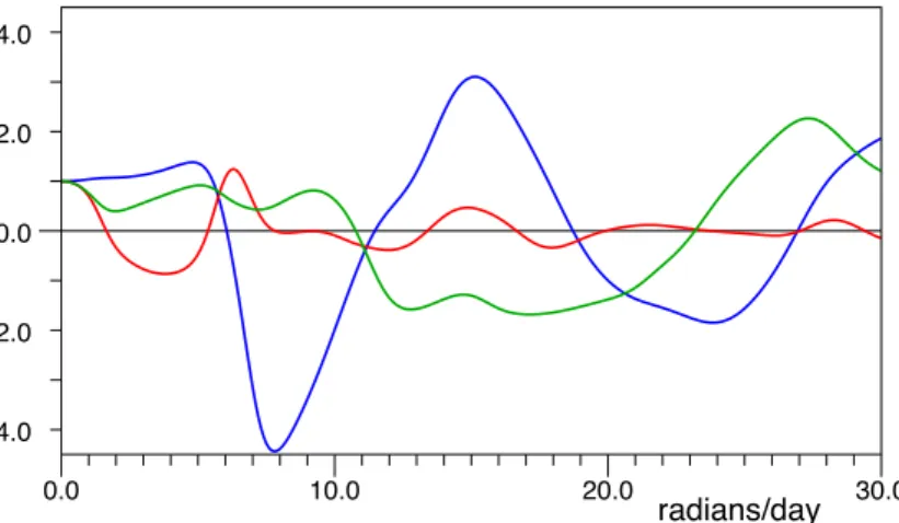
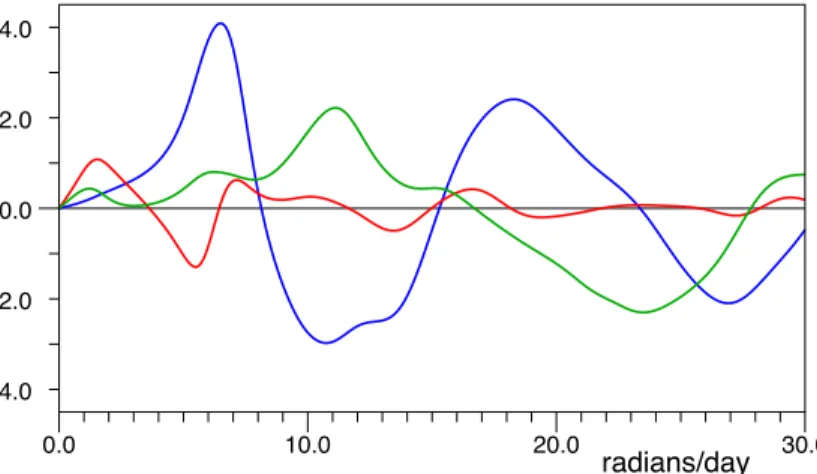
The results are presented here in three different ways. The first, in terms of the real and imaginary components ofR, is the most fundamental and is closely related to the later exploration of the complexω plane. The second, in terms of the amplitude and phase, is easier to relate to the physics and this is also true of the third, where the real and imaginary components are plotted against each other.

5

5.1 Real and imaginary components

Figures 4 and 5 show the real and imaginary components of the response function at each station. As the angular velocity tends to zero, all the real values tend to unity and the imaginary values to zero, indicating that the tide everywhere follows that on the open boundary. As the angular velocity increases the functions diverge, the Digoel 10

River showing the largest amplitude excursions. At Karumba the components have much smaller excursions, especially at higher angular velocities. Neighbouring maxima and minima are also much closer than for Digoel River.

At Yaboomba Island the oscillations in the real and imaginary components at low an-gular velocities are less than at the two other stations. However near 11.5 radians per 15

day there is a change in sign of the real component and a maximum in the imaginary component after which both components show oscillations comparible with those of Digoul River.

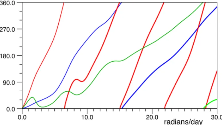
5.2 Amplitude and phase

Figures 6 and 7, replot this data in the form of the amplitude and phase of the response. 20

The amplitudes are all one at zero angular velocity but at higher values the behaviour is very different. Thus over most of the range the Digoel River amplitude is above two, it also shows very strong peaks near 7 and 14 radians per day and a weaker broader one near 27 radians per day.

The Karumba amplitude shows a small peak near 1.5 radians per day, a second one 25

(10)

OSD

9, 443–497, 2012

D. J. Webb

Title Page

Tables Figures

◭ ◮

Back Close

Full Screen / Esc

Discussion

P

a

per

|

Dis

cussion

P

a

per

|

Discussion

P

a

per

|

Discussio

n

P

a

per

|

There is a broad low peak around 13 radians per day and a further one around 30 radians per day but these are modulated by some structure which may be correlated with the Yaboomba Island response.

The Yaboomba Island station shows a third type of response. It starts low, there is a small maximum near 5.5 radians per day but after a second maximum near 11.5 radi-5

ans per day, the amplitude stays high and is comparable to that at Digoul River. The phase plots provide a different insight, in that each of the three curves tends to have a constant slope over all of the frequency range considered. There are changes in slope, on the scale of the width of the peaks in the amplitude plot, but except for these features the slope remains remarkably constant.

10

One possible way to understand this behaviour is to consider the response of a simple travelling wave,

ψ=Aexp(i kx−_{i ωt}₎_. ₍₁₀₎

Assume that the wave speed is constant so that thek equalsω/c. Then if this wave is “forced” so that it has amplitude one at the “boundary” wherexis zero, then at distance 15

x, the responseR will be simply,

R(ω)=exp(i kx), (11)

=exp(i(x/c)ω). (12)

In this case the gradient of the phase equalsx/c, the time taken for the wave to prop-agate from the boundary.

20

Applying this result to Fig. 7, it implies that on average incoming waves take about five hours to reach the Yaboomba Island from the open boundary, about ten hours to reach Digoel River and twenty-one hours to reach Karumba. The figures for Yaboomba Island and Karumba are in rough agreement what might be expected from the phase lines of Figs. 2 and 3. These indicate that, above 10 radians per day, the tidal wave 25

(11)

OSD

9, 443–497, 2012

D. J. Webb

Title Page

Tables Figures

◭ ◮

Back Close

Full Screen / Esc

Discussion

P

a

per

|

Dis

cussion

P

a

per

|

Discussion

P

a

per

|

Discussio

n

P

a

per

|

Estimates for Digoel River are complicated by the standing wave affecting the semi-diurnal tide but the semi-diurnal tide indicates about four hours which is much less than the ten hours estimated from Fig. 7. Thus the simple idea of a progressive wave appears to be too simple and an alternative picture needs to be developed.

5.3 Resonance circles 5

Webb (1973a) discusses the form of the ocean’s response to tidal forcing and shows that it has the form,

ψ(x,ω)=X j

ψ_j(x)A_j/(ω−_ω_j₎_, ₍₁₃₎

wherexdenotes position,ωis the angular velocity andω_j is the angular velocity of the j’th resonance.ψ_j(x) describes the spacial structure of the resonance andA_j depends 10

on how the system is forced.

If the resonances are well separated, then near to each resonance the function at a fixed position has the form,

ψ(ω)=Rj/(ω−ωj)+B(ω). (14)

whereB(ω) is a smooth background, the contribution of distant resonances. 15

Letω_j have real and imaginary partsω_j0andγj, whereγj is usually negative. Then

asωmoves along the real axis from minus to plus infinity, the resonance term increases from zero, to a value ofi Rj/γj, whenωequalsωj0, and returns to zero at plus infinity.

It is straight forward to show (Webb, 2011) that as this happens the real and imaginary components move anti-clockwise around a circle that starts at the origin and passes 20

throughi Rj/γj at maximum distance from the origin.

(12)

OSD

9, 443–497, 2012

D. J. Webb

Title Page

Tables Figures

◭ ◮

Back Close

Full Screen / Esc

Discussion

P

a

per

|

Dis

cussion

P

a

per

|

Discussion

P

a

per

|

Discussio

n

P

a

per

|

particular circles are also produced by delays, such as those produced by the propa-gation of progressive waves discussed in the last section, but in such cases the circles are centred on the origin.4

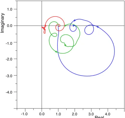
To see how well the approach works for the present results, the real and imaginary components are plotted against each other in Fig. 8. All three curves start at the 5

point (1.0+i0.0) and circle around the origin in an anti-clockwise direction. However although it is apparent that there are some underlying structures present in all three curves, only in the Yaboomba Island curve shows anti-clockwise circles and these are both very small and only occur at low angular velocities.

The main feature of the Karumba curve is that it circles the origin, initially at approx-10

imately unit distance, but finally it converges towards the origin. Thus as discussed before it appears to be primarily a progressive wave which is damped at higher angular velocities.

The Digoel River curve also circles the origin but at a distance which is much greater than one, so this cannot be a simple delay. However, in the absence of an alternative 15

explanation, it is possible that the resonances which produce the peaks of Fig. 6, are overlapping or combining in such a way as to produce an effective delay.

Figure 9 shows an attempt to remove the background by adding a linear correction to the phases, such that the total phase change over the whole band is zero. The trans-formation distorts the resonance circles, the distortion being proportional to the width 20

of the resonance and the magnitude of the linear correction (greatest for Karumba) but the effect is small when the resonances are narrow.

Now all three stations show a series of loops with a positive (anti-clockwise) curva-ture, as expected from resonances. Karumba and Yaboomba Island both show some small kinks with negative curvature but these will have been produced by the transfor-25

mation.

4

(13)

OSD

9, 443–497, 2012

D. J. Webb

Title Page

Tables Figures

◭ ◮

Back Close

Full Screen / Esc

Discussion

P

a

per

|

Dis

cussion

P

a

per

|

Discussion

P

a

per

|

Discussio

n

P

a

per

|

5.4 Analysis of real data

The results of this section show that analysis based on results with real values of the angular velocity is difficult. Plots of just the real or imaginary components as a function of angular velocity are not very useful. Peaks in the amplitude plots start to indicate the presence of resonances, three or four at Digoel River and similar numbers 5

at Yaboomba Island and Karumba but not all at the same angular velocities.

When additional confirmation is looked for in the phases, the main feature appears to be a steady changes in phase indicating, not resonances, but delays in the system. The final method, plotting the real and imaginary components against each other helps to confirm that resonances are being seen at Yaboomba Island but at the other two 10

stations interpretation is again difficult.

It is possible that if all we had was data for real values of angular velocity, then more could be learnt by fitting the plotted data to a function similar to that of Eqs. (13) or (14). However the present model can be run with complex values of angular velocity and, as is shown in the next section, this allows a more complete exploration of the complex 15

plane.

6 The Complexω_plane

Figures 10 to 12 show the real component of the response at Digoel River, Karumba and Yaboomba Island plotted as a function of complex angular velocity. The data for the figures was created by running the model at intervals of 0.1 radians per day, in both 20

the real and imaginary directions, between the origin and (30−_i_{10) radians per day.}

The data was then plotted in a view which looks beyond the real axis in the negative imaginary direction.

The values on the real axis are the same as in Fig. 6 but the direction of increasing angular velocity is now towards the left. The values in the negative real direction (not 25

(14)

OSD

9, 443–497, 2012

D. J. Webb

Title Page

Tables Figures

◭ ◮

Back Close

Full Screen / Esc

Discussion

P

a

per

|

Dis

cussion

P

a

per

|

Discussion

P

a

per

|

Discussio

n

P

a

per

|

The poles with negative imaginary values are the shelf resonances. Their positions correspond to the terms ωj in Eq. (13) and are the same in all three figures. The

apparent width of each peak is proportional to the magnitude of its residue, i.e. the termψ_j(x)A_j in the same equation. The differences between the residues in the three figures is thus a measure of the changing importance of each resonance in different 5

parts of the Gulf.

The figures show that the resonances fall into two groups with a boundary near 4 radians per day. At lower angular velocities the resonances are tightly packed and in most cases the residues are small. They resonances also have a large range of decay rates, the imaginary component of angular velocity extending to minus ten and beyond. 10

Above 4 radians per day, the resonances are well separated and have much larger residues. At the lower (real) angular velocities, the imaginary components are one to two radians per day and these increase to three to four radians per day for the resonances near 30 radians per day.

This second group of resonances is also the one which appears to have the most 15

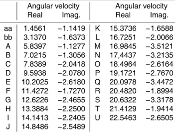
influence on the diurnal and semi-diurnal tides. Table 1 contains a list of the resonances closest to the tidal bands plus resonances with low angular velocities which appear to have most effect on the low angular velocity response at Digoel River, Karumba and Yaboomba Island.

6.1 Gravity and Rossby waves 20

Theoretical studies have shown that there are two main classes of long waves in the ocean, the gravity waves at high angular velocities, where energy is exchanged be-tween potential and kinetic energy, and the Rossby waves at low angular velocities, where the exchange is primarily an exchange of kinetic energy between the two hori-zontal components of velocity.

(15)

OSD

9, 443–497, 2012

D. J. Webb

Title Page

Tables Figures

◭ ◮

Back Close

Full Screen / Esc

Discussion

P

a

per

|

Dis

cussion

P

a

per

|

Discussion

P

a

per

|

Discussio

n

P

a

per

|

Theory also shows that the boundary between the two regimes occurs at an angular velocity off, the Coriolis parameter,

f=2Ωsin(θ), (15)

where θ is latitude and Ω is the angular velocity of the Earth. Waves with angular velocities nearf are likely to show a mixture of both properties (Longuet-Higgins, 1968; 5

Longuet-Higgins and Pond, 1980).

The Gulf of Carpentaria and the Arafura Sea span latitudes between 5◦S and 18◦S. This corresponds to values of the Coriolis parameterf, between 1.1 and 3.6 radians per day. Thus the change in properties seen near 4 radians per day can be identified as being due to the change from the Rossby wave to the gravity wave parts of the 10

spectrum.

If Eq. (1) is used to study the decay of a steady current, it is easy to show that the decay rate is proportional to κ/h, where κ is the friction parameter and h the depth. Webb (2011) investigated gravity wave resonances in a simple 1-D model with a constant depth continental shelf and showed that the resonance decay rates, the 15

imaginary parts of the complex angular velocity, were given by the same equation. In the present model, κ has the value 0.1 cm s−2 and the depths range from over 100 m in parts of the Arafura sea and 70 m in the centre of the Gulf of Carpentaria to 20 m and less near to the coastline. Using the above equation, a depth of 100 m gives a decay rate of 0.86 day−1 and this increases to 1.73 day−1for a depth of 50 m, 20

3.46 day−1 for 25 m and 8.64 day−1 for 10 m. The gravity wave values of Table 1, are thus consistent with mean depths of between 25 and 50 m, values which are not un-reasonable.

Rossby waves on a shelf of constant depth are also expected to have decay rates ofκ/h. Thus the Rossby wave resonances of the current model with decay rates of 25

(16)

OSD

9, 443–497, 2012

D. J. Webb

Title Page

Tables Figures

◭ ◮

Back Close

Full Screen / Esc

Discussion

P

a

per

|

Dis

cussion

P

a

per

|

Discussion

P

a

per

|

Discussio

n

P

a

per

|

7 The resonances

The angular velocites of the resonances can be found by fitting Eq. (14) to one of the calculated response functions in the neighbourhood of each resonance. Use was made of the four nearest calculated values and these were fitted using a linear background,

ψ(ω)=Rj/(ω−ωj)+A+B ω . (16)

5

As discussed in Appendix A, this can be converted into a linear matrix equation and so solved for the unknowns including the resonance frequencyω_j. The results for the main resonances using the data from Digoel River are given in Table 1. The results obtained from using any of the other stations are essentially the same.

Once the angular velocity of a resonance is known, the spatial structure can be cal-10

culated in a similar manner. This time solutions to the model equations were obtained for each of the four angular velocitiesω_j±_δω_and_ω

j±ıδω, whereδωequalled 0.1

ra-dian/day. Again, further details of the method used, which makes use of the properties of Vandermonde matrices, are given in Appendix A.

7.1 Resonance waveforms 15

Figures 13 to 21 show the amplitude and phase of some of the main resonances af-fecting the diurnal and semi-diurnal tides in the region. Mode aa is included because it is the fundamental quarter-wavelength mode, having a maximum at the southern limit of the Gulf of Carpentaria. However it is not a classical quarter wavelength resonance because its angular velocity is less than the Coriolis parameter everywhere except 20

near the northern coastline of the Arafura Sea. As a result its properties are those of a Rossby wave with only a small fraction of its energy in the form of potential energy. Thus even at low angular velocities it has only a limited effect on tidal height5.

5

(17)

OSD

9, 443–497, 2012

D. J. Webb

Title Page

Tables Figures

◭ ◮

Back Close

Full Screen / Esc

Discussion

P

a

per

|

Dis

cussion

P

a

per

|

Discussion

P

a

per

|

Discussio

n

P

a

per

|

The remaining resonances illustrated are all primarily gravity wave modes and as such each of them might dominate the response with a suitable pattern of forcing. However in the present case the forcing is limited to the shelf edge and this appears to limit the importance of individual resonances and they way they interact.

At low angular velocities, resonances A, B and C are well separated in angular ve-5

locity from other resonances and are relatively weakly damped. As a result one might expect them to dominate the response in the diurnal tide band and, as discussed later, this is the case.

Figures 14 and 16 show that resonances “A” and “C” are both primarily progressive waves trapped within the Gulf of Carpentaria. Their angular velocities appear to be 10

determined by “A” fitting a single wavelength around a single amphidrome and “C”, two wavelengths around a double amphidrome.

In contrast resonance “B” (Fig. 15) is primarily a quarter wavelength wave trapped between the shelf edge and the Digoel River. Some energy does propagate into and circulate around the Gulf of Carpentaria but it appears to be the distance between the 15

shelf edge and the Digoel River which determines the angular velocity of this mode. The angular velocities of resonances “B” and “C” are very close, so it is possible that this results in some mixing of the solutions.

At higher angular velocities the structure of the resonances becomes more com-plex and it is more difficult to relate them to physical features. One exception is reso-20

nance “F” which appears to be primarily a standing wave trapped between the northern boundary of the Gulf of Carpentaria and the southern boundary of the Arafura Sea. An-other is resonance “I” which is a three-quarters wave trapped between Digoel River and the shelf break. Note that this time there is very little coupling to the Gulf of Carpentaria. The remaining resonances have a more irregular structure. Many of them, like res-25

(18)

OSD

9, 443–497, 2012

D. J. Webb

Title Page

Tables Figures

◭ ◮

Back Close

Full Screen / Esc

Discussion

P

a

per

|

Dis

cussion

P

a

per

|

Discussion

P

a

per

|

Discussio

n

P

a

per

|

7.2 Comparison with a simpler model

Buchwald and Williams (1975) investigated the response of a simple rectangular gulf at the end of an infinite channel. They did not include a Coriolis term, but applying their model to the Gulf of Carpentaria, they found that the lowest resonances had periods of 16.4, 10.4 and 7.9 h (corresponding to 9.2, 14.5 and 19.1 radians per day. The results 5

were given some support by Melville and Buchwald (1976) who analysed sea level records from the Gulf of Carpenteria.

One might expect their resonances to be related to those of the present study whose energy is confined primarily to the Gulf of Carpentaria. Examples are resonances C and E, but these have angular velocities of 7.8 and 10.2 radians per day. No simple 10

relationship between the present set of resonances and the previous ones have been found. The reason for this is uncluear.

8 Resonances and real angular velocities

The polar plots, discussed earlier, showed that at real values of the angular velocity the presence of resonances could be indicated by the presence of tight loops in the 15

response function. Here use is made of this property to identify the resonances re-sponsible for the key features of the response function in the diurnal and semi-diurnal bands. Over such a band, it should be possible to expand the response functionR(x,ω) at sitexas,

R(x,ω)=X j

R_j(x)/(ω−_ω

j)+c.c.+B(x,ω), (17)

20

where the sumj is over a limited number of key resonances and B(x,ω) is a smooth background.R_j(x) andw_j are the values calculated in the previous section.

(19)

OSD

9, 443–497, 2012

D. J. Webb

Title Page

Tables Figures

◭ ◮

Back Close

Full Screen / Esc

Discussion

P

a

per

|

Dis

cussion

P

a

per

|

Discussion

P

a

per

|

Discussio

n

P

a

per

|

velocities considered, reproduced the main features of the response function and left a residual which was small and smooth.

The results are illustrated using the polar form of the response function figures. The full response function and the background term are plotted for the whole band and the individual contributions from the selected resonances and their complex conjugates are 5

plotted at two points within each band. Because of the difference in angular velocity, the complex conjugate contributions tend to be small except near zero angular velocity. Two bands of angular velocities are considered. The first extends from zero to nine radians per day. This covers the diurnal tides and also shows the behaviour at very low values of angular velocity. The second band extends from ten to fifteen radians per day 10

and covers the semi-diurnal tides.

8.1 The diurnal band

The result for Digoel River, for the band 0 to 9 radians per day is shown in Fig. 22. The large amplitude loop in the response function can all be explained by the changing am-plitude and phase of the contribution of resonance B, a quarter wavelength resonance. 15

The background term is seen to grow with angular velocity, reaching an amplitude of two by 8 radians per day but it still remains much smaller than the single resonance contribution.

The corresponding result for Karumba is shown in Fig. 23. At low angular velocities it was found necessary to include resonance “aa” in order to reduce the background at 20

near zero angular velocity. For the 5 to 8 radians per day region, which includes the diurnal tides, it was found necessary to include both “A” and “B” resonances. These both have large amplitudes and phase changes of around 90◦.

More importantly they have approximately opposite phase. Near 5 radians per day the contribution from resonance “A” is large and “B” only reduces it slightly. However 25

(20)

OSD

9, 443–497, 2012

D. J. Webb

Title Page

Tables Figures

◭ ◮

Back Close

Full Screen / Esc

Discussion

P

a

per

|

Dis

cussion

P

a

per

|

Discussion

P

a

per

|

Discussio

n

P

a

per

|

thought to be a result of an increase in the effect of friction at higher angular velocities. However in the present case both model have similar decay times and so the reduction in amplitude is purely an effect of interference between the two modes.

A further complication is found is found in the results for Yaboomba Island (Fig. 24). The first loop is found to be primarily the effect of the Rossby wave resonance “aa”. 5

Resonances “A” and “B” are also significant. They again show an approximately 90◦ phase change between 5 and 8 radians per day, but here they are acting in phase and as a result produce the increase in amplitude near 5 radians per day. Two more resonances “D” and “F” are also significant and as the angular velocity increases they grow even larger. From Figs. 17 and 19 they both involve a standing wave between 10

the southern boundary of the Arafura Sea and the north of the Gulf of Carpentaria. Together they both contribute towards completing the second loop of the response function and the further increase in its amplitude past 8 radians per day.

8.2 The semi-diurnal band

Figure 25 shows the response function at Digoel River in a range including the semi-15

diurnal tides. Resonance “B” is still significant but it is declining in importance and a large number of other resonances are now involved. These include “D”, “F”, “H” and “P”, all of which show noticeable phase changes between 11 and 14 radians per day, but the largest contribution is now from “I”, the three-quarter wave resonance trapped between the Digoel River and the shelf edge.

20

At Karumba, Fig. 26, all of the resonances in the range “D” to “K” now make sig-nificant contributions. The largest amplitude term is that of “H”, a rather complex res-onance confined to the Gulf, but its effect is to a large extent cancelled out by other resonances. However its increased amplitude does seem to be responsible for the second partial loop seen around 14 radians per day.

25

(21)

OSD

9, 443–497, 2012

D. J. Webb

Title Page

Tables Figures

◭ ◮

Back Close

Full Screen / Esc

Discussion

P

a

per

|

Dis

cussion

P

a

per

|

Discussion

P

a

per

|

Discussio

n

P

a

per

|

In contrast to Digoel River and Karumba, the number of significant resonances con-tributing to the response function at Yaboomba Island has dropped (see Fig. 27). “F” is the largest resonance, responsible for the main loop, and only two more, “D” and “F”, are required to smooth the background. The result confirms that the unusual standing wave between the southern boundary of the Arafura Sea and the northern boundary 5

of the Gulf of Carpentaria is a key feature of the region.

9 Discussion

The primary aim of the work reported has been to learn a little of the properties of resonances associated with a realistic section of continental shelf. The Gulf of Carpen-taria and Arafura Sea region was chosen because a validated model of the region was 10

available and because there were indications that resonances were present, especially in the region between the Digoel River and the shelf edge. The model also had the advantage that it could be used to investigate both real and complex values of angular velocity

The model was forced near the shelf edge and it was first used to investigate the 15

response of the region as the angular velocity varied over the tidal bands. This stage only used real angular velocities and interpretation of the results was difficult. The amplitude of the response function showed peaks but these were not simple ones that one may expect from a single resonance. The phase diagrams indicated that the wave generated by the forcing may be largely simple progressive waves which are 20

only slightly modified by some other process. However the polar diagrams showed a number of tight loops with positive curvature. Theory predicts that isolated resonances will generate such loops.

The theory of linear systems also shows that the response functions can be contin-ued as analytic functions into the complex angular velocity plane. The resonances then 25

(22)

OSD

9, 443–497, 2012

D. J. Webb

Title Page

Tables Figures

◭ ◮

Back Close

Full Screen / Esc

Discussion

P

a

per

|

Dis

cussion

P

a

per

|

Discussion

P

a

per

|

Discussio

n

P

a

per

|

The model was used to investigate the complex plane. It showed the existence of a rich pattern of resonances with a band of large poles extending from six radians per day to higher angular velocities. These were identified as the gravity wave resonances of the region. There was also a field of smaller poles with small real angular velocities but with a large range of imaginary angular velocities. These were identified as the 5

Rossby wave modes.

An investigation of the modes showed that some of the gravity modes, especially those with low (real) angular velocities, could be identified as fundamental 1/4 or 3/4 wavelength modes fitting between the shelf edge and the coast or modes associated with reflection between opposing boundaries. Others were much more complex, whose 10

main role may be to contribute to the complete set of modes needed to describe all possible waveforms within the system.

The Rossby wave modes were not investigated in the same way but one of them was found to be a 1/4 wavelength wave trapped between the shelf edge and the southern boundary of the Gulf of Carpentaria. With no Coriolis term this would be the funda-15

mental quarter wavelength mode of the system and so would have a significant impact on the sea level response. However here it is at such a low angular velocity that it is primarily a Rossby wave and, except near Yaboomba Island where the other terms are small, it has limited impact on the sea level response.

Finally, the results using real values of angular velocity were reinterpreted making 20

use of the known angular velocities and waveforms of the resonances. There are only a few resonances close to the diurnal band and these were found to dominate the response within the band. There are more resonances close to the semi-diurnal band and the behaviour there was found to be more complicated.

However the results show that in both bands there are regions where the response is 25

(23)

OSD

9, 443–497, 2012

D. J. Webb

Title Page

Tables Figures

◭ ◮

Back Close

Full Screen / Esc

Discussion

P

a

per

|

Dis

cussion

P

a

per

|

Discussion

P

a

per

|

Discussio

n

P

a

per

|

a simple progressive wave.

This apparent cooperation may simply reflect the fact that in such regions the sepa-ration between resonances is less than their distance from the real axis. Alternatively it may be an indication that, where it occurs, the physical process involved is one for which a simple resonance interpretation is the wrong one. This should occur, for ex-5

ample, in the case of a simple progressive wave. The resonance picture may also be inappropriate for a slowly narrowing channel many wavelengths long, for which a W. K. B. approximation may be more relevant. However the fact that the 1/4, 3/4 and other simple resonances stand out so clearly implies that such resonances are still likely to be important in other regions of the world’s ocean.

10

One important consideration that has not been discussed so far is the fact that the continental shelf modelled here is not connected to a realistic deep ocean. Webb (2011) investigates this problem for the simple case of a one-dimensional shelf coupled to a similar deep ocean. The results indicate that the main change is that the resonances loose some energy into the deep ocean and so they have a shorter decay 15

time (i.e. a more negative imaginary component of angular velocity). In terms of the present results, this would tend to broaden the resonances – possibly reducing their individual effects and increasing the cooperative behaviour.

A second concern is how the modes are coupled to the deep ocean resonances. As discussed by Arbic et al. (2009) one might expect the coupling to be strong only for 20

(24)

OSD

9, 443–497, 2012

D. J. Webb

Title Page

Tables Figures

◭ ◮

Back Close

Full Screen / Esc

Discussion

P

a

per

|

Dis

cussion

P

a

per

|

Discussion

P

a

per

|

Discussio

n

P

a

per

|

Appendix A

Resonance and background

The problem is to fit a series of response function valuesR(ωi) for different values of ω_i by a single resonance and a linear background,

5

R(ω_i)=R_j/(ω_i−_ω_j₎₊_P₊_{Q ω}_i_. _(A1)

P and Q are complex constants, ωj is the complex angular velocity of the resonance

andR_j its residue. This is a specific form of the more general problem of fitting a set of valuesyi andxi to an equation of the form,

y =A/(x−_B₎₊ N X

n=0

C_nxn. (A2)

10

Multiplying by (x−_B_),

y(x−_B₎₌_A₊ N X

n=0

(Cnxn+1−CnBxn), (A3)

yx=A+By−_C₀_B

+ N X

n=1

(Cn−1−CnB)xn+CNxN+1,

yx=(A−_C₀_B₎_+By

15

+ N X

n=1

(Cn−1−CnB)xn+CNxN+1.

This can be written in the form,

yx=D0y+ N+2 X

n=1

D_nxn−1_.

(25)

OSD

9, 443–497, 2012

D. J. Webb

Title Page

Tables Figures

◭ ◮

Back Close

Full Screen / Esc

Discussion

P

a

per

|

Dis

cussion

P

a

per

|

Discussion

P

a

per

|

Discussio

n

P

a

per

|

This like Eq. (A2) has N+3 unknowns. If a similar number of pairs of values x and y are available it gives a matrix equation which can be solved using standard methods for the unknownsD_{. Then,}

B=D0, (A5)

C_N =D_N₊2,

5

C_n−1=Dn+1+CnB for n=1... N , A=D1+C0B.

If, in Eq. (A1) the angular velocity of the resonanceωj is known, then Eq. (A2) can be

rewritten in the form,

y =A/x′+ N X

n=0

C_n′x′n. (A6)

10

wherex′now equals (wi−wj). Dropping the primes, the equivalent of Eq. (A4) is,

yx= N+1 X

n=0

D_nxn, (A7)

In matrix form, the set of equations become,

MD₌F_. _(A8)

whereMis a matrix andD_andF _{are vectors,}

15

Mm,n=xnm, Fm =ymxm.

Mis a Vandermonde matrix. Turner (1966) shows that its inverse,M−1, contains terms which are simple function of the variablesx_m. The solution is then given by,

D₌M−1F_. (A9)

(26)

OSD

9, 443–497, 2012

D. J. Webb

Title Page

Tables Figures

◭ ◮

Back Close

Full Screen / Esc

Discussion

P

a

per

|

Dis

cussion

P

a

per

|

Discussion

P

a

per

|

Discussio

n

P

a

per

|

The residue of the pole in Eq. (A6) is given byD0. In the case of four unknowns, if

thexis have the values±δ and±i δ, whereδ is non-zero, then the residue is just the

mean value of the elements ofF_.

Acknowledgements. I wish to thank the editors of the CSIRO journal “Marine and Freshwater Research” for permission to reuse figures from Webb (1981).

5

References

Anon: Admiralty Tide Tables, Hydrographer of the Navy, London, 1971. 472, 473

Arbic, B. K., Karsten, R. H., and Garrett, C.: On Tidal Resonance in the Global Ocean and the Back-Effect of Coastal Tides upon Open-Ocean Tides, Atmos.-Ocean, 47, 239–266, 2009. 444, 446, 465

10

Buchwald, V. T. and Williams, N. V.: Rectangular resonators on infinite and semi-infinite chan-nels, J. Fluid Mech., 67, 497–511, 1975. 446, 460

Easton, A. K.: The tides of the continent of Australia, Report 37, Horace Lamb Centre for Oceanographic Research, Flinders University of South Australia, 1988. 472, 473

Egbert, G. and Ray, R.: Estimates ofM₂tidal energy dissipation from TOPEX/Poseidon

altime-15

ter data, J. Geophys. Res., 106, 22475–22502, 2001. 445

Egbert, G. and Ray, R.: Semi-diurnal and diurnal tidal dissipation from TOPEX/Poseidon al-timeter data, Geophys. Res. Lett., 30, 1907, doi:10.1029/2003GL017676, 2003. 445 Garrett, C. and Munk, W.: The age of the Tide and the ’Q’ of the Ocean, Deep-Sea Res., 18,

493–504, 1971. 445

20

Green, J. A. M.: Ocean tides and resonances, Ocean Dynam., 60, 1243–1253, 2009. 444 Grignon, L.: Tidal resonances on the North-West European Shelf, Master’s thesis, University

of Southampton, School of Ocean and Earth Science, 2005. 446, 458

Longuet-Higgins, M.: The Eigenfunctions of Laplace’s Tidal Equations over a Sphere, Phil. T. Roy. Soc., A262, 511–607, 1968. 457

25

Longuet-Higgins, M. and Pond, G. S.: The Free Oscillations of Fluid on a Hemisphere Bounded by Meridians of Longitude, Phil. T. Roy. Soc. A266, 193–223, 1980. 444, 457

(27)

OSD

9, 443–497, 2012

D. J. Webb

Title Page

Tables Figures

◭ ◮

Back Close

Full Screen / Esc

Discussion

P

a

per

|

Dis

cussion

P

a

per

|

Discussion

P

a

per

|

Discussio

n

P

a

per

|

Miller, G. R.: The flux of tidal energy out of the deep ocean, J. Geophys. Res., 71, 2485–2489, 1966. 445

Munk, W. and Cartwright, D.: Tidal Spectroscopy and Prediction, Phil. T. Roy. Soc., A259, 533–581, 1966. 445

Platzman, G. W., Curtis, G. A., Hansen, K. S., and Slater, R. D.: Normal Modes of the World

5

Ocean. Part II: Description of Modes in the Period Range 8 to 80 Hours, J. Phys. Oceanogr., 11, 579–603, 1981. 445

Turner, L. R.: Inverse of the Vandermonde Matrix with Applications, NASA Technical Note D-3547, US National Aeronautics and Space Administration, 1966. 467

Webb, D. J.: On the Age of the Semi-diurnal Tide, Deep-Sea Res., 20, 847–852, 1973a. 445,

10

453

Webb, D. J.: Tidal Resonance in the Coral Sea, Nature, 243, 511, 1973b. 445

Webb, D. J.: A Model of Continental Shelf Resonances, Deep-Sea Res., 23, 1–15, 1976. 445 Webb, D. J.: Numerical Model of the Tides in the Gulf of Carpentaria and Arafura Sea, Aust. J.

Mar. Fresh. Res., 32, 31–44, 1981. 446, 448, 449, 468

15

(28)

OSD

9, 443–497, 2012

D. J. Webb

Title Page

Tables Figures

◭ ◮

Back Close

Full Screen / Esc

Discussion

P

a

per

|

Dis

cussion

P

a

per

|

Discussion

P

a

per

|

Discussio

n

P

a

per

|

Table 1. Real and Imaginary components of angular velocity (in radians per day) for some of the key resonances plus the names used to refer to them in the text.

Angular velocity Angular velocity Real Imag. Real Imag.

aa 1.4561 −_1.1419 _K _15.3736 −_1.6588

bb 3.1370 −_1.6373 _L _16.7251 −_2.0066

A 5.8397 −1.1277 M 16.9845 −3.5121 B 7.0215 −1.3056 N 17,4437 −3.2135 C 7.8389 −2.0418 O 18.4964 −2.6164 D 9.5938 −2.0780 P 19.1721 −2.7670 E 10.2025 −2.6180 Q 20.0978 −3.4472 F 11.4272 −1.7270 R 20.4820 −1.8994 G 12.6226 −_2.4655 _S _20.6322 −_3.3178

H 13.3884 −_2.2500 _T _21.4129 −_1.9414

I 14.1413 −_2.2405 _U _22.5463 −_2.6505

(29)

OSD

9, 443–497, 2012

D. J. Webb

Title Page

Tables Figures

◭ ◮

Back Close

Full Screen / Esc

Discussion

P

a

per

|

Dis

cussion

P

a

per

|

Discussion

P

a

per

|

Discussio

n

P

a

per

|

Fig. 1. Plan of the study area, showing the smoothed coastline used in the numerical model.

◦_{Tidal station used to determine the open boundary conditions. • Other tidal stations. Depth}

(30)

OSD

9, 443–497, 2012

D. J. Webb

Title Page

Tables Figures

◭ ◮

Back Close

Full Screen / Esc

Discussion

P

a

per

|

Dis

cussion

P

a

per

|

Discussion

P

a

per

|

Discussio

n

P

a

per

|

(31)

OSD

9, 443–497, 2012

D. J. Webb

Title Page

Tables Figures

◭ ◮

Back Close

Full Screen / Esc

Discussion

P

a

per

|

Dis

cussion

P

a

per

|

Discussion

P

a

per

|

Discussio

n

P

a

per

|

(32)

OSD

9, 443–497, 2012

D. J. Webb

Title Page

Tables Figures

◭ ◮

Back Close

Full Screen / Esc

Discussion

P

a

per

|

Dis

cussion

P

a

per

|

Discussion

P

a

per

|

Discussio

n

P

a

per

|

0.0 10.0 20.0 30.0

-4.0 -2.0 0.0 2.0 4.0

radians/day

(33)

OSD

9, 443–497, 2012

D. J. Webb

Title Page

Tables Figures

◭ ◮

Back Close

Full Screen / Esc

Discussion

P

a

per

|

Dis

cussion

P

a

per

|

Discussion

P

a

per

|

Discussio

n

P

a

per

|

0.0 10.0 20.0 30.0

-4.0 -2.0 0.0 2.0 4.0

radians/day

(34)

OSD

9, 443–497, 2012

D. J. Webb

Title Page

Tables Figures

◭ ◮

Back Close

Full Screen / Esc

Discussion

P

a

per

|

Dis

cussion

P

a

per

|

Discussion

P

a

per

|

Discussio

n

P

a

per

|

0.0 10.0 20.0 30.0

0.0 2.0 4.0

radians/day

(35)

OSD

9, 443–497, 2012

D. J. Webb

Title Page

Tables Figures

◭ ◮

Back Close

Full Screen / Esc

Discussion

P

a

per

|

Dis

cussion

P

a

per

|

Discussion

P

a

per

|

Discussio

n

P

a

per

|

0.0 10.0 20.0 30.0

0.0 90.0 180.0 270.0 360.0

radians/day

(36)

OSD

9, 443–497, 2012

D. J. Webb

Title Page

Tables Figures

◭ ◮

Back Close

Full Screen / Esc

Discussion

P

a

per

|

Dis

cussion

P

a

per

|

Discussion

P

a

per

|

Discussio

n

P

a

per

|

4.0 2.0

0.0 -2.0

-4.0 0.0

4.0

2.0

-2.0

-4.0

Real

Imaginary

(37)

OSD

9, 443–497, 2012

D. J. Webb

Title Page

Tables Figures

◭ ◮

Back Close

Full Screen / Esc

Discussion

P

a

per

|

Dis

cussion

P

a

per

|

Discussion

P

a

per

|

Discussio

n

P

a

per

|

-4.0 -2.0

-3.0 -1.0

-1.0 0.0 1.0 2.0 3.0 4.0 0.0

1.0

Real

Imaginary