Joint Approximate Diagonalization of Symmetric Real Matrices of Order 2
S.C. POLTRONIERE*, E.M. SOLER and A. BRUNO-ALFONSO
Received on October 23, 2015 / Accepted on January 15, 2016
ABSTRACT.The problem of joint approximate diagonalization of symmetric real matrices is addressed. It is reduced to an optimization problem with the restriction that the matrix of the similarity transforma-tion is orthogonal. Analytical solutransforma-tions are derived for the case of matrices of order 2. The concepts of off-diagonalizing vectors, matrix amplitude, which is given in terms of the eigenvalues, and partially com-plementary matrices are introduced. This leads to a geometrical interpretation of the joint approximate diagonalization in terms of eigenvectors and off-diagonalizing vectors of the matrices. This should be helpful to deal with numerical and computational procedures involving high-order matrices.
Keywords:joint approximate diagonalization, eigenvectors, optimization.
1 INTRODUCTION
Linear Algebra has many applications in science and engineering [2, 6, 7]. In particular, the calcu-lation of eigenvalues and eigenvectors of a linear operator allows one to find the main directions of a rotating body, the normal modes of an oscillating mechanical and/or electrical system and the stationary states of a quantum system. Such a calculation leads to a similarity transforma-tion that produces a diagonal representatransforma-tion of the linear operator, thus the process is called as a diagonalization.
There are cases where several linear operators are relevant in the analysis of the system un-der investigation. When the operators commute, they may be diagonalized by the same similar-ity transformation. This problem has been numerically addressed by Bunse-Gerstner et al. [5]. Their algorithm is an extension of the Jacobi technique that generates a sequence of similarity transformations that are plane rotations. Moreover, Lathauwer [11] established a link between the canonical decomposition of higher-order tensors and simultaneous matrix diagonalization.
In the case of noncommuting operators, researchers try to find a compromise solution that nearly diagonalizes the matrices representing the operators. Several methods for joint approximate diagonalization have been proposed in the literature. They differ in how the optimization prob-lem is formulated and solved, and in the conditions for both the diagonalizing matrix and the set
*Corresponding author: Sˆonia Cristina Poltroniere.
of matrices representing the operators. For instance, one may look for the minimum of the sum of the squared absolute values of the off-diagonal terms of all the transformed matrices.
Cardoso and Souloumiac [8] approached the simultaneous diagonalization problem by iterat-ing plane rotations. They complemented the method of Bunse-Gerstner et al. [5] by giviterat-ing a closed-form expression for the optimal Jacobi angles. Pham [18] provided an iterative algorithm to jointly and approximately diagonalize a set of Hermitian positive definite matrices. The au-thor minimizes an objective function involving the determinants of the transformed matrices. Vollgraf et al. [20] used a quadratic diagonalization algorithm, where the global optimization problem is divided into a sequence of second-order problems. In the work by Joho [14] the joint diagonalization problem of positive definite Hermitian matrices is considered. The authors propose an algorithm based on the Newton method, allowing the diagonalizing matrix to be com-plex, nonunitary, and even rectangular. One of the contributions of their work is the derivation of the Hessian function in closed form for every diagonalizing matrix and not only at the criti-cal points. Tichavsk`y and Yeredor [19] proposed a low-complexity approximate joint diagonal-ization algorithm, which incorporates nontrivial block-diagonal weight matrices into a weighted least-squares criterion. Glashoff and Bronstein [12] analyzed the properties of the commutator of two Hermitian matrices and established a relation to the joint approximate diagonalization of the matrices. Congedo et al. [10] explored the connection between the estimation of the geometric mean of a set of symmetric positive definite matrices and their approximate joint diagonalization.
An important application of the joint approximate diagonalization problem is Blind Source Separation (BSS), treated by Belouchrani et al. [3], Albera et al. [1], Yeredor [21], McNeill and Zimmerman [16], Chabriel et al. [9], and Boudjellal et al. [4]. Besides this, in solid-state physics, the search for maximally-localized Wannier functions may be reduced to a joint diagonalization problem [13]. In such a case, one has to deal with three matrices of infinite order.
In the present work, analytical solutions for the problem of joint approximate diagonalization are given for a set of symmetric real matrices of order 2. This leads to a new and deeper geo-metrical interpretation of the diagonalization process that should improve numerical and com-putational procedures required to deal with larger matrices. Several pairs of matrices are inves-tigated in order to clarify the role played by the amplitudes and the main directions of each operator. In this respect, the introduction of the concepts of off-diagonalizing vectors, matrix amplitude and partially complementary matrices proves to be very helpful.
The structure of the manuscript is as follows: § 2 discusses the main concepts and procedures for the case of a single matrix, § 3 sets up the optimization problem for several symmetric real matrices, § 4 presents an analytical solution for the particular case of several matrices of order 2, and § 5 focuses on a pair of 2×2 matrices and discusses the geometrical aspects of the procedure. The main findings of the work are summarized in § 6.
2 A SINGLE MATRIX OF ORDER N: EIGENVECTORS AND OFF-DIAGONALIZING VECTORS
productM′ =U−1MUis a diagonal matrix [15, 17]. Let us define a function, denoted by the term “off ”, that gives the sum of the squared values of the off-diagonal entries of each square matrix.M′is diagonal when off(M′)=0. Since every real symmetric square matrixMcan be diagonalized, the function f(M,U)=off(U−1MU)has a global minimum and its value is zero. The diagonalization ofMis then reduced to finding the minimizing matrixU.
The columns of the diagonalizing matrixUare eigenvectors of the matrixM. To each of those vectors corresponds an eigenvalue in the main diagonal ofM′ [15]. Moreover, the eigenvectors of different eigenvalues are known to be orthogonal. In the case of a degenerate eigenvalue of multiplicityd, a set ofdorthogonal eigenvectors may be chosen. Therefore, one may look for a minimizing matrixUhaving orthogonal columns. Additionally, the columns may be normalized while remaining eigenvectors ofM. In this way, the study may be restricted to matricesU, with transpose denoted byU˜, such that
˜
UU=UU˜ =I. (2.1)
This meansUis an orthogonal matrix. Therefore, the search for the minimum may be restricted to the setOof orthogonal matrices of ordern.
Taking (2.1) into account, the objective function may be written as
f(M,U)=off(UMU˜ ). (2.2)
As f is a function ofn2entries ofU, it is a polynomial of fourth degree inRn2. Since O is a compact subset ofRn2, the existence of both the minimum and the maximum values of the continuous functionf(M,U)is guaranteed. Any column of a maximizing matrixUwill be called as an off-diagonalizing vector ofM. One may also say that such a matrixUoff-diagonalizesM.
To understand this, one may consider a real symmetric matrix of order 2, given by
M=
a b/2
b/2 c
. (2.3)
SinceUis an orthogonal matrix, it may be written in the form
U=
cos(θ ) cos(θ′) sin(θ ) sin(θ′)
, (2.4)
whereθ andθ′give the directions of the vectors in the first and second columns ofU. Taking into account the fact that such vectors are orthogonal, one may takeθ′ =θ±π/2. As a result, the transformation matrix has the form (see Ref. [2])
U=
cos(θ ) ∓sin(θ ) sin(θ ) ±cos(θ )
, (2.5)
and the objective function becomes
f(M,U)=[(a−c)sin(2θ )−bcos(2θ )] 2
Whena =candb = 0, the objective function vanishes everywhere. This is because the ma-trix is a scalar multiple of the identity mama-trix and such a mama-trix commutes with every square matrix M. Instead, whena = corb = 0, the objective function oscillates between zero and its maximum value. The values ofθ leading to such extreme values can be obtained from the derivative of f(M,U)with respect toθ. However, the simplicity of this function allows the opti-mization process to be performed algebraically. The vector(a−c,b)is the product of its norm,
(a−c)2+b2, with the unit vector(cos(2φ),sin(2φ)), whereφis a real number fulfilling
cos(2φ)= a−c
(a−c)2+b2 and sin(2φ)=
b
(a−c)2+b2. (2.7)
Therefore, the objective function may be written as
f(M,U)= (a−c) 2+b2
2 sin
2
[2(θ−φ)] =C(1−cos[4(θ−φ)]), (2.8)
where
C =(a−c)
2+b2
4 . (2.9)
The objective function oscillates harmonically with both the mean value and the amplitude given byC. It should be noted thatCvanishes whena =candb=0.
WhenC =0, the eigenvectors (off-diagonalizing vectors) ofMare along the directions given by
θ=φ+qπ
4 , (2.10)
whereq is an even (odd) integer. The corresponding optimal value of the objective function are
fmin =0 and fmax = 2C. Moreover, each off-diagonalizing vector bisects the angle between two orthogonal eigenvectors, and conversely.
It is very interesting to note that the amplitudeCmay be easily expressed in terms of the trace,
a+c, and the determinant,ac−b2/4, ofM, namely
C=(a+c)
2
−4ac+b2
4 =
Tr(M)2
4 −det(M). (2.11)
Since the trace and the determinant are invariant under the similarity transformation given by U, the matrixMhas the same amplitude as its diagonalized form
D=
λ1 0 0 λ2
, (2.12)
where λ1 andλ2are the eigenvalues of M. Therefore, C equals half the maximum value of
f(D,U). According to Eq. (2.6), this is given by
f(D,U)= (λ1−λ2) 2sin2(
2θ )
2 . (2.13)
Then, the amplitude ofMis also given by
C =(λ1−λ2)
2
Of course, since Tr(M) = λ1+λ2 and det(M) = λ1λ2, the latter equation is equivalent to Eq. (2.11).
In order to simplify the equations for matrices of ordern, it is useful to recall the Frobenius norm of a real square matrixM, whose square is given by the sum of the squares of the entriesmi j of
the matrix, that is,
M2= n
i,j=1
m2i j. (2.15)
For a symmetric matrixM, the squared norm is the trace ofM2, that is,
M2=Tr[M2]. (2.16)
SinceUMU˜ is symmetric, we have
˜UMU2=Tr[ ˜UMUUMU˜ ] =Tr[ ˜UM2U] =Tr[M2] = M2.
Moreover,
f(M,U)= M2−g(M,U), (2.17)
where
g(M,U)= n
i=1
[(UMU˜ )ii]2. (2.18)
Therefore, the maximum (minimum) value of f(M,U)occurs wheng(M,U)reaches its min-imum (maxmin-imum) value. Such extreme values should be found under the restriction given by (2.1).
For the matrix of order 2 in Eq. (2.3) one may write
g(M,U)= (a+c) 2
2 +C(1+cos[4(θ−φ)]). (2.19)
Then, the minimum value ofg(M,U)in reached when the cosine of 4(θ −φ)equals−1. Such a minimum is given by
gmin=
(a+c)2
2 . (2.20)
From this, one may draw two interesting conclusions. On the one hand, after off-diagonalization, M′= ˜UMUhas a null diagonal if and only ofc= −a. This means that the off-diagonalization process is not perfect for most matrices. On the other hand,gmin=g(M,I)when(a+c)2/2=
a2+c2, that is,c = a. Matrices satisfying this condition are as off-diagonal as they can be transformed into.
3 JOINT APPROXIMATE DIAGONALIZATION OF SEVERAL MATRICES
In the present work, we consider a set of K noncommuting real symmetric matricesM1,M2, . . . ,MK of ordern. Such matrices cannot be diagonalized by the same orthogonal matrixU. Then, one may look forUleading to the minimum value of
F(U)= K
k=1
f(Mk,U), (3.1)
where f has the meaning of Eq. (2.2). The minimum is not zero, thus the process can be called as a joint approximate diagonalization of the matrices under consideration. The optimization process for an arbitrary value ofn requires numerical iterative procedures [18]. Therefore, the next sections focus on the casen=2.
4 JOINT APPROXIMATE DIAGONALIZATION OF SEVERAL MATRICES OF ORDER 2
Similarly to (2.3), thek-th matrix of the set is written as
Mk =
ak bk/2
bk/2 ck
. (4.1)
Then according to (2.5) and (2.6), one has
f(Mk,U) = [(ak−ck)sin(2θ )−bkcos(2θ )] 2
2
= −Akcos(4θ )−Bksin(4θ )+Ck, (4.2)
where
Ak =
(ak−ck)2−b2k
4 , Bk=
bk(ak−ck)
2 (4.3)
and
Ck =(ak−ck)
2+b2
k
4 . (4.4)
Comparing with Eq. (2.9), we note thatCk is the amplitude ofMk. In analogy with Eq. (2.8),
one may also write
f(Mk,U)=Ck(1−cos[4(θ−φk)]), (4.5)
where
cos(2φk)=
ak−ck
(ak−ck)2+b2
k
and sin(2φk)=
bk
(ak−ck)2+b2
k
. (4.6)
The objective function (3.1) is then written as
F(U)= −Acos(4θ )−Bsin(4θ )+C, (4.7)
where A=Kk=1Ak,B =Kk=1Bk andC =Kk=1Ck. These parameters may be expressed in terms of theK-vectorsa=(a1, . . . ,aK),b=(b1, . . . ,bK)andc=(c1, . . . ,cK), namely
A= a− c
2
− b2
4 ,B=
(a− c)· b
2 , and C=
a− c2+ b2
The functionF(U)will be the constant valueCwhenA=B=0, that is,
a− c = b and (a− c)⊥ b. (4.9)
In this case, no matrixUis able to decrease the joint off-diagonal measure of the set of matrices. In other cases, there is an angleφsuch that
F(U)=C−A2+B2cos[4(θ−)], (4.10)
cos(4)=√ A
A2+B2 and sin(4)=
B √
A2+B2. (4.11)
The minimizing values ofUare given by
θ=+qπ
2 , (4.12)
whereqis an integer. Moreover, the minimum value of the objective function is
Fmin=C−
A2+B2≥0. (4.13)
It is worthy noting that all matrices will be diagonalized when Fmin = 0. This occurs when (a− c) b, that is, when(aj−cj)bk=(ak−ck)bj for every jandk. Since
MjMk−MkMj = (aj −cj)bk−(ak−ck)bj 2
0 1
−1 0
, (4.14)
Fmin=0 when the matrices commute pairwise.
It is also useful to note that, from Eqs. (3.1) and (4.5), the objective function of the joint-approximate diagonalization may be written as
F(U) = K
k=1
Ck[1−cos(4φk)cos(4θ )−sin(4φk)sin(4θ )]
= K
k=1
Ck−cos(4θ ) K
k=1
Ckcos(4φk)−sin(4θ ) K
k=1
Cksin(4φk)].
(4.15)
5 JOINT APPROXIMATE DIAGONALIZATION OF TWO MATRICES OF ORDER 2: FOUR CASES
For two matricesM1andM2, the objective function in Eq. (4.15) is a constant when the ampli-tudesC1andC2satisfy the equations
C1cos(4φ1)+C2cos(4φ2)=0
C1sin(4φ1)+C2sin(4φ2)=0.
(5.1)
Eq. (5.1), the amplitudes should fulfill the conditionC1+(−1)pC2 =0. Since the amplitudes are non-negative numbers, one arrives at the following conditions: (i)C1=C2and (ii)pshould be an odd integer. Condition (i) means that the matrices have equal amplitudes, while condi-tion (ii) states that the eigenvectors ofM1are off-diagonalizing vectors ofM2, and conversely. For short, it will be said that two matrices obeying condition (ii) are partially complementary. Furthermore, when (i) and (ii) are satisfied, the matrices may be told as fully complementary, because in such a case the objective function is a constant.
In the following subsections, the four cases which differ in whether the matrices are partially complementary or have different amplitudes are illustrated and discussed.
5.1 Non partially complementary matrices of different amplitudes
In this subsection we consider the matrices
M1=
2 1
1 1
and M2=
0 1
1 2
(5.2)
with amplitudes 54 and 2. They are not partially complementary because(a1−c1)(a2−c2)+
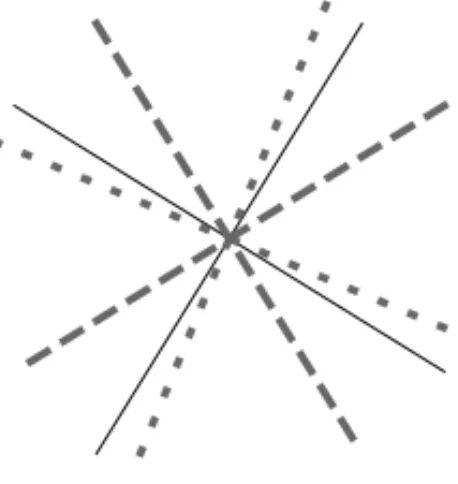
b1b2=2=0. The main directions of these matrices are displayed as dashed and dotted lines in Figure 1.
Figure 1: The directions of the columns of the minimizing matrixU(θ )in solid lines, and the main directions of the matricesM1andM2, in dashed and dotted lines. The matrices, given by Eq. (5.2), are not partially complementary and have different amplitudes.
In this case, according to Eqs. (4.11) and (4.12), the minimizing values ofθare given byθ = 1
4arctan( 4 3)−
π
4 +
qπ
0 Π 4
Π
2 0
1 2 3 4 5
Θ
f
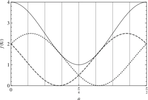
Figure 2: For the matrices of Figure 1, the objective functionF(U), in solid line, and the func-tions f(M1,U)e f(M2,U), in dashed and dotted lines.
5.2 Non partially complementary matrices of equal amplitudes
Now we consider the matrices
M1=
2 1
1 1
and M2=
1 1
1 2
, (5.3)
whose amplitudes equal 54. The matrices are not partially complementary, in fact, (a1 −c1) (a2−c2)+b1b2=3=0.
Figure 3: The directions of the columns of the minimizing matrixU(θ )in solid lines, and the main directions of the matricesM1andM2, in dashed and dotted lines. The matrices, given by Eq. (5.3), are not partially complementary and have equal amplitudes.
In this case, the minimizing angles areθ = π4 + q2π, whereq is an integer. In Figure 3, the solid lines given by such directions are bisectrices of the the smaller angles defined by the main directions ofM1andM2. This is clearly shown in Figure 4, where the objective functionsF(U),
0 Π 4
Π
2 0
1 2 3 4
Θ
f
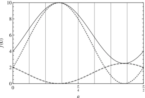
Figure 4: For the matrices of Figure 3, the objective functionF(U), in solid line, and the func-tions f(M1,U)e f(M2,U), in dashed and dotted lines.
5.3 Partially complementary matrices with different amplitudes
It is also interesting to consider the matrices
M1=
2 1
1 1
and M2=
2 1
1 6
, (5.4)
which have amplitudes 54 and 5. The matrices are partially complementary, since (a1−c1) (a2−c2)+b1b2=0. The anglesθ = −14arctan(43)+q2π, whereq is an integer, minimize the objective functionF(U).
Figure 5: The directions of the columns of the minimizing matrixU(θ )in solid lines, and the main directions of the matricesM1andM2, in dashed and dotted lines. The matrices, given by Eq. (5.4), are partially complementary and have different amplitudes.
In this case, as shown in Figure 5, the minimizing directions coincide with the main directions of the matrix having larger amplitude, namelyM2. Figure 6 displays the objective functionsF(U),
in complete out of phase, that is, the angles producing the maximum value for one matrix yield the minimum value for the other. Therefore, the term of larger amplitude is dominant in the sum
F(U).
0 Π
4
Π
2 0
2 4 6 8 10
Θ
f
Figure 6: For the matrices of Figure 5, the objective functionF(U), in solid line, and the func-tions f(M1,U)e f(M2,U), in dashed and dotted lines.
5.4 Fully complementary matrices
Finally, we consider the matrices
M1=
2 1
1 1
and M2=
1 12 1 2 3
, (5.5)
whose amplitudes equal 54. Since these matrices are partially complementary, that is,(a1−c1) (a2−c2)+b1b2=0, and have equal amplitudes, they are fully complementary.
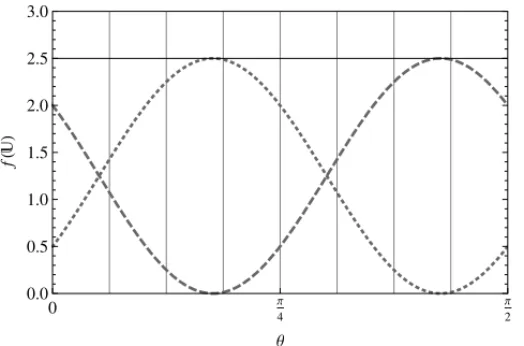
This is the case where the objective functionF(U)remains constant, as displayed in Figure 7. Therefore, one is not able to decrease the joint off-diagonal measure of the pair of matrices. Since no special value ofθ exist, a figure similar to Figures 1, 3 and 5 would not be meaningful in this case.
6 CONCLUSIONS
We have dealt with the problem of joint approximate diagonalization of a set of symmetric real matrices. The problem has been reduced to the search for the orthogonal transformation matrix that minimizes the joint off-diagonal sums of squares of the matrices.
0 Π 4
Π
2 0.0
0.5 1.0 1.5 2.0 2.5 3.0
Θ
f
Figure 7: The objective functionF(U), in solid line, and the functions f(M1,U)e f(M2,U), in dashed and dotted lines. The matrices, given by Eq. (5.5), are fully complementary.
other, we say that the matrices are partially complementary. Moreover, the sum of the squared off-diagonal entries of a transformed matrix oscillates harmonically, as a function of the rotation angle. The amplitude of the oscillation is one fourth of the squared difference between the eigen-values of the matrix. The results and discussions are presented for several cases, differing on whether the matrices are partially complementary and/or have equal amplitudes. The case where both situations apply deserves special attention because the joint approximate diagonalization has no effect, in other words, the objective function is constant. We say that such matrices are fully complementary.
We note that the joint approximate diagonalization is often applied to large matrices, and the numerical and computational aspects have been the main focus of precedent works. In contrast, our thorough discussion of matrices of order 2 has shed light on the geometrical meaning of the procedure. The introduction of the concepts of off-diagonalizing vectors, matrix amplitude and complementary matrices have been very useful and should find additional applications in Linear Algebra and other branches of science. Hopefully, the work will encourage the treatment of both complex and high-order matrices.
ACKNOWLEDGMENTS
The authors are grateful to the research group MApliC/Unesp for useful discussions.
RESUMO.Este trabalho aborda o problema da diagonalizac¸˜ao conjunta aproximada de uma colec¸˜ao de matrizes reais e sim´etricas. A otimizac¸˜ao ´e realizada com a restric¸ ˜ao de que a
ma-triz de transformac¸˜ao de semelhanc¸a seja ortogonal. As soluc¸˜oes s˜ao apresentadas de forma
anal´ıtica para matrizes de ordem 2. S˜ao introduzidos os conceitos de vetor anti-diagonalizan-te, amplitude de uma matriz, que ´e expressa em termos dos autovalores, e matrizes
conjunta aproximada, em termos dos autovetores e dos vetores anti-diagonalizantes das
matrizes. Esta contribuic¸˜ao deve auxiliar na melhoria de procedimentos num´ericos e com-putacionais envolvendo matrizes de ordem maior que 2.
Palavras-chave:diagonalizac¸˜ao conjunta aproximada, autovetores, otimizac¸˜ao.
REFERENCES
[1] Laurent Albera, Anne Ferr´eol, Pierre Comon & Pascal Chevalier. Blind Identification of Overcom-plete MixturEs of sources (BIOME).Linear Algebra and its Applications,391(2004), 3–30.
[2] Howard Anton & Chris Rorres.Elementary Linear Algebra – Applications Version, volume 10 (John Wiley & Sons, 2010).
[3] Adel Belouchrani, Karim Abed-Meraim, Jean-Franc¸ois Cardoso & Eric Moulines. A blind source separation technique using second-order statistics. Signal Processing, IEEE Transactions on 45(2) (1997), 434–444.
[4] Abdelwaheb Boudjellal, A. Mesloub, Karim Abed-Meraim & Adel Belouchrani. Separation of dependent autoregressive sources using joint matrix diagonalization. Signal Processing Letters, IEEE22(8) (2015), 1180–1183.
[5] Angelika Bunse-Gerstner, Ralph Byers & Volker Mehrmann. Numerical methods for simultaneous diagonalization.SIAM Journal on Matrix Analysis and Applications,14(4) (1993), 927–949.
[6] Augusto V. Cardona & Jos´e V.P. de Oliveira. Soluc¸˜aoE L T AN para o problema de transporte com
fonte.Trends in Applied and Computational Mathematics,10(2) (2009), 125–134.
[7] Augusto V. Cardona, R. Vasques & M.T. Vilhena. Uma nova vers˜ao do m´etodo L T AN.Trends in Applied and Computational Mathematics,5(1) (2004), 49–54.
[8] Jean-Franc¸ois Cardoso & Antoine Souloumiac. Jacobi angles for simultaneous diagonalization.
SIAM Journal on Matrix Analysis and Applications,17(1) (1996), 161–164.
[9] Gilles Chabriel, Martin Kleinsteuber, Eric Moreau, Hao Shen, Petr Tichavsk`y & Arie Yeredor. Joint matrices decompositions and blind source separation: A survey of methods, identification, and appli-cations.Signal Processing Magazine, IEEE,31(3) (2014), 34–43.
[10] Marco Congedo, Bijan Afsari, Alexandre Barachant & Maher Moakher, Approximate joint diagonal-ization and geometric mean of symmetric positive definite matrices.PloS one,10(4) (2015).
[11] Lieven De Lathauwer. A link between the canonical decomposition in multilinear algebra and simul-taneous matrix diagonalization.SIAM Journal on Matrix Analysis and Applications,28(3) (2006), 642–666.
[12] Klaus Glashoff and Michael M. Bronstein. Matrix commutators: their asymptotic metric properties and relation to approximate joint diagonalization.Linear Algebra and its Applications,439(8) (2013), 2503–2513.
[13] Franc¸ois Gygi, Jean-Luc Fattebert & Eric Schwegler. Computation of Maximally Localized Wan-nier Functions using a simultaneous diagonalization algorithm.Computer Physics Communications,
155(1) (2003), 1–6.
[15] Steven J. Leon.Linear Algebra with Applications, Eighth edition (Pearson, 2010).
[16] S.I. McNeill & D.C. Zimmerman. A framework for blind modal identification using joint approxi-mate diagonalization.Mechanical Systems and Signal Processing,22(7) (2008), 1526–1548.
[17] Anthony J. Pettofrezzo.Matrices and Transformations(Dover Publications, Inc., 1966).
[18] Dinh Tuan Pham. Joint approximate diagonalization of positive definite Hermitian matrices.SIAM Journal on Matrix Analysis and Applications,22(4) (2001), 1136–1152.
[19] Petr Tichavsk`y & Arie Yeredor. Fast approximate joint diagonalization incorporating weight matri-ces.Signal Processing, IEEE Transactions on57(3) (2009), 878–891.
[20] Roland Vollgraf & Klaus Obermayer. Quadratic optimization for simultaneous matrix diagonaliza-tion.IEEE Transactions on Signal Processing,54(9) (2006), 3270–3278.
[21] Arie Yeredor. Non-orthogonal joint diagonalization in the least-squares sense with application in blind