Pesqui. Oper. vol.33 número2

(1)

QAPV: A POLYNOMIAL INVARIANT FOR GRAPH ISOMORPHISM TESTING

Valdir Agustinho de Melo

1

, Paulo Oswaldo Boaventura-Netto

2*

and Laura Bahiense

3

Received September 21, 2011 / Accepted October 8, 2012

ABSTRACT.To each instance of the Quadratic Assignment Problem (QAP) a relaxed instance can be associated. Both variances of their solution values can be calculated in polynomial time. The graph isomor-phism problem (GIP) can be modeled as a QAP, associating its pair of data matrices with a pair of graphs of the same order and size. We look for invariant edge weight functions for the graphs composing the in-stances in order to try to find quantitative differences between variances that could be associated with the absence of isomorphism. This technique is sensitive enough to show the effect of a single edge exchange between two regular graphs of up to 3,000 vertices and 300,000 edges with degrees up to 200. Planar graph pairs from a dense family up to 300,000 vertices were also discriminated. We conjecture the existence of functions able to discriminate non-isomorphic pairs for every instance of the problem.

Keywords: graph isomorphism, quadratic assignment problem, variance.

1 INTRODUCTION

For each discussion presented in this work, the fundamental graph-theoretical concepts can be found in Harary [19] and Gross & Yellen [18]. A preliminary paper on the same subject, with abridged tests, is Meloet al.[26].

Thegraph isomorphism problemhas been studied by many researchers, owing to its theoretical interest and from its possible applications, such as pattern recognition, De Piero & Krout [10]. LetG1=(V1,E1)andG2=(V2,E2)be two simple graphs with independent labelings of their vertex sets. ThenG1andG2areisomorphicif and only if there is a bijectionϕ: V1 ↔V2that preserves their adjacency relations. Thegeneral problemarises whenG1is a graph andG2is a subgraph of another graph withat least the same ordernand sizemof G1. A particular case, which the present work addresses, is therestricted problem, which we will abbreviate asGIP.

*Corresponding author

1Program of Production Engineering, COPPE/UFRJ, Brazil. Post-doctoral researcher. E-mail: vmelo@pep.ufrj.br 2Universidade Federal do Rio de Janeiro/COPPE, Brazil. Full Professor, retired; Program of Production Engineering, COPPE/UFRJ. E-mail: boaventu@pep.ufrj.br

(2)

It is the problem of matching two graphs of the same order and size. It is is NP, but to date no one has been able to say if it is polynomial or NP-complete for every graph pair, Garey & Johnson [15], Arvind & Thoran [2].

The study of graph isomorphism has been done with the aid of two general classes of resources:

• matching algorithms, which look for building a graph in a way that matches an isomor-phism bijection, if it exists: McKay [27] proposed a specific one; Cross et al.[8] and Porumbel [29] use metaheuristics. DePiero & Krout [10] uses path counts to approximate subgraph isomorphism. Foggiaet al.[14] is a comparison among five commonly used al-gorithms. Goriet al.[16] use random walks. Jain & Wyzotski [22] uses neural nets; Ding & Huang [11] reorganize the graph in searching for a perimeter and a canonical adjacency matrix. Dharwadter & Tevet [13] presents a polynomial algorithm for the GIP, but Santos [31] found a counterexample for it. Presa [PR09] is a thesis on GIP algorithms. Czerwin-ski [9] is a theoretical paper which proposes a polynomial algorithm. Voss & Subhlock [34] is a performance comparison based on some graph classes, from 8 to 16,000 nodes. Douglas [12] discusses the possibility of applying the Weisfeiler-Lehman algorithm to the GIP, raising some open questions.

• efficient invariants. A graph parameter is (an)invariantif it has the same value for every isomorph of a given graph. The most readily available invariants are naturally the ordern and the sizem, but one would like to have an invariant where preserving value would be a necessary and sufficient condition for isomorphism – which is not, precisely, the case of order and size. An important invariant to consider is theordered degree set (ODS) associ-ated with a graph but, once again, two graphs with the same ODS can be non-isomorphic. On the other hand, two graphs withdifferent ODS arenon-isomorphic – and ODS is easy to calculate through a polynomial ordering algorithm. The graphspectrum(its set of adjacency matrix eigenvalues) is also an invariant but, again, there are non-isomorphic cospectralgraph pairs, Cvetkovicet al.[7]. Until now, necessary and sufficient invariance is an open research field, no invariant having been found which fulfills it. Most well-known invariants (such as the chromatic number and the independence number) are not polynomial, thus they are of no interest here.

This work proposes an invariant (the QAPV invariant) to be calculated using the Quadratic Assignment Problem (QAP)structure (Loiolaet al.[24]). Our aim is to translate into a non-zero deviation value anystructural differencebetween two graphs of the same order and size. If we obtain different values of this invariant for the two graphs, they will certainly be non-isomorphic: we say that we have been able todiscriminatebetween the two graphs. We present the results by giving agapbetween two values associated with the graphs.

(3)

meanings, a QAP instance can be constructed with the adjacency matrices of two simple graphs of equal order and size, which can be used to investigate isomorphism.

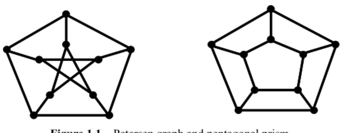
Despite the QAP’s NP-hardness, the calculation of the variance of a QAP instance’s solution set is polynomial, Boaventura-Netto & Abreu [4], Abreuet al.[1]. Given a graph pair (G,H), we can define two more instances, (G,G) and (H,H), and calculate these three variances. IfGandH are isomorphic, they have to be equal, but this is not sufficient for the graphs to be isomorphic: a counterexample is the pair (Petersen graph, pentagonal prism) in Figure 1.1.

Figure 1.1– Petersen graph and pentagonal prism.

To deal with this difficulty, we useinvariant edge weight functions: functions on the edge set whose values depend only on the graph structure and so are independent of the vertex numbering, thus reinforcing eventual differences between the graph structures. In this work, we present some such functions, discuss their complexity and apply them to sets of examples of regular and planar graphs and also to pairs obtained from public databases. The use of regular graphs has to do with the difficulty to be foreseen in discriminating between a given graph and another with closely similar structure: one could expect to find general non-regular graphs an easier problem to work with. Among the planar graphs, we chose the triangulated-grid family (6-point stencils, Voss & Subhlok [34], given by their order and rectangular(p,q)dimensions). Their square diagonals are built in the northeast-southwest direction, as in [34]. These graphs are near the maximum density for planar graphs; they haven= pq vertices andm=3n−2(p+q)+1 edges. Thus, a (600,500) graph of this type has almost 900,000 edges.

2 THEORETICAL BASIS

2.1 Quadratic Assignment Problem (QAP)

The QAP can be seen as the problem of how to assignnactivitieston positionsin such a way as to optimize the transportation cost between activity pairs over the distances associated with position pairs,

z∗= opt

ϕ∈5n X

1≤i<j≤n

fi jdϕ(i)ϕ(j) (2.1)

Minimization is the most frequent application, but when dealing with graph isomorphism we will be interested in maximization. MatrixF = [fi j]is theflow matrix(quantities transported

betweeni and j) and matrixD= [dkl]is thedistance matrix, wheredklis the distance between

(4)

The parcels of (2.1) are related to the set5n of alln-element permutations, with every QAP

solution being associated with a permutation ϕ ∈ 5n, in this case, based on positions with respect to activities. Thus, QAP structure is evidently attractive when examining the restricted GIP: if G1and G2are isomorphic with adjacency matricesA1andA2, we will find in the solution set of QAP(A1,A2) a permutation corresponding to their isomorphism relation. We give further attention to this point in Item 2.3.

Since graph isomorphism preserves the adjacency relations, if we look for amaximumvaluez∗ of a solution for such an instance we will find either z∗ = m, if the graphs are isomorphic, or z∗_<_{m, if they are not. The first result is a necessary and sufficient condition for isomorphism,}

but we immediately run into a complexity problem: the QAP is NP-hard and experience shows its exact resolution is presently limited, with some exceptions, to instances with order below 40. Specially designed heuristics, as well as metaheuristics, have been applied to it. With these resources, graph pairs of higher order have been successfully tested for isomorphism by treating them as QAP instances, Leeet al. [25], the results being subjected to the error margin of the heuristics.

2.2 Statistic moments of QAP instances

Average solution value and variance of solution values have been used to compare the computa-tional difficulty of QAP instances with respect to heuristic algorithms. We will be concerned with the results of Graves & Whinston, [17] and Abreuet al.[1]. Let us discuss briefly the calculation presented there.

We can store the data of a symmetric QAP instance with the aid of two vectors,FandD, with orderN =n(n−1)/2, respectively associated with the matricesFandD, where a vector position kcan be associated with a matrix position(i,j)by the expression

k=(i−1)n−i(i+1)/2+ j. (2.2)

We can then define aN-order matrix,Q=FDT, which contains every parcel composing every QAP solutionϕ (n-order permutation). Since (2.1) shows us both i and j(i < j)with values between 1 andn, every QAP solution has N parcels, which correspond to a set of independent positions inQ. Alln!solutions of a given instance can be found there among the wholeN!sets of this type. A problem based on Qis therefore a relaxationof the original QAP, where not every set of independent positions corresponds to a feasible QAP solution. We will denote such relaxation as Q A P(Q). We have also use for ordered vectorsF−andD+obtained fromFand Dthrough non-decreasing and non-increasing orderings respectively, from which we define a matrixQ′=(F−)(D+)T.

Let S be the sum of allQelements. Then the average cost of an instanceQ A P(F,D), [1], [3], [4], [17], is

(5)

The variance of the relaxed instance,Q A P(Q), is, [1], [17],

σ_Q2 = 1 N

N

X

i=1 f₁2

N

X

i=1 d2_j

+ 1

N(N−1)

σ2(fi)σ2(dj)−μ2(i,j =1, . . . ,n) (2.4)

The variance of the (original) instanceQ A P(F,D)is, [1], [4],

σ_F,D2 = S0+S1+S2n! −μ2, (2.5)

where

S0 = 4(n−4)!

X

∩0 fi j fr s

X

∩0

di jdr s (2.6)

S1 = (n−3)!

X

∩1 fi jfr s

X

∩1

di jdr s (2.7)

S2 = 2(n−2)!

X

1≤i<j≤n

fi j2 X

1≤i<j≤n

di j2 (2.8)

and

| ∩0| =Cn−2,2,| ∩1| =2(n−2) (2.9) where∩k(k∈ {0,1})is the set of pairs((i,j), (r,s))such that|{i,j} ∩ {r,s}| =k.

The computational complexity of the first variance is thusO(n2), and that of the second isO(n4), in both cases, consideringFandDas full matrices. By using adjacency lists, they becomeO(m)

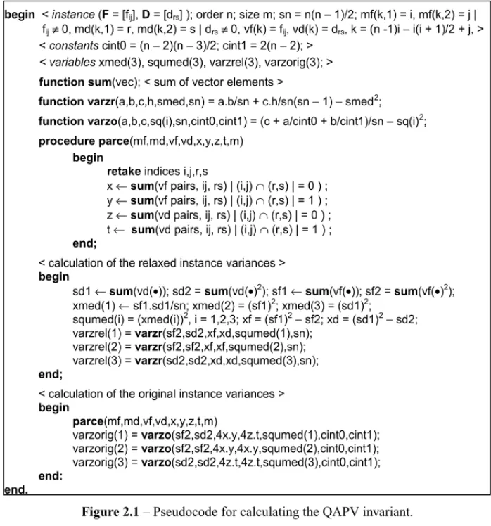
andO(m2₎_{respectively. The reuse of several terms gives way to a significant time economy,} as shown by the pseudocode below, which includes the three-instance calculation referred to in Item 1 (Figure 2.1):

2.3 Instance classes related to isomorphism

We can define a Q A P(F−,D+)with coefficient matrixQ′ and then define a related instance class where the ordering of every pair(F,D)will result in the sameQ′, [1],

Relclass(F−,D+)=

Q A P(F,D)/(F−)(D+)T =Q′ (2.10)

By going into graph language, a QAP instance can be represented by two complete graphsKF

andKD, respectively edge-valued by the weight functionsw(KF)=Fandw(KD)=D.

We will then say that two edge-valued complete graphsKn(V1,E1,F)andKn(V2,E2,D)are

(6)

< ( = [fij], = [drs] ); order n; size m; sn = n(n – 1)/2; mf(k,1) = i, mf(k,2) = j | fij≠_{0, md(k,1) = r, md(k,2) = s | drs}≠_{0, vf(k) = fij, vd(k) = drs, k = (n -1)i – i(i + 1)/2 + j, >}

< cint0 = (n – 2)(n – 3)/2; cint1 = 2(n – 2); > xmed(3), squmed(3), varzrel(3), varzorig(3); >

(vec); < sum of vector elements >

(a,b,c,h,smed,sn) = a.b/sn + c.h/sn(sn – 1) – smed2; (a,b,c,sq(i),sn,cint0,cint1) = (c + a/cint0 + b/cint1)/sn – sq(i)2_;

(mf,md,vf,vd,x,y,z,t,m)

indices i,j,r,s

x ← _{(vf pairs, ij, rs) | (i,j)}∩_{(r,s) | = 0 ) ;}

y ← (vf pairs, ij, rs) | (i,j) ∩ (r,s) | = 1 ) ;

z ← _{(vd pairs, ij, rs) | (i,j)}∩_{(r,s) | = 0 ) ;}

t ← (vd pairs, ij, rs) | (i,j) ∩ (r,s) | = 1 ) ;

< calculation of the relaxed instance variances >

sd1 ← _(vd(•_{)); sd2 =} _(vd(•₎2_{); sf1}← _(vf(•_{)); sf2 =} _(vf(•₎2_);

xmed(1) ←_{sf1.sd1/sn; xmed(2) = (sf1)}2_{; xmed(3) = (sd1)}2_;

squmed(i) = (xmed(i))2, i = 1,2,3; xf = (sf1)2 – sf2; xd = (sd1)2 – sd2; varzrel(1) = (sf2,sd2,xf,xd,squmed(1),sn);

varzrel(2) = (sf2,sf2,xf,xf,squmed(2),sn); varzrel(3) = (sd2,sd2,xd,xd,squmed(3),sn);

< calculation of the original instance variances >

(mf,md,vf,vd,x,y,z,t,m)

varzorig(1) = (sf2,sd2,4x.y,4z.t,squmed(1),cint0,cint1); varzorig(2) = (sf2,sf2,4x.y,4x.y,squmed(2),cint0,cint1); varzorig(3) = (sd2,sd2,4z.t,4z.t,squmed(3),cint0,cint1);

Figure 2.1– Pseudocode for calculating the QAPV invariant.

On the other hand, we say thatG1=(V1,E1)andG2=(V2,E2)are isomorphic if and only if there exists a function f which preserves the adjacency relations over a permutationαof one of their vertex sets with respect to the other, that is, for every(i,j)∈E1we have f(α(i), α(j))∈

E2.

This isomorphism appears then as a particular case of the w-isomorphism defined in the context of QAP, where the weight function is given by the adjacency matrix for a graphG = (V,E), A= [ai j],ai j =1 if(i,j)∈E and ai j =0 if (i,j) /∈E.

The theorem and corollary below constitute the basis for the application of QAP variance on GIP.

Theorem 2.1[1]: Two isomorphic instances Q A P(F1,D1)and Q A P(F2,D2)have the same set of feasible solutions.

(7)

Corollary 2.2.Two isomorphic instances have the same variance.

Proof.Immediate from Theorem 2.1, since they share the same set of feasible solutions.

The variance of QAP solutions is then an invariant with respect to instance isomorphism. In Section 1, we had an initial look at the practical use of this property, but it requires a more detailed discussion.

Trying to avoid variance equality when using the comparison sketched in Section 1 with non-isomorphic graphs (such as those in Figure 1.1), we propose to giveweightsto the edges, thus obtaining matrices which could be tested forw-isomorphism. For this to have a meaning, these values have to be given by aninvariant function– that is, a function whose values correspond to a property of the graphstructure– which is given by its adjacency relations, preserved by isomorphism and not related to vertex labeling.

3 METHODOLOGY

3.1 A comparison standard and the use of weight functions

Let us callQ A P(G1,G2)the instance built with the adjacency matrices of two graphs. We then associate two other instances with it,Q A P(G1,G1)andQ A P(G2,G2)with two copies of the same matrix for each graph. We will call these last two instances associated instances, and their variances, associated variances. Both for the original and the relaxed instances, Corollary 2.2 is only anecessarycondition: to have the same variance is not sufficient for two instances to be isomorphic. A consequence of this is that a number of graph pairs with approximately similar structures show equal variances for the three instances presented above.

We try to overcome this difficulty by applyingedge invariant weight functions, going intow -isomorphism to look for discrimination between the graphs of such pairs. In this work, we use the following functions, whose complexity is presented considering the use of adjacency lists. We will represent them as f(G), where it is understood that the function concerns the edge set E, forG=(V,E).

• Functionw3(G): number of 3-edge closed walksusing the concerned edge: this function can be calculated in O(nd).

• Function w4(G): number of 4-edge closed walks using the concerned edge: it is more costly since it deals with a larger neighborhood. The worst complexity case is O(n2d).

These two functions can be calculated with the aid of the following theorem, the second one being obtained from the first one by induction:

Theorem 3.1(Festinger,apudBoaventura-Netto [5]). Let G =(V,E)be a graph,A= [ai j]

(8)

Since we are interested in valuating pairsi,j which define edges, the exponent to be used will be the length of the walks minus one (k = 2 or 3 respectively to calculatew3(G)andw4(G)). Other similar functions can be used, according to the girth of the graphs examined, but the complexity grows rapidly. We can also define new functions by summing the obtained values into the adjacency matrix, which can be beneficial with sparse graphs, thus making graph extensions in the sense of Porumbel [29].

• Functiondc(G): dcstands fordistance to centers: it can be calculated with all-distances techniques such as Floyd orn-times applied Dijkstra algorithms. We use the distance matrix to find the graph center setCand then, for everyv ∈ V, we calculatedc(v) =

P ˉ

c∈Cd(v,c). The function value for the edge (i,j)is given by the sum of the values

obtained foriand j. The initial “infinite” values of non-existing edges will be greater than n. The complexity depends on the implementation, going from O(n2logn)to O(n3).

• Functiones(G):esstands foredge sum: for each vertex, it is the sum of its adjacent edge values. The edge function value is then the value sum of its adjacent vertices.es(G)should not be directly applied to regular graphs (it would give equal values for all edges) but it can be applied to a regular graph already valued with the aid of another function, for example, es(w3(G)). The complexity is O(m).

Other functions can be devised as discriminating tools, provided they are invariant and poly-nomial, as in Bessaet al.[6].

3.2 Graph families used in the tests

We used a regular graph generator where the vertex pair selection for edge introduction was randomly done with the aid of two random number generators, a conventional product-overflow generator and, for larger graphs, a (5,17) lagged-Fibonacci generator, Marsaglia [28], Knuth [23]. The program contains an edge reallocation routine designed to correct regularity failures which are intrinsic to direct generation. Ten graphs of each order and degree were created this way.

We also generated what we callalmost-isomorphicgraphs by making random2-exchangesin each original graph in order to create structural differences. We define a2-exchangeas an edge exchange inG = (V,E)where we take off two edges (a,b), (c,d) ∈E and replace them with either (a,c), (b,d)∈/E, or (a,d), (b,c)∈/E, thus preserving ODS. For each chosen(n,d)pair, we constructed ten sets composed of an original graph and two almost isomorphs of it, comprising one graph with one 2-exchange and another with four 2-exchanges. We applied the weight func-tions to all these graphs. The data set has regular graphs with orders 50, 100, 200, 500, 1000, 1500, 2000, 2500 and 3000, withd ≤n/2 andd ∈ {3,5,10,25,50,100,200}. Higher degree values were not used to generate the bigger graphs, in order to limit to acceptable values the processing times required by the weight functions.

(9)

we eliminated the northeast upper diagonal. The corresponding squares formed what we called windows in the graph, creating localized structure differences among them. To the graphs thus obtained we applied the functiones2(G) and we took them two by two to build ten QAP instances. Order values and rectangle dimensions were 4,000 (50,80), 5,000 (50,100), 7,000 (70,100), 10,000 (100,100), 15,000 (150,100), 20,000 (200,100), 30,000 (200,150), 40,000 (200,200), 50,000 (250,200), 60,000 (300,200), 80,000 (400,200), 100,000 (400,250), 150,000 (500,300), 200,000 (500,400), 250,000 (500,500) and 300,000 (600,500). All used databases can be found in [5].

3.3 Discrimination measure

The discrimination instrument was the total percentage gap between the variance relation of the associated instances,σ2[Q A P(f(G1),f(G1))]andσ2[Q A P(f(G2),f(G2))], and that of the instance built with the graph pair,σ2(Q A P(f(G1),f(G2)), calculated up to 10−12,

R%G1 = 100σ2[Q A P(f(G1),f(G1))]σ2[Q A P(f(G1),f(G2))] (3.1)

R%G2 = 100σ2[Q A P(f(G2),f(G2))]σ2[Q A P(f(G1),f(G2))] (3.2)

Gap(G1,G2) = |R%G1| + |R%G2|. (3.3)

From the previous discussion, apositive gap indicates absence of isomorphism while a null gap fails to discriminate between the pair of graphs. The results involve both the original and the relaxed instances. We know thatRelclass(F−,D+)includes non-isomorphic graphs, then it can happen that the relaxed instances calculation do not show discrimination. However, if we obtain this discrimination, it would be sufficient to guarantee the absence of isomorphism with a much lower computational cost. Most of our examples show this behavior, which can be seen in Tables 4.1 (a) and (b), where we list the number of discriminations out of each set of ten graphs.

4 COMPUTATIONAL RESULTS

4.1 Discrimination results for regular graphs

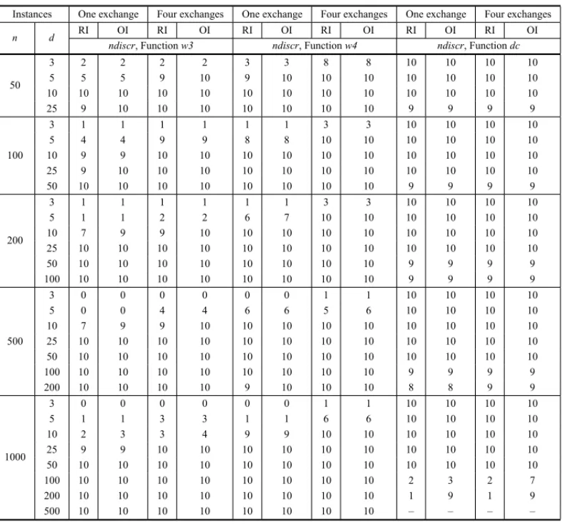
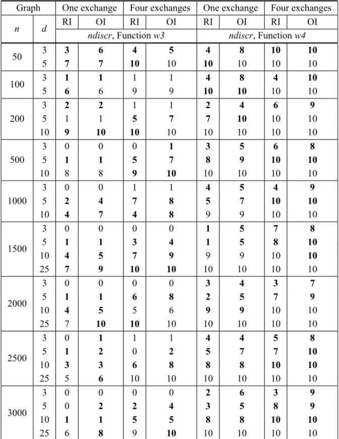
Tables 4.1 (a) and (b) show the results obtained with functionsw3,w4 anddcfor the regular 10-graph sets with given(n,d)values. Columnsndi scr show the number of instances (out of 10) where discrimination was obtained. Results are given for relaxed (RI)and original (OI)

instances, with 1 and 4 random 2-exchanges.

(10)

Table 4.1(a)– Discrimination results of QAPV invariant on almost-isomorphic regular graph pairs.

Instances One exchange Four exchanges One exchange Four exchanges One exchange Four exchanges

n d RI OI RI OI RI OI RI OI RI OI RI OI

ndiscr, Functionw3 ndiscr, Functionw4 ndiscr, Functiondc

50

3 2 2 2 2 3 3 8 8 10 10 10 10

5 5 5 9 10 9 10 10 10 10 10 10 10

10 10 10 10 10 10 10 10 10 10 10 10 10

25 9 10 10 10 10 10 10 10 9 9 9 9

3 1 1 1 1 1 1 3 3 10 10 10 10

5 4 4 9 9 8 8 10 10 10 10 10 10

100 10 9 9 10 10 10 10 10 10 10 10 10 10

25 9 10 10 10 10 10 10 10 10 10 10 10

50 10 10 10 10 10 10 10 10 9 9 9 9

200

3 1 1 1 1 1 1 3 3 10 10 10 10

5 1 1 2 2 6 7 10 10 10 10 10 10

10 7 9 9 10 10 10 10 10 10 10 10 10

25 10 10 10 10 10 10 10 10 10 10 10 10

50 10 10 10 10 10 10 10 10 9 9 9 9

100 10 10 10 10 10 10 10 10 9 9 9 9

3 0 0 0 0 0 0 1 1 10 10 10 10

5 0 0 4 4 6 6 5 6 10 10 10 10

10 7 9 9 10 10 10 10 10 10 10 10 10

500 25 10 10 10 10 10 10 10 10 10 10 10 10

50 10 10 10 10 10 10 10 10 10 10 10 10

100 10 10 10 10 10 10 10 10 9 9 9 9

200 10 10 10 10 9 10 10 10 8 8 9 9

1000

3 0 0 0 0 0 0 1 1 10 10 10 10

5 1 1 3 3 1 1 6 6 10 10 10 10

10 2 3 3 4 9 9 10 10 10 10 10 10

25 9 9 10 10 10 10 10 10 10 10 10 10

50 10 10 10 10 10 10 10 10 10 10 10 10

100 10 10 10 10 10 10 10 10 2 3 2 7

200 10 10 10 10 10 10 10 10 1 9 1 9

500 10 10 10 10 10 10 10 10 – – – –

Functiondc(G)was 100% efficient with all instance sets of lower degree, thus complementing the range of the other two functions. We can see that it does not perform as well with the denser graphs, owing probably to the equalization of the number of centers and to lesser distance ranges. The results from the (1000,100) and (1000,200) pairs, for instance, were not good and that led us to abandon the idea of testing higher degrees.

We can also observe that, in most cases, a single 2-exchange was enough for the invariant to show a structural difference, specially with functiondc(G).

Finally, we exemplify the application ofes(w3(G))andes(w4(G))by using it with lesser-degree instances, where w3(G), and even w4(G), encountered difficulties in discriminating between pairs of almost isomorphs. Table 4.2 shows these results, which can be compared with those from Tables 4.1 (a) and (b) for the same instance collections.

(11)

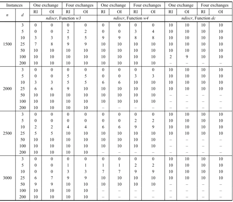
Table 4.1(b)– Discrimination results of QAPV invariant on almost-isomorphic regular graph pairs.

Instances One exchange Four exchanges One exchange Four exchanges One exchange Four exchanges

n d RI OI RI OI RI OI RI OI RI OI RI OI

ndiscr, Functionw3 ndiscr, Functionw4 ndiscr, Functiondc

3 0 0 0 0 0 0 0 0 10 10 10 10

5 0 0 2 2 0 0 3 4 10 10 10 10

10 3 3 5 5 9 9 8 8 10 10 10 10

1500 25 7 8 9 9 10 10 10 10 10 10 10 10

50 10 10 10 10 10 10 10 10 10 10 10 10

100 10 10 10 10 10 10 10 10 2 9 10 10

200 10 10 10 10 10 10 10 10 – – – –

3 0 0 0 0 0 0 0 0 10 10 10 10

5 0 0 5 5 0 0 3 3 10 10 10 10

10 3 3 5 5 6 6 10 10 10 10 10 10

2000 25 6 6 9 10 10 10 10 10 10 10 10 10

50 10 10 10 10 10 10 10 10 – – – –

100 10 10 10 10 10 10 10 10 – – – –

200 10 10 10 10 – – – – – – – –

3 0 0 0 0 0 0 0 0 10 10 10 10

5 0 0 0 0 0 0 2 2 10 10 10 10

10 2 2 4 4 6 6 9 9 10 10 10 10

2500 25 5 5 10 10 10 10 10 10 10 10 10 10

50 10 10 10 10 10 10 10 10 – – – –

100 10 10 10 10 10 10 10 10 – – – –

200 10 10 10 10 – – – – – – – –

3 0 0 0 0 0 0 0 0 10 10 10 10

5 0 0 1 1 1 1 2 2 10 10 10 10

10 0 0 3 3 7 7 9 9 10 10 10 10

3000 25 6 7 9 9 10 10 10 10 10 10 10 10

50 9 9 10 10 10 10 10 10 – – – –

100 10 10 10 10 – – – – – – – –

200 10 10 10 10 – – – – – – – –

constitute a significant majority of those values that can be enhanced (discr < 10), (see, for instance, the 25-regular graphs withw4(G),n ≥ 1500, compared with those of Table 4.1(b)). In the whole, this experiment shows about 78% of enhanced values, which is interesting because of the very low cost of this function. For some instances, this application is fruitless; some ex-amples are the 3-regular graphs with 1000 or more vertices. We think that, in these cases, the structures associated withw3(G)andw4(G)(3- and 4-closed walks) do not easily exist in the graphs, a situation which can be found in large, low-degree regular graphs, where larger girths are to be expected.

4.2 Processing times for regular graphs

(12)

Table 4.2– Application ofes(f(G))to some instance collections affected byw3(G)andw4(G).

Graph One exchange Four exchanges One exchange Four exchanges

n d RI OI RI OI RI OI RI OI

ndiscr, Functionw3 ndiscr, Functionw4

50 3 3 6 4 5 4 8 10 10

5 7 7 10 10 10 10 10 10

100 3 1 1 1 1 4 8 4 10

5 6 6 9 9 10 10 10 10

3 2 2 1 1 2 4 6 9

200 5 1 1 5 7 7 10 10 10

10 9 10 10 10 10 10 10 10

3 0 0 0 1 3 5 6 8

500 5 1 1 5 7 8 9 10 10

10 8 8 9 10 10 10 10 10

3 0 0 1 1 4 5 4 9

1000 5 2 4 7 8 5 7 10 10

10 4 7 4 8 9 9 10 10

1500

3 0 0 0 0 1 5 7 8

5 1 1 3 4 1 5 8 10

10 4 5 7 9 9 9 10 10

25 7 9 10 10 10 10 10 10

2000

3 0 0 0 0 3 4 3 7

5 1 1 6 8 2 5 7 9

10 4 5 5 6 9 9 10 10

25 7 10 10 10 10 10 10 10

2500

3 0 1 1 1 4 4 5 8

5 1 2 0 2 5 7 7 10

10 3 3 6 8 8 8 10 10

25 5 6 10 10 10 10 10 10

3000

3 0 0 0 0 2 6 3 9

5 0 2 2 4 3 5 8 9

10 1 1 5 5 8 8 10 10

25 6 8 9 10 10 10 10 10

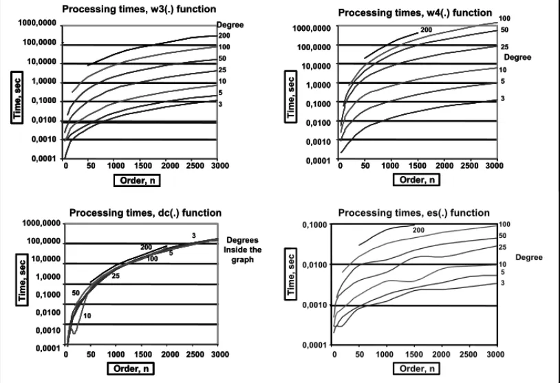
We can see that the processing time for es(.) is negligible when compared with the other functions.

By examining Figures 4.1 and 4.2, we see that the graphs show comparable times betweenw3(G) and variance calculation, withw4(G)taking more time. The times depend on the graph degree with the exception ofdc(G), whose time requirements are almost constant for a given order.

4.3 Going to practical application

(13)

Figure 4.1– Processing times for weight functions applied to regular graphs.

Figure 4.2– Processing times of QAPV invariant for regular QAP-GIP instances.

Conjecture 4.1. For every graph pair (G1,G2)of the same order and size, there exists a polynomial invariant weight function such that, for non-isomorphic G1and G2, the instances Q A P(G1,G2), Q A P(G1,G1)and Q A P(G2,G2)will have different variances.

(14)

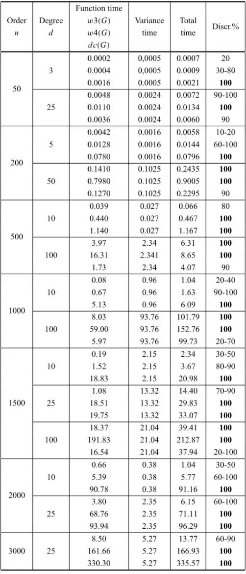
Table 4.3– Discrimination and total QAPV processing time for some regular graph instances.

Function time

Discr.%

Order Degree w3(G) Variance Total

n d w4(G) time time

dc(G)

50

0.0002 0,0005 0.0007 20

3 0.0004 0,0005 0.0009 30-80

0.0016 0.0005 0.0021 100

0.0048 0.0024 0.0072 90-100

25 0.0110 0.0024 0.0134 100

0.0036 0.0024 0.0060 90

200

0.0042 0.0016 0.0058 10-20

5 0.0128 0.0016 0.0144 60-100

0.0780 0.0016 0.0796 100

0.1410 0.1025 0.2435 100

50 0.7980 0.1025 0.9005 100

0.1270 0.1025 0.2295 90

500

0.039 0.027 0.066 80

10 0.440 0.027 0.467 100

1.140 0.027 1.167 100

3.97 2.34 6.31 100

100 16.31 2.341 8.65 100

1.73 2.34 4.07 90

1000

0.08 0.96 1.04 20-40

10 0.67 0.96 1.63 90-100

5.13 0.96 6.09 100

8.03 93.76 101.79 100

100 59.00 93.76 152.76 100

5.97 93.76 99.73 20-70

1500

0.19 2.15 2.34 30-50

10 1.52 2.15 3.67 80-90

18.83 2.15 20.98 100

1.08 13.32 14.40 70-90

25 18.51 13.32 29.83 100

19.75 13.32 33.07 100

18.37 21.04 39.41 100

100 191.83 21.04 212.87 100

16.54 21.04 37.94 20-100

2000

0.66 0.38 1.04 30-50

10 5.39 0.38 5.77 60-100

90.78 0.38 91.16 100

3.80 2.35 6.15 60-100

25 68.76 2.35 71.11 100

93.94 2.35 96.29 100

8.50 5.27 13.77 60-90

3000 25 161.66 5.27 166.93 100

(15)

5 TESTS WITH TRIANGULATED-GRID GRAPHS

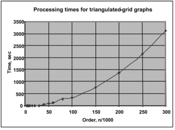
The almost-isomorphs used in the tests allowed 100% discrimination with the (50,80), (50,100), (70,100), (100,100), (150,100), (200,100), (200,200) and (500,500) instances. The (200,150), (250,200), (300,200), (400,200), (400,250), (500,300) and (500,400) instances had 90% discrim-ination. The (600,500) instance testes showed 70% discrimdiscrim-ination. Discrimination was always the same with relaxed and original instances. For each of these tests, five almost-isomorphs were randomly generated and compared two by two, thus allowing ten comparisons.

The processing time of all relaxed instances was negligible (≤0.002 sec). Figure 5.1 shows the processing time for the original instances.

Figure 5.1– Processing times of QAPV for TGG.

As an example, Figure 5.2 shows a (15,11)-TGG with four windows (indicated by the circles).

(16)

6 AN EXAMPLE OF ISOMORPHISM

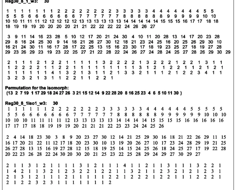
As a case of isomorphism, we present a (30,8) graph and an isomorph of it characterized by a given permutation, applyingw3(G)to both of them. The graphs are described by their non-symmetric valued adjacency lists, firstlyvi ∈ V, thenvj|∃(vi, vj),j >i and finally, the

corre-spondingw3(G)edge values. The main instance and its associates produced the same variance values (R% null), both with the relaxed and with the original instances (Fig. 6.1):

Reg30_8_1_w3: 30

1 1 1 1 1 1 1 2 2 2 2 2 2 2 2 3 3 3 3 3 4 4 4 4 4 4 4 5 5 5 5 5 6 6 6 6 6 6 6 7 7 7 7 7 7 8 8 8 8 8 8 9 9 9 9 9 10 10 10 10 11 11 11 12 12 12 12 12 13 13 13 13 13 13 14 14 14 14 14 15 15 15 16 17 17 18 18 18 19 19 19 20 20 20 20 21 21 22 22 22 22 24 26 26 27

3 9 11 14 16 23 28 5 10 12 17 20 21 24 30 4 10 11 20 28 13 14 17 20 23 28 29 8 16 24 25 30 9 14 18 21 26 27 30 12 18 21 23 24 25 16 20 25 26 29 30 10 16 21 24 30 11 16 17 28 17 22 25 13 15 16 23 30 17 18 19 23 25 27 18 19 27 28 29 23 26 29 23 19 23 22 25 27 21 22 28 22 24 26 27 24 28 24 25 27 28 26 29 30 29

2 1 1 1 2 1 2 2 1 1 1 1 1 3 2 2 2 2 1 3 2 2 2 1 2 2 1 3 1 1 1 2 2 2 2 1 1 2 2 1 1 1 1 1 1 1 1 1 3 1 2 1 2 2 1 1 2 1 2 1 1 1 1 1 1 1 4 1 3 2 1 3 1 1 2 1 3 3 2 1 1 1 2 1 2 2 3 4 1 1 3 2 3 2 1 3 1 1 2 2 1 1 2 2 1

Permutation for the isomorph:

(13 2 7 19 1 17 29 18 24 27 26 3 21 15 12 14 9 22 28 20 8 16 25 23 4 6 5 10 11 30 )

Reg30_8_1iso1_w3: 30

1 1 1 1 1 1 2 2 2 2 2 2 2 3 3 3 3 3 3 4 4 4 4 4 4 5 5 5 5 5 5 5 6 6 6 6 6 6 6 7 7 7 7 7 7 8 8 8 8 8 8 9 9 9 9 9 9 10 10 10 10 10 10 11 11 11 11 12 13 13 13 13 13 14 14 14 14 15 15 15 15 16 16 16 16 16 17 17 17 18 18 19 19 19 20 21 21 21 22 23 23 24 24 25 26

2 4 14 18 23 30 3 8 9 20 23 27 30 12 14 21 25 29 30 16 18 21 22 26 29 11 15 16 17 20 21 22 11 12 17 18 20 23 30 10 13 19 20 26 27 10 17 23 24 28 29 19 21 25 26 27 28 13 15 16 19 27 28 12 15 18 19 25 14 15 24 25 26 18 24 25 27 17 19 22 28 20 22 23 26 28 22 24 30 20 30 20 21 25 23 22 25 28 29 24 29 27 30 29 27

2 1 1 3 1 2 1 1 1 1 3 1 2 1 1 1 4 1 1 2 1 1 3 1 1 1 3 2 2 1 1 4 2 1 1 3 2 1 2 3 2 2 1 2 2 1 1 3 2 1 1 2 3 2 1 2 1 2 3 1 2 1 3 1 2 1 1 1 2 1 1 1 1 1 2 2 1 2 2 2 1 2 2 1 1 1 2 2 2 1 2 1 2 2 3 2 3 1 1 1 1 1 1 1 2

Variances for the three test instances: relaxed 170.1935335, originals 173.3623220. Gaps null.

Reg30_8_1_w3: 30

1 1 1 1 1 1 1 2 2 2 2 2 2 2 2 3 3 3 3 3 4 4 4 4 4 4 4 5 5 5 5 5 6 6 6 6 6 6 6 7 7 7 7 7 7 8 8 8 8 8 8 9 9 9 9 9 10 10 10 10 11 11 11 12 12 12 12 12 13 13 13 13 13 13 14 14 14 14 14 15 15 15 16 17 17 18 18 18 19 19 19 20 20 20 20 21 21 22 22 22 22 24 26 26 27

3 9 11 14 16 23 28 5 10 12 17 20 21 24 30 4 10 11 20 28 13 14 17 20 23 28 29 8 16 24 25 30 9 14 18 21 26 27 30 12 18 21 23 24 25 16 20 25 26 29 30 10 16 21 24 30 11 16 17 28 17 22 25 13 15 16 23 30 17 18 19 23 25 27 18 19 27 28 29 23 26 29 23 19 23 22 25 27 21 22 28 22 24 26 27 24 28 24 25 27 28 26 29 30 29

2 1 1 1 2 1 2 2 1 1 1 1 1 3 2 2 2 2 1 3 2 2 2 1 2 2 1 3 1 1 1 2 2 2 2 1 1 2 2 1 1 1 1 1 1 1 1 1 3 1 2 1 2 2 1 1 2 1 2 1 1 1 1 1 1 1 4 1 3 2 1 3 1 1 2 1 3 3 2 1 1 1 2 1 2 2 3 4 1 1 3 2 3 2 1 3 1 1 2 2 1 1 2 2 1

(13 2 7 19 1 17 29 18 24 27 26 3 21 15 12 14 9 22 28 20 8 16 25 23 4 6 5 10 11 30 )

Reg30_8_1iso1_w3: 30

1 1 1 1 1 1 2 2 2 2 2 2 2 3 3 3 3 3 3 4 4 4 4 4 4 5 5 5 5 5 5 5 6 6 6 6 6 6 6 7 7 7 7 7 7 8 8 8 8 8 8 9 9 9 9 9 9 10 10 10 10 10 10 11 11 11 11 12 13 13 13 13 13 14 14 14 14 15 15 15 15 16 16 16 16 16 17 17 17 18 18 19 19 19 20 21 21 21 22 23 23 24 24 25 26

2 4 14 18 23 30 3 8 9 20 23 27 30 12 14 21 25 29 30 16 18 21 22 26 29 11 15 16 17 20 21 22 11 12 17 18 20 23 30 10 13 19 20 26 27 10 17 23 24 28 29 19 21 25 26 27 28 13 15 16 19 27 28 12 15 18 19 25 14 15 24 25 26 18 24 25 27 17 19 22 28 20 22 23 26 28 22 24 30 20 30 20 21 25 23 22 25 28 29 24 29 27 30 29 27

2 1 1 3 1 2 1 1 1 1 3 1 2 1 1 1 4 1 1 2 1 1 3 1 1 1 3 2 2 1 1 4 2 1 1 3 2 1 2 3 2 2 1 2 2 1 1 3 2 1 1 2 3 2 1 2 1 2 3 1 2 1 3 1 2 1 1 1 2 1 1 1 1 1 2 2 1 2 2 2 1 2 2 1 1 1 2 2 2 1 2 1 2 2 3 2 3 1 1 1 1 1 1 1 2

Reg30_8_1_w3: 30

1 1 1 1 1 1 1 2 2 2 2 2 2 2 2 3 3 3 3 3 4 4 4 4 4 4 4 5 5 5 5 5 6 6 6 6 6 6 6 7 7 7 7 7 7 8 8 8 8 8 8 9 9 9 9 9 10 10 10 10 11 11 11 12 12 12 12 12 13 13 13 13 13 13 14 14 14 14 14 15 15 15 16 17 17 18 18 18 19 19 19 20 20 20 20 21 21 22 22 22 22 24 26 26 27

3 9 11 14 16 23 28 5 10 12 17 20 21 24 30 4 10 11 20 28 13 14 17 20 23 28 29 8 16 24 25 30 9 14 18 21 26 27 30 12 18 21 23 24 25 16 20 25 26 29 30 10 16 21 24 30 11 16 17 28 17 22 25 13 15 16 23 30 17 18 19 23 25 27 18 19 27 28 29 23 26 29 23 19 23 22 25 27 21 22 28 22 24 26 27 24 28 24 25 27 28 26 29 30 29

2 1 1 1 2 1 2 2 1 1 1 1 1 3 2 2 2 2 1 3 2 2 2 1 2 2 1 3 1 1 1 2 2 2 2 1 1 2 2 1 1 1 1 1 1 1 1 1 3 1 2 1 2 2 1 1 2 1 2 1 1 1 1 1 1 1 4 1 3 2 1 3 1 1 2 1 3 3 2 1 1 1 2 1 2 2 3 4 1 1 3 2 3 2 1 3 1 1 2 2 1 1 2 2 1

(13 2 7 19 1 17 29 18 24 27 26 3 21 15 12 14 9 22 28 20 8 16 25 23 4 6 5 10 11 30 )

Reg30_8_1iso1_w3: 30

1 1 1 1 1 1 2 2 2 2 2 2 2 3 3 3 3 3 3 4 4 4 4 4 4 5 5 5 5 5 5 5 6 6 6 6 6 6 6 7 7 7 7 7 7 8 8 8 8 8 8 9 9 9 9 9 9 10 10 10 10 10 10 11 11 11 11 12 13 13 13 13 13 14 14 14 14 15 15 15 15 16 16 16 16 16 17 17 17 18 18 19 19 19 20 21 21 21 22 23 23 24 24 25 26

2 4 14 18 23 30 3 8 9 20 23 27 30 12 14 21 25 29 30 16 18 21 22 26 29 11 15 16 17 20 21 22 11 12 17 18 20 23 30 10 13 19 20 26 27 10 17 23 24 28 29 19 21 25 26 27 28 13 15 16 19 27 28 12 15 18 19 25 14 15 24 25 26 18 24 25 27 17 19 22 28 20 22 23 26 28 22 24 30 20 30 20 21 25 23 22 25 28 29 24 29 27 30 29 27

2 1 1 3 1 2 1 1 1 1 3 1 2 1 1 1 4 1 1 2 1 1 3 1 1 1 3 2 2 1 1 4 2 1 1 3 2 1 2 3 2 2 1 2 2 1 1 3 2 1 1 2 3 2 1 2 1 2 3 1 2 1 3 1 2 1 1 1 2 1 1 1 1 1 2 2 1 2 2 2 1 2 2 1 1 1 2 2 2 1 2 1 2 2 3 2 3 1 1 1 1 1 1 1 2

Reg30_8_1_w3: 30

1 1 1 1 1 1 1 2 2 2 2 2 2 2 2 3 3 3 3 3 4 4 4 4 4 4 4 5 5 5 5 5 6 6 6 6 6 6 6 7 7 7 7 7 7 8 8 8 8 8 8 9 9 9 9 9 10 10 10 10 11 11 11 12 12 12 12 12 13 13 13 13 13 13 14 14 14 14 14 15 15 15 16 17 17 18 18 18 19 19 19 20 20 20 20 21 21 22 22 22 22 24 26 26 27

3 9 11 14 16 23 28 5 10 12 17 20 21 24 30 4 10 11 20 28 13 14 17 20 23 28 29 8 16 24 25 30 9 14 18 21 26 27 30 12 18 21 23 24 25 16 20 25 26 29 30 10 16 21 24 30 11 16 17 28 17 22 25 13 15 16 23 30 17 18 19 23 25 27 18 19 27 28 29 23 26 29 23 19 23 22 25 27 21 22 28 22 24 26 27 24 28 24 25 27 28 26 29 30 29

2 1 1 1 2 1 2 2 1 1 1 1 1 3 2 2 2 2 1 3 2 2 2 1 2 2 1 3 1 1 1 2 2 2 2 1 1 2 2 1 1 1 1 1 1 1 1 1 3 1 2 1 2 2 1 1 2 1 2 1 1 1 1 1 1 1 4 1 3 2 1 3 1 1 2 1 3 3 2 1 1 1 2 1 2 2 3 4 1 1 3 2 3 2 1 3 1 1 2 2 1 1 2 2 1

(13 2 7 19 1 17 29 18 24 27 26 3 21 15 12 14 9 22 28 20 8 16 25 23 4 6 5 10 11 30 )

Reg30_8_1iso1_w3: 30

1 1 1 1 1 1 2 2 2 2 2 2 2 3 3 3 3 3 3 4 4 4 4 4 4 5 5 5 5 5 5 5 6 6 6 6 6 6 6 7 7 7 7 7 7 8 8 8 8 8 8 9 9 9 9 9 9 10 10 10 10 10 10 11 11 11 11 12 13 13 13 13 13 14 14 14 14 15 15 15 15 16 16 16 16 16 17 17 17 18 18 19 19 19 20 21 21 21 22 23 23 24 24 25 26

2 4 14 18 23 30 3 8 9 20 23 27 30 12 14 21 25 29 30 16 18 21 22 26 29 11 15 16 17 20 21 22 11 12 17 18 20 23 30 10 13 19 20 26 27 10 17 23 24 28 29 19 21 25 26 27 28 13 15 16 19 27 28 12 15 18 19 25 14 15 24 25 26 18 24 25 27 17 19 22 28 20 22 23 26 28 22 24 30 20 30 20 21 25 23 22 25 28 29 24 29 27 30 29 27

2 1 1 3 1 2 1 1 1 1 3 1 2 1 1 1 4 1 1 2 1 1 3 1 1 1 3 2 2 1 1 4 2 1 1 3 2 1 2 3 2 2 1 2 2 1 1 3 2 1 1 2 3 2 1 2 1 2 3 1 2 1 3 1 2 1 1 1 2 1 1 1 1 1 2 2 1 2 2 2 1 2 2 1 1 1 2 2 2 1 2 1 2 2 3 2 3 1 1 1 1 1 1 1 2

Figure 6.1– A regular graph and one isomorph.

7 LOOKING FOR A COMPARISON

(17)

Anyway, we try to present some comparisons, involving two aspects:

7.1.1 The calculation of QAPV invariant for public access graphs collections on the Internet.

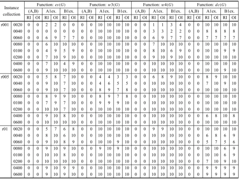
1. We used the first ten graph pairs of the sets r001,r005andr01, with orders 20 ≤ n ≤ 600, indicated as isomorphs in the category randomly connected graphs, from Santoet al. [32] database. We also processed pairs indicated as xxA/xxB1ex and xxA1ex/xxB (where the suffix 1exindicates almost-isomorphic with one 2-exchange), obtained from the corresponding xxA and xxB original graphs.

2. We generated almost-isomorphs with one 2-exchange for two sets of 19 strongly regular graphs [20] of 45 and 64 vertices (numbered 001-019), each graph being tested along with its almost-isomorph. The invariant obtained discrimination in all cases, using the functions w3(G)andw4(G), thedc(G)function was not efficient in these cases.

Table 7.1 indicates the number of pairs (out of 10) from Test 1, for which there was discrimi-nation, both for therelaxed instances(RI)and theoriginal ones(OI). The pairs (A, B) are the original graph pairs, while the suffix “1ex.” indicates one 2-exchange in A or B file. There was no discrimination between the original pairs.

Table 7.1– Results obtained with Santoet al.database.

Instance Function:es(G) Function:w3(G) Function:w4(G) Function:dc(G) collection (A,B) A1ex. B1ex. (A,B) A1ex. B1ex. (A,B) A1ex. B1ex. (A,B) A1ex. B1ex.

RI OI RI OI RI OI RI OI RI OI RI OI RI OI RI OI RI OI RI OI RI OI RI OI

r001 0020 0 0 2 2 0 0 0 0 10 10 10 10 0 0 1 1 3 4 0 0 10 10 10 10

0040 0 0 0 0 0 0 0 0 10 10 10 10 0 0 3 3 2 2 0 0 8 8 8 8

0060 0 0 6 9 7 7 0 0 10 10 10 10 0 0 6 9 7 7 0 0 7 7 7 7

0080 0 0 6 10 10 10 0 0 10 10 10 10 0 0 7 10 10 10 0 0 10 10 10 10

0100 0 0 4 9 5 9 0 0 10 10 10 10 0 0 8 10 6 9 0 0 10 10 9 9

0200 0 0 7 10 9 10 0 0 10 10 10 10 0 0 9 10 9 10 0 0 10 10 10 10

0400 0 0 7 10 4 9 0 0 10 10 10 10 0 0 10 10 10 10 0 0 10 10 10 10 0600 0 0 9 10 10 10 0 0 10 10 10 10 0 0 10 10 10 10 0 0 10 10 9 10

r005 0020 0 0 5 8 7 10 0 0 4 4 3 3 0 0 6 8 9 10 0 0 8 9 10 10

0040 0 0 9 10 7 10 0 0 4 6 5 5 0 0 10 10 10 10 0 0 7 10 9 10

0060 0 0 9 10 7 10 0 0 8 9 7 8 0 0 10 10 10 10 0 0 10 10 10 10

0080 0 0 8 9 9 10 0 0 8 9 7 8 0 0 10 10 10 10 0 0 10 10 10 10

0100 0 0 7 9 7 10 0 0 9 9 9 10 0 0 10 10 10 10 0 0 10 10 10 10

0200 0 0 10 10 7 10 0 0 10 10 10 10 0 0 10 10 10 10 0 0 10 10 10 10

0400 0 0 9 10 8 10 0 0 10 10 10 10 0 0 10 10 10 10 0 0 6 8 10 8

0600 0 0 10 10 10 10 0 0 10 10 10 10 0 0 10 10 10 10 0 0 10 10 10 10

r01 0020 0 0 5 7 6 8 0 0 10 10 10 10 0 0 9 9 10 10 0 0 10 10 10 10

0040 0 0 8 10 6 10 0 0 10 10 10 10 0 0 10 10 10 10 0 0 6 8 6 9

0060 0 0 9 10 8 9 0 0 10 10 9 10 0 0 10 10 10 10 0 0 5 7 5 6

0080 0 0 9 10 9 10 0 0 9 10 9 10 0 0 10 10 10 10 0 0 10 10 6 9

0100 0 0 10 10 8 10 0 0 10 10 10 10 0 0 10 10 10 10 0 0 10 10 6 9 0200 0 0 10 10 10 10 0 0 10 10 10 10 0 0 10 10 10 10 0 0 7 10 9 10

0400 0 0 9 10 9 9 0 0 10 10 10 10 0 0 10 10 10 10 0 0 9 9 9 9

(18)

The results from Test 2, with strongly regular graphs and their almost-isomorphs, are indicated in Table 7.2:

Table 7.2– Results for strongly regular graphs.

Instance w3(G) w4(G) dc(G)

RI OI RI OI RI OI

(45,12,3,3) 19 19 19 19 0 0

(64,18,2,6) 19 19 19 19 0 0

7.1.2 We applied the algorithm VF2 [33] to regular graphs of order 100, 200 and 500 from the database already used in this work. We created isomorphs for these graphs and formed pairs (graph, isomorph). We also used the same one 2-exchange (graph, almost-iso-morph)pairs referred to in Table 4.1 (a).

For the application of VF2 to our instances we used the IGRAPH library [21], version 0.5.4, a free software package for creating and manipulating undirected and directed graphs which contains the VF2 algorithm. All instances were put in Dimacs format and submitted to VF2.

In order to compare the runtime of our algorithm with the library VF2, we needed a maximum time limit for large instances. However, IGRAPH is a closed pack which only stops when it finishes processing. To guarantee a time limit, we created two jobs (shell) using Linux OS. The first shell(JOB1.sh), controls the time limit and the second shell(JOB2.sh)uses the VF2 library in order to check all instances for isomorphism.

IfJOB1.shfinishes first, then JOB2.sh execution time is equal or greater than the time limit and JOB1.sh interrupts both child processes. If, on the contrary, JOB2.shfinishes within the time limit, it interruptsJOB1.shexecution before stopping. See Figure 7.1.

all instances

the existence of the instance in the current directory JOB2 control file

VF2 library

the existence of the control files they exist then

control files child process of JOB1.sh for

for all instances

the maximum processing time the existence of the control files if they exist then

control files both child processes for

all instances

VF2 library

all instances

VF2 library

for all instances

Figure 7.1– Pseudocodes of JOB1 and JOB2 (shells).

Tables 7.3 and 7.4 show the results for each (n,d)ten-graph collection, both for QAPV and VF2, respectively with isomorphic and almost-isomorphic pairs. The maximum processing time allowed for VF2 was 3,600 seconds. All times are expressed in seconds.

(19)

Table 7.3– QAPV-VF2 comparison of processing time with isomorphic pairs.

Instance QAPV VF2

n,d avg, dc avg 6avg max min avg max min

100,3 0.011 0.001 0.012 0.020 0.008 0.158 0.484 0.001 100,10 0.014 0.002 0.016 0.026 0.011 0.075 0.246 0.003 100,25 0.017 0.008 0.025 0.036 0.021 0.123 0.448 0.001 100,50 0.021 0.029 0.050 0.066 0.046 0.303 0.839 0.016 200,3 0.039 0.001 0.040 0.050 0.036 98.903 472.88 0.002 200,10 0.039 0.005 0.044 0.060 0.040 10.017 85,347 0.004 200,25 0.054 0.029 0.083 0.118 0.058 3.086 25.887 0.011 200,50 0.090 0.104 0.194 0.207 0.187 4.734 37.423 0.003 200,100 0.121 0.401 0.522 0.548 0.518 7.636 26.424 0.038 500,3 0.827 0.004 0.831 0.849 0.813 – >3600 548.87 500,10 0.973 0.029 1.002 1.016 0.992 – >3600 41.68 500,25 1.076 0.150 1.226 1.248 1.214 – >3600 61.79 500,50 0.818 0.610 1.428 1.459 1.401 220.83 997.65 3.82 500,100 4.536 2.369 6.905 6.994 6.870 497.49 2294.8 0.165 500,200 17.735 9.440 27.175 27.437 26.719 598.26 2122.8 26.44

Table 7.4– QAPV-VF2 comparison of processing time with almost-isomorphic pairs.

Instance QAPV VF2

n,d avg dc* avg qapv 6avg max min avg max min

100,3 0.010 0.000 0.010 0.021 0.006 0.454 2.372 0.000 100,10 0.013 0.002 0.015 0.026 0.011 0.137 0.485 0.015 100,25 0.016 0.007 0.023 0.032 0.021 0.442 1.596 0.010 100,50 0.021 0.027 0.048 0.063 0.044 1.730 2.916 0.344 200,3 0.038 0.001 0.039 0.049 0.034 68.863 368.28 0.446 200,10 0.039 0.005 0.044 0.061 0.040 6.605 26.078 0.156 200,25 0.053 0.003 0.056 0.084 0.033 4.409 18.404 0.434 200,50 0.091 0.100 0;191 0.204 0.185 3.149 12.725 0.240 200,100 0.120 0.392 0.512 0.530 0.506 18.533 39.091 3.281 500,3 0.819 0.003 0.822 0.848 0.772 – >3,600 45,573 500,10 0.975 0.026 1.001 1.018 0.991 – >3,600 10,617 500,25 1.072 0.153 1.225 1.240 1.218 – >3,600 8,836 500,50 0.822 0.603 1.426 1.453 1.405 – >3,600 20,519 500,100 4.527 2.346 6.873 6.891 6.869 1215,46 1776,56 6,921 500,200 17.787 9.370 27.157 27.215 27.029 – >3,600 117,87

(20)

The last three columns indicate the average, minimum and maximum processing times obtained by the algorithm VF2. Where an instance exceeded the time limit, the average time for its col-lection was not calculated.

8 CONCLUSIONS AND DIRECTIONS FOR FUTURE WORK

Within the orders and degrees studied, the results obtained are in accordance with Conjecture 4.1, the set of functions here proposed allowing us to discriminate between every graph pair used in the tests. We can see thatdc(G)had a complementary performance with respect tow3(G)and w4(G). On the other hand,es(f(G))enhancedw3(G)andw4(G)performances in most cases at a very low additional cost.

We used regular graphs in the majority of the tests because they seem to present a more difficult problem than general graphs, owing to their structure restrictions. Nevertheless, general graphs could also be examined, the technique presenting no restriction concerning degree sequences, as it can be seen with the public instances we tested. For general graphs, es(G)could be applied directly, which would mean much lower computing times.

The study shown here can be extended through the use of new weight function criteria and more efficient programming, especially for the walk-counting techniques. Interesting possibilities are brought by the matrices shown in [6]. It can be applied to other graph families, such as gen-eral planar graphs and trees. We also think that QAPV can be advantageously applied as a first resource to detect non-isomorphic pairs when generating given graph families, VF2 or another exact algorithm taking over the doubtful cases.

The relation between degree and number of centers for regular graphs (indc(G)calculation) is a subject that could lead to interesting theoretical studies. However, they are not within the scope of this paper.

The es(G) function, even when applied twice as in the planar examples, is very quick when compared with the QAP instance processing for the instances examined above 30,000 vertices.

The variance calculation times from Figure 4.2 are those of the original variance, the relaxed one being much less time-consuming. By starting with the relaxed instance, one can then expect to work with bigger graphs much more quickly.

Working with big planar graphs opens possibilities to apply the technique to pattern recognition problems, allowing for quantification of the differences between pairs of images.

It is interesting to observe that, if Conjecture 4.1 could be proven, this would be equivalent to establishing the complexity of the restricted graph isomorphism problem as being polynomial for all graphs.

(21)

REFERENCES

[1] ABREU NMM, BOAVENTURA-NETTO PO, QUERIDO TM & GOUVˆEA EF. 2002. Classes of quadratic assignment problem instances: isomorphism and difficulty measures using a statistical approach.Discrete Applied Mathematics,124: 103–116.

[2] ARVINDV & THORAN´ J. 1985. Isomorphism testing: perspective and open problems. The Compu-tational Complexity Column.Bulletin of the European Association for Theoretical Computer Science,

86: 66–84. In: http://theorie.informatik.uni-ulm.de/Personen/jt.html. Consulted June 2010.

[3] ANGELR & ZISSIMOPOULOSV. 1998. On the quality of the local search for the quadratic assign-ment problem.Discrete Applied Mathematics,82: 15–25.

[4] BOAVENTURA-NETTO PO & ABREU NMM. 1997. Cost solution average and variance for the quadratic assignment problem: a polynomial expression for the variance of solutions. Actas de Resumenes Extendidos, 408–413, I ELIO/Optima 97, Concepci ´on, Chile.

[5] BOAVENTURA-NETTO PO. 2012. Grafos: Teoria, Modelos, Algoritmos (in Portuguese). 5th ed., Edgard Bl¨ucher, S˜ao Paulo. http://www.po.coppe.ufrj.br/docentes/boaventura/home.html.

[6] BESSAAD, ROCHA-NETOIC, PINHOSTR, ANDRADERFS & PETITLOBAO˜ TC. 2012. Graph cospectrality using neighborhood matrices.Electronic Journal of Combinatorics,19(3): 23.

[7] CVETKOVICD, ROWLINSONP & SIMICS. 1997. Eigenspaces of graphs, Cambridge University Press, Cambridge.

[8] CROSSADJ, WILSONRC & HANCOCKER. 1997. Inexact graph matching using genetic search. Pattern Recognition,30(6), 953–970.

[9] CZERWINSKIR. 2010. A polynomial time algorithm for graph isomorphism. http://arxiv.org/pdf/0711.2010v4. Consulted August 2011.

[10] DEPIEROF & KROUTD. 2003. An algorithm using length-r paths to approximate subgraph iso-morphism.Pattern Recognition Letters,24: 33–46.

[11] DINGH & HUANGZ. 2009. Isomorphism identification of graphs: especially for the graphs of kine-matic chains.Mechanism and Machine Theory,44: 122–139.

[12] DOUGLASB. 2011. The Weisfeiler-Lehman method and graph isomorphism testing. http://arxiv.org/pdf/1101.5211v1. Consulted August 2011.

[13] DHARWADKER A & TEVET J. 2009. The graph isomorphism algorithm. In Proceedings of the Structure Semiotics Research Group. Eurouniversity Tallinn. Also in

http://www.dharwadker.org/tevet/isomorphism/. Consulted June 2010.

[14] FOGGIA P, SANSONE C & VENTO M. 2001. A performance comparison of five algorithms for graph isomorphism. Proc. of the 3rd. IAPR-TC-15 International Workshop on Graph-based Repre-sentations, Venice, Italy.

[15] GAREYMR & JOHNSONDS. 1979. Computers and intractability: a guide to NP-completedness. W.H. Freeman.

[16] GORIM, MAGGINIM & SARTI L. 2001. Graph matching using random walks. Proc. of the 3rd. IAPR-TC-15 International Workshop on Graph-based Representations, Venice, Italy.

(22)

[18] GROSSJL & YELLENJ. (eds.) 2005. Handbook of graph theory, CRC Press LLC, Boca Raton.

[19] HARARYF. 1971. Graph theory, Addison-Wesley, Reading, Massachussetts.

[20] HAEMERSWH & SPENCEE. 2001. The pseudo-geometric graphs for generalized quadrangles of order .3.European J. Combin.,22(6): 839–845.

[21] IGRAPHLIBRARY. http://igraph.sourceforge.net/ Consulted June 2012.

[22] JAINBJ & WYSOTSKIF. 2005. Solving inexact graph isomorphism problems using neural networks. Neurocomputing,63: 45–67.

[23] KNUTH D. 1997. The art of computer programming, vol. 2, Seminumerical algorithms. 3rd ed., Addison-Wesley, Reading, Massachussetts.

[24] LOIOLAEM, ABREUNMM, BOAVENTURA-NETTOPO, HAHNP & QUERIDOTM. 2007. A sur-vey for the quadratic assignment problem.European J. of Operational Research,176: 657–690.

[25] LEEL, RANGELMC & BOERESMCS. 2007. Reformulação do problema de isomorfismo de grafos como o problema quadrático de alocação (in Portuguese), Anais do XXXIX SBPO, 1601–1612, Fortaleza.

[26] MELOVA, BOAVENTURA-NETTOPO, HAHNP & BAHIENSEL. 2010. Graph isomorphism and QAP variances.Combinatorial optimization in practice,8(2): 209–234.

[27] MCKAYB. 1981. Practical graph isomorphism.Congressus Numerantium,30(1): 45–87.

[28] MARSAGLIAG. 1984. A current view of random number generators. Keynote address, Proc. 16th Symposium on the Interface, Atlanta. Elsevier.

[29] PORUMBEL DC. 2011. Isomorphism testing via polynomial-time graph extensions. Journal of Mathematical Modelling and Algorithms,10(2): 119–143.

[30] PRESA JLL. 2009. Efficient algorithms for graph isomorphism testing. D.Sc. Thesis, Universidad Rey Juan Carlos, Madrid.

[31] SANTOSPLF. 2010. Teoria espectral de grafos aplicada ao problema de isomorfismo de grafos (in Portuguese). M.Sc. Dissertation, Department of Informatics, Federal University of Esp´ırito Santo, Brazil.

[32] SANTOMDE, FOGGIAP, SANSONEC & VENTOM. 2003. A large database of graphs and its use for benchmarking graph isomorphism algorithms.Pattern Recognition Letters,24: 1067–1079.

[33] http://www.cs.sunysb.edu/∼algorith/implement/vflib/implement.shtml. Consulted May 2012.

[34] VOSS S & SUBHLOK J. 2010. Performance of general graph isomorphism algorithms. Technical Report Number UH-CS-09-07, Department of Computer Science, University of Houston, Houston,