doi: 10.1590/0101-7438.2014.034.03.0647
BUNDLE METHODS IN THE XXIst CENTURY: A BIRD’S-EYE VIEW
Welington de Oliveira
1and Claudia Sagastiz´abal
2*Received September 30, 2013 / Accepted December 12, 2013
ABSTRACT.Bundle methods are often the algorithms of choice for nonsmooth convex optimization, es-pecially if accuracy in the solution and reliability are a concern. We review several algorithms based on the bundle methodology that have been developed recently and that, unlike their forerunner variants, have the ability to provide exact solutions even if most of the time the available information is inaccurate. We adopt an approach that is by no means exhaustive, but covers different proximal and level bundle methods dealing with inexact oracles, for both unconstrained and constrained problems.
Keywords: bundle methods, inexact oracles, nonsmooth convex optimization.
1 INTRODUCTION
Nonsmooth convex optimization (NCO) appears often in connection with real-life problems that are too difficult to solve directly and need to be decomposed. Typically, Lagrangian relaxation or Benders’ decomposition approaches replace the hard problem by a sequence of simpler problems, corresponding, in general, to an iteration of some nonsmooth convex method.
As in Nonlinear Programming, NCO methods define iterates usingoracleinformation, which in the nonsmooth setting comes in the form of a function value and a subgradient. When dealing with the hard problems mentioned above, usually the oracle information cannot be computed exactly (the procedure may be too time consuming, or just impossible, for example, if differential equations or continuous stochastic processes are involved). We refer to this situation as dealing with aninexact oracle; for many examples in the energy sector, see [49].
In 1975 Claude Lemar´echal and Philip Wolfe independently created bundle methods to minimize a convex function for which only one subgradient at a point is computable, [29] and [54]. The short “historical” story [39] discusses the different developments that resulted in theV U-bundle variants [38], that are superlinearly convergent with respect to so-called serious steps. Such a
*Corresponding author.
convergence rate was once deemed unattainable for nonsmooth functions, thus explaining the “science fiction” wording in the title of [39].
Since their introduction, and for practically 25 years, the convergence theory of bundle meth-ods could only handleexactoracles. It was only in 2001 that the work [17] opened the way to inexactness. It was followed by [53] and [27].
For a long time bundle algorithms have been considered as the methods of choice for NCO problems requiring reliable and accurate solutions. The added ability of handling inexact oracles made the new variants even more interesting for real-life applications, especially those involving stochastic programming models. Works such as [43, 44, 2] give a flavor of the many different ways oracle inexactness can be exploited within a bundle method – to eventually solve the hard problem in anexactway. As shown by the numerical experience in [43], for a large battery of two-stage stochastic linear programs it is possible to save up to 75% of the total computational time (while still finding an exact solution) just by letting the bundle method control how accurate the oracle information should be at consecutive iterates. The main idea is that there is no gain in “wasting” time by computing exact oracle information at the so-called null steps; we do not enter into more details here, but refer instead to [43].
In this work we focus on the main ideas behind several variants of bundle methods, rather than on technicalities or fine details. After laying down a minimal background in Section 2, we consider separately unconstrained and constrained methods in Section 3 and 4, respectively. To illustrate the importance of modeling when solving real-life optimization problems, Section 5 contains an example of hydroreservoir management that can be cast into two different formulations, calling for unconstrained or constrained methods. Section 6 concludes with some closing remarks and comments on future research.
2 ORACLE ASSUMPTIONS AND ALGORITHMIC PATTERN
As explained in [48], the versatility of bundle methods dealing with inexact oracles is best ex-ploited when thestructureof the NCO problem is taken into account. For this reason, we con-sider below two structured optimization problems, defined over a polyhedral setX ⊂ ℜn and involving two convex functions, f : ℜn→ ℜandh: ℜn→ ℜ, possibly nonsmooth:
• unconstrained or linearly constrained problem
υopt:=min
x f(x)+h(x) s.t. x∈X. (1a)
• problem with nonlinear convex constraints
υopt :=min
The interest in considering separately the two functions f andhlies in their oracles. More pre-cisely, the function f iseasy: for each givenxk ∈Xthe f-oracle provides
the exact value of the function f(xk) ,
and an exact subgradient gk∈∂f(xk) . (2)
In contrast, the functionhishardto evaluate and, hence, only approximate values are available. Accordingly, at any given pointxk ∈Xtheh-oracle outputs the estimates
hkx =h(xk)−ηhk,
sk ∈ ℜn such that h(·)hkx+
sk,· −xk−η+,
(3)
where the errorsηkhandη+can be unknown. It follows from the oracle definition thath(xk)
hkx+
sk,xk−xk−η+=h(xk)−(ηkh+η+), showing thatηkh+η+≥0. Hence, the approximate subgradient is an(ηhk+η+)-subgradient ofhatxk:
∀x ∈ ℜn h(x)≥h(xk)+sk,x−xk−(ηk
h+η+) with ηhk+η+≥0.
An exact oracle corresponds toηkh =η+ =0. When onlyη+ =0, the oracle is said to be of thelowertype: the linearization generated with the oracle information stays below the function everywhere. In contrast, whenη+>0, the oracle is of the upper type, and the linearizations may cut off portions of the graph ofh. Several examples of such oracles are given in [44]; we just mention here that Lagrangian relaxation is a typical source of oracles of the lower type.
Algorithms in the bundle family use oracles (2) and (3) to define linearizations at iteratesxj, for instance
⎡
⎢ ⎢ ⎣
¯
fj(x) := f(xj)+gj,x−xj ¯
hj(x) := hxj +
sj,x−xj
(f+h)j(x) := f(xj)+hxj +
gj+sj,x−xj.
(4)
At thek-th iteration, the bundle is defined by past oracle information accumulated in some index set Jk ⊂ {1,2, . . . ,k}. Putting together the corresponding linearizations gives cutting-plane models, which can be built individually for each function, or for their sum:
⎡
⎢ ⎢ ⎣
ˇ
fk(x) := maxj∈Jk f¯j(x) (≤ f(x)) ˇ
hk(x) := maxj∈Jk h¯j(x) (≤h(x)+η+)
(f+h)k(x) := maxj∈Jk (f+h)j(x) (≤ f(x)+h(x)+η+) .
(5)
By definition, the models above are piecewise linear convex functions.
minimization of an abstract objective functionOk, depending on a parameter setpars, specific to each considered bundle variant. Accordingly, the next iterate is given by
xk+1∈arg minOk(x;pars) s.t. x∈X. (6)
Typically, the bundle-variant-dependent setparscontains
• the convex model
(f+h)k of f +h(or the sum of models fˇk andhˇkof f andh);
• a stability centerxˆk, usually an element in the sequence{xk}, together with a test to deter-mine when the center can be updated (for example, toxk+1);
• an optimality measure to stop the iterations (such as upper and lower bounds for the opti-mal value of the problem);
• certain algorithmic parameters, to be updated at each iteration.
The main concern when specifying (6) is that the corresponding subproblem is easy, because it needs to be solved at each iteration of the bundle method. A simple illustration, not belonging to the bundle family but still fitting the abstract format above, is the cutting-plane method of [9] and [19], with subproblems fully characterized by
pars:=
(f+h)k and Ok(x;pars):=
(f+h)k(x)
yielding a linear programming problem (LP) in (6):
xk+1∈arg min
(f+h)k(x) s.t. x∈X
(recall the setX is defined by linear equality and inequality constraints.) Bundle methods can be seen as stabilizedforms of the cutting-plane algorithm, well known for its instability and slow convergence. Different stabilization devices result in different bundle algorithms, such as the proximal variant [33] or the level one [30]. For these methods, the respective parameter sets
pars involve more objects than just
(f+h)k and, as shown in Sections 3 and 4 below, give quadratic programming (QP) subproblems (6).
Once the parameter set and the modeling objective function in (6) are specified, the method needs to define updating rules for the elements inpars, including a stopping test. The main steps of all the algorithms are given below.
Algorithmic Pattern 1.Oracles for f and h, a modelOk, and a rule for defining the parameter setparsare given.
STEP0. For an initial iterate x1, call the oracles to obtain the information(f(x1),g1)and
(h1x,s1). Set k=1and initializeJ1= {1},xˆ1=x1.
STEP 2. Perform a stopping test based on the optimality measure inpars.
STEP 3. If xk+1was not considered close enough to optimal, call the oracles at xk+1to obtain the information
(f(xk+1),gk+1) and (hk+1x ,sk+1) .
STEP 4. Depending on a test measuring progress towards the goal of solving(1), specified in
pars, decide whether or not the stability center is to be replaced:
setxˆk+1∈X.
STEP 5. Updateparsby the given rule. Increase k by 1 and loop to Step 1.
The above pattern is merely a sketch of an algorithm. Different models and different updating rules for the stability center define different methods. The stopping test performed in Step 2 depends, naturally, on the bundle method variant. In what follows we will make each Step in the Algorithmic Pattern 1 more precise, for different bundle method variants. In order to ease the presentation, we split our analysis into the two instances considered in (1), starting with the linearly constrained problem (1a).
3 UNCONSTRAINED OR LINEARLY CONSTRAINED SETTING
The algorithms considered in this section are suitable for problems with simple constraints (such as linear) or none at all, as in (1a). We start with the most well known variant, the proximal bundle method, [32, 25, 33, 15]; see also [37, 17, 53, 7, 38, 27, 24, 11, 45, 34, 44, 50].
3.1 Proximal Bundle Methods
This family defines subproblems based on the equivalence between minimizing a convex function and finding a fixed point of the proximal point operator, [40]:
¯
xsolves (1a) ⇐⇒ ¯xsolves min
x∈X f(x)+h(x)+
1 2t|x− ¯x|
2 M,
for some proximal stepsizet >0 and a norm induced by a positive definite matrixM. To make the equivalence above implementable, methods in this variant replacex¯by the current stability center and f +h by some model, which canaggregatethe linearizations and use
(f+h)k, or
disaggregatethe information and use individual cutting-plane models for f andh:
pars=
⎧ ⎪ ⎪ ⎪ ⎪ ⎪ ⎪ ⎪ ⎨
⎪ ⎪ ⎪ ⎪ ⎪ ⎪ ⎪ ⎩
model
(f+h)k if aggregate variant ˇ
fk+ ˇhk if disaggregate variant stability center xˆk ∈ {xk}
Instead of the M-norm, the generalized bundle methods [15] use as stabilizing term a closed convex function satisfying certain properties.
The corresponding QP subproblems (6) are
• Aggregate model:Ok(x;pars)=
(f+h)k(x)+2t1 k|x− ˆx
k|2 M. • Disaggregate model:Ok(x;pars)= ˇfk(x)+ ˇhk(x)+2t1k|x− ˆxk|2M.
Since the objective function in both subproblems is strongly convex, the new iteratexk+1defined by (6) is unique.
Depending on the structure of the problem to be solved, other modeling choices are possible. In [50], for instance, the hard function is the composition of a smooth mapping with a positively homogeneous convex function. The model in pars results from composing a cutting-plane model of the latter with a first Taylor expansion of the former (at the current stability center). Telecommunication networks often exhibit separable structure, that is exploited in [16] via a special Dantzig-Wolfe decomposition approach and in [31] by using a model that sums a cutting-plane model of the hard function and a a second order expansion of the (smooth) easy term. For simplicity in what follows we focus on a proximal bundle variant using the aggregate model (f+h)kand| · |M = | · |, the Euclidean norm.
Subproblem definition
We now provide all the necessary ingredients to make the Algorithmic Pattern 1 an imple-mentable method, when the proximal subproblem uses the aggregate model, so that (6) becomes
xk+1=arg min x∈X
(f+h)k(x)+ 1
2tk
x− ˆx
k
2
, (7)
and the unique solution to (7) is
xk+1= ˆxk−tk(Gk+Nk) with
⎧ ⎪ ⎪ ⎪ ⎨
⎪ ⎪ ⎪ ⎩
Gk := j∈Jk
αkj(gj +sj)∈∂
(f+h)k(xk+1)
Nk := −x
k+1− ˆxk
tk
−Gk ∈∂iX(xk+1),
(8)
whereiX denotes the indicator function of the setX. As for the simplicial multiplierαk in (8),
it satisfies, for all j∈Jk:
j∈Jk
αkj =1, αkj ≥0, αkj[
(f+h)k(xk+1)−(f+h)j(xk+1)] =0.
The resultingselection mechanism takes in Step 5 of the Algorithmic Pattern 1 a bundle set satisfying
Jk+1⊃ {j∈Jk :αkj >0} ∪ {k+1} to define the next model
(f+h)k+1given in (5). An even more economical bundle, called com-pressed, can be built using the aggregate linearization defined in (11) below. As shown in [27] and [44], these strategies save storage without impairing convergence.
Stability Center and Optimality Certificate
The rule to update the stability centerxˆk must assess the quality of the candidatexk+1in terms of the goal of solving (1a). Therefore, if the iteratexk+1provides enough decrease with respect to the “best” available value, f(xˆk)+hkxˆ, the stability center is changed toxk+1. In the bundle jargon settingxˆk+1=xk+1is called making a “serious” step. This occurs when, for an Armijo-like parameterm∈(0,1),
f(xk+1)+hk+1x ≤ f(xˆk)+hkxˆ−mf(xˆk)+hkxˆ−
(f+h)k(xk+1). (9) The rightmost term above is a predicted improvement in the sense that it measures the dis-tance between the best available value f(xˆk)+hkxˆ and the best value predicted by the model, (f+h)k(xk+1).
In this variant, the certificate of optimality depends on two terms, the predicted improvement employed in (9) and the direction, given by the sum of the gradient and the normal element in (8). The following object combines both terms
φk:=(f(xˆk)+hkxˆ)−
(f+h)k(xk+1)+xk+1,Gk+Nk, (10)
and ensures convergence of the method whenever there exists a subsequence{(φk,Gk+Nk)}k∈K that converges to(φ,0), for someφ≤0, [44, Theorem 3.2]. For this reason, an optimality mea-sure for proximal bundle algorithms is to require bothφk ≤0 and
Gk+Nk
to be sufficiently
small. When the serious-step sequence is bounded, this test boils down to the more traditional criterion, that checks if the approximate subgradientGk +Nk ∈∂ǫk
(f+h)+iX
(xˆk)is small enough, whereǫk ≥0, which depends on the errorsηh+η+, must also be sufficiently small.
Impact of inexactness
When the hard functionh is exactly evaluated, or the oracle is of lower type, the definition of
Gk+Nkin (8) implies that theaggregate linearizationstays always below the sum of functions: (f+h)a(x):=
(f+h)k(xk+1)+Gk+Nk,x−xk+1≤ f(x)+h(x) for all x∈X. (11) In particular, the predicted improvement employed in (9) is always nonnegative for exact oracles and so is the difference f(xˆk)+hkxˆ−(f+h)a(xˆk). In contrast, for lower and upper oracles the difference satisfies only the inequality
Such difference can be negative, entailing difficulties in the convergence analysis. In order to overcome this drawback, whenever this difference is too negative the prox-parameter can be increased in Step 2 of the Algorithmic Pattern 1, as in [27]. The following related rule, based on a relative criterion, was considered in [3] and [44]:
whenever (f(xˆ k)+hk
ˆ
x)−(f+h)a(xˆk)
tk
Gk+Nk
2 ≤ −β settk =10tkand loop to Step 1, (12)
for a parameterβ ∈ (0,1)chosen at the initialization step. By making use of the above simple rule, and preventingtk from decreasing before getting a “good candidate”xk+1, the proximal bundle algorithm remains convergent. Clearly, convergence is ensured up to the oracle accuracy: the “optimal” value found by the algorithm has an error not larger than the precisionηh+η+. Thepartly asymptotically exactvariants let the accuracy vary with the iterates in a manner that drivesηkh+ηk+to 0 at serious steps, hence yielding exact solutions in the limit; we refer to [44] for further information.
It is often the case that the QP subproblem solution takes a significant proportion of the total computational time. The aggregate linearization (11) plays an important role for controlling the QP size and making iterations less time consuming. Proximal bundle methods, and some level variants with restricted memory, work with models in (5) whose index setJkcan becompressed in Step 5 of the Algorithm Pattern 1. More precisely, for convergence purposes, it is enough to include in the new bundle setJk+1the linearization of the last iterate and the aggregate lin-earization (11). Nevertheless, the speed of convergence may be impaired if the bundle is too economical; in this case, the selection mechanism may offer a better trade-off between number of iterations to reach convergence and the time spent in each individual iteration.
3.2 Level Bundle Methods
The level bundle method was proposed in [30] for convex unconstrained and constrained opti-mization problems, saddle-point problems, and variational inequalities. When compared to the proximal family, the level class can be considered as making primal-dualapproximations, in the following sense. Start by rewriting the proximal point operator equivalence, multiplying the minimand therein by the positive factort:
¯
xsolves (1a) ⇐⇒ ¯xsolves min
x∈Xt(f(x)+h(x))+
1 2|x− ¯x|
2 M.
Then, interpreting this factor as amultipliergives the relation
¯
xsolves (1a) ⇐⇒ ¯xsolves
⎧ ⎨
⎩
min x∈X
1 2|x− ¯x|
2 M
s.t. f(x)+h(x)≤ f(x¯)+h(x¯) .
Once again, to make the equivalence above implementable, methods in the level variant replace
¯
hand side term in the constraint by alevelparameter. Also, theM-norm is extended to general stability functions derived from a smooth strongly convex functionω: ℜn→ ℜ
+that can yield a subproblem that is conic and no longer quadratic. Typically, the parameter set in the level variant is pars= ⎧ ⎪ ⎪ ⎪ ⎪ ⎪ ⎪ ⎪ ⎪ ⎪ ⎪ ⎪ ⎨ ⎪ ⎪ ⎪ ⎪ ⎪ ⎪ ⎪ ⎪ ⎪ ⎪ ⎪ ⎩ model
(f+h)k if aggregate variant
ˇ
fk + ˇhk if disaggregate variant stability center xˆk∈X,
stability function ω(x)−
∇ω(xˆk),x− ˆxk
, level parameter flevk ∈(flowk , fupk), for lower and upper bounds flowk ≤υoptand fupk ≥υopt.
As mentioned in [6], the functionωcan be chosen to exploit the geometry of the feasible setX (that may be non-polyhedral), to get nearly dimension-independent complexity estimates of the maximum number of iterations necessary to reach an optimality gap fupk −flowk inferior to a given tolerance.
Complexity estimates are obtained if the feasible setXis compact, an assumption present in most level bundle methods, [30, 26, 12, 6, 28, 47]. Level bundle methods able to deal with unbounded feasible sets have an asymptotic analysis instead; we refer to [8, 43, 5, 35] and [12, 43, 35] for variants handling exact and inexact oracles, respectively.
Subproblem Definition
In this case, subproblem (6) has the form
xk+1=arg min x∈X ω(x)−
∇ω(xˆk),x− ˆxk s.t.
(f+h)k(x)≤ flevk . (13)
For the (canonical) stability function ω(x) = 12x,x in particular, subproblem (13) is the quadratic program
xk+1=
⎧ ⎪ ⎪ ⎪ ⎨ ⎪ ⎪ ⎪ ⎩
arg min 12x− ˆxk
2
s.t.
(f+h)k(x)≤ flevk x∈X,
corresponding to the orthogonal projection of the stability centerxˆkonto the polyhedronX∩Xk lev, for
Xlevk :=
x∈ ℜn:
(f+h)k(x)≤ flevk , (14) a nonempty set, since the level parameter flevk ≥minx∈X
(f+h)k(x).
Similarly to the proximal variant, the optimality conditions for the QP subproblem above give an iteratexk+1as in (8), only that nowtkis replaced byµk =j∈Jkαkj and
Gk = 1
µk
j∈Jk
αkj(gj+sj)∈∂
for a Lagrange multiplierαk that is no longer simplicial but conical and satisfies the following relations for all j ∈Jk
j∈Jk
αkj ≥1, αkj ≥0, αkj
(f+h)j(xk+1)− flevk
=0,
Unlike the proximal bundle variant, in the level family the dual variables of problem (13) can be unbounded.
Stability Center and Optimality Certificate
The rule to update the stability centerxˆkis more flexible than in the proximal family. For exact oracles, the initial article [30] sets xˆk = xk for allk and, hence, does not have therestricted memoryfeature: with this approach compression is not possible. The proximal level variant [26] updates the center using the proximal bundle method rule (9) and, as such, works with restricted memory; similarly for [8] and [35]. Finally, [5] keeps the stability center fixed along the whole iterative process by settingxˆk= ˆx1for allk.
The optimality certificate checks the gap between the upper and lower bounds that also define the level parameter
flowk := minx∈X
(f+h)k(x).
fupk := minj≤k{f(xj)+hxj}
⇒ flevk :=γflowk +(1−γ )fupk ,
for some coefficient γ ∈ (0,1). For polyhedral feasible setsX, the computation of the lower bound amounts to solving an LP; for more economical alternative definitions of the lower bound, we refer to [43].
When the feasible setXis compact, the stopping test in Step 2 of Algorithmic Pattern 1 checks if the optimality gap fupk − flowk is below some tolerance. For the unbounded setting the stopping test of the proximal bundle method must be considered as well: stop either when the optimality gap is sufficiently small, or when bothGk+Nk
andφkare small.
Impact of Inexactness
It was shown in [41] that if the feasible set is compact, no additional procedure needs to be done to cope with inexactness from the oracle. The non-compact setting is more intricate. Basically, the level parameter remains fixed when the oracle error is deemed too large, using the test (12) to detect large “noise”. For more information on how to deal with oracle errors in level bundle methods when in (1a) the feasible set is unbounded see [35].
3.3 Doubly Stabilized Bundle Methods
the feasible set is a compact polyhedron. Thedoubly stabilizedbundle method [46] combines in a single algorithm the main features of the proximal and level methods, in an effort to exploit the best features of both variants.
A possible parameter set in this variant is
pars= ⎧ ⎪ ⎪ ⎪ ⎪ ⎪ ⎪ ⎪ ⎪ ⎪ ⎪ ⎪ ⎪ ⎪ ⎪ ⎨ ⎪ ⎪ ⎪ ⎪ ⎪ ⎪ ⎪ ⎪ ⎪ ⎪ ⎪ ⎪ ⎪ ⎪ ⎩ model
(f+h)k if aggregate variant
ˇ
fk + ˇhk if disaggregate variant stability center xˆk∈ {xk},
stability function | · |, prox-stepsize tk>0,
level parameter flevk ∈(flowk , fupk), for lower and upper bounds flowk ≤υoptand fupk ≥υopt.
Subproblem Definition
LettingiXk
lev(·)denote the indicator function of the level set (14), the objective function of
sub-problem (6) is given by
Ok(x;pars)=
(f+h)k(x)+ 1
2tk
x− ˆx
k
2 +iXk
lev(x) .
As long as the level setXk
levis nonempty, the new iterate is given by the following particulariza-tion of subproblem (6):
xk+1=arg min x∈X
(f+h)k(x)+ 1
2tk
x− ˆx
k
2 +iXk
lev(x) , (15)
which can be rewritten as
xk+1 =
⎧ ⎪ ⎪ ⎪ ⎨ ⎪ ⎪ ⎪ ⎩ arg min
(f+h)k(x)+2t1 k
x− ˆxk
2
s.t.
(f+h)k(x)≤ flevk x∈X.
Lemma 2 in [46] shows that the solutionxk+1 of the QP (15) solves either (7) or (13) (when ω(x) = 12x,x in the latter problem), so the doubly stabilized variant indeed combines the proximal and level methods. The numerical experiments reported in [46] show a gain in perfor-mance, likely due to the increased versatility of this variant.
The unique QP solution is characterized as follows; see [46, Prop. 2.1]:
xk+1= ˆxk−tkµk(Gk+Nk) with
⎧ ⎪ ⎪ ⎪ ⎨ ⎪ ⎪ ⎪ ⎩
Gk := 1
µk
j∈Jk
αkj(gj +sj)∈∂
(f+h)k(xk+1)
Nk := −x
k+1− ˆxk
tkµk
The multipliersαk≥0 andµk ≥1 satisfy the following relations for all j ∈Jk
µk =
j∈Jk
αkj, λk=µk−1
αkj
(f+h)k(xk+1)−(f+h)j(xk+1)=0, λk
(f+h)k(xk+1)− flevk =0.
As in the previous methods, theαkj-multipliers can be employed to select active linearizations. With this variant, the compression mechanism is also applicable.
Stability Center and Optimality Certificate
The rule to update the stability centerxˆkis (9), as in the proximal bundle method. The stopping test combines the proximal and level criteria: the algorithm stops when eitherGk+Nk
andφk are small, or when the optimality gap is close to zero.
An additional bonus is that theµk-multipliers can be used to update the prox-stepsize. Specifi-cally, in view of the optimality conditions above, given someγ ∈(0,1), the rule
setstk+1=γtkin case of null step andtk+1=µktkifxk+1is a serious iterate.
Impact of Inexactness
As shown in [46], a distinctive feature of this variant is that it can be employed with both exact or inexact oracles without any changes, as long as the last “proximal step” linearization is kept in the information bundle.
Having laid down the background for problems with simple constraints, we now turn our atten-tion to the constrained problem (1b).
4 CONSTRAINED SETTING
In spite of having only one scalar constraint, formulation (1b) is general and covers problems withmscalar convex constraintshj(x)≤0,j =1, . . .m, just by taking
h(x):= max j=1,...,m
hj(x) .
penalty parameter is sometimes a delicate task. In what follows we focus on methods developed under a different paradigm, making use of improvement functions. For another alternative, we refer to the filter method in [18].
4.1 Improvement Function
When the optimal valueυoptof problem (1b) is known, a direct reformulation of (1b) consists in
minimizing the function max{f(x)−υopt,h(x)}over the setX. Since often the optimal value
is not available, instead one considers approximations of the form
F(x;τ1k, τ2k):=max{f(x)−τ1k, h(x)−τ2k} for targets
τ1k ≈ υopt
τ2k ≈ 0, (16) which will be in turn modeled by cutting-plane functions.
The improvementfunction (16) finds a compromise between optimality and feasibility, repre-sented by the first and second terms in the max-operation, respectively. The target choice depends on the method; [30] takesτ1k := flowk , a lower bound forυopt, and setsτ2k := 0; in [23], the
first target is the sum of the objective function value at the current stability center and a weighted measure of its feasibility; and other rules are considered in [23, 51, 3].
As for the unconstrained case, we revise different bundle variants suited to (1b), starting with the proximal family.
4.2 Constrained Proximal Bundle Methods
The method introduced in [51] takes the current serious step function value for the first target andτ2k=0 and applies an unconstrained proximal bundle method to the function
Fk(x):=maxf(x)− f(xˆk),h(x).
When the next serious iterate is generated, the first target is replaced accordingly, making the necessary changes to the bundle. These changes are not straightforward because, as explained in [51], ensuring descent for the improvement function above does not necessary entail descent for the objective in (1b).
The parameters characterizing this family of methods is
pars=
⎧ ⎪ ⎪ ⎪ ⎪ ⎪ ⎨
⎪ ⎪ ⎪ ⎪ ⎪ ⎩
model k(x):=max{ ˇf(x)− f(xˆk), hˇ(x)}, stability center xˆk ∈ {xk},
stability function | · |the Euclidean norm, prox-stepsize tk >0.
Subproblem Definition
In this variant, the objective function in (6) is
Ok(x;pars)=k(x)+ 1 2tk
x− ˆx
k
yielding a QP problem, with unique solution as in (8) written with∂
(f+h)k(xk+1)therein re-placed by
∂k(xk+1)=
⎧ ⎪ ⎪ ⎪ ⎨
⎪ ⎪ ⎪ ⎩
∂fˇ(xk+1) if fˇ(xk+1)− f(xˆk) >hˇ(xk+1),
conv{∂fˇ(xk+1)
∂hˇ(xk+1)} if fˇ(xk+1)− f(xˆk)= ˇh(xk+1), ∂hˇ(xk+1) if fˇ(xk+1)− f(xˆk) <hˇ(xk+1).
Stability Center and Optimality Certificate
The stability center, which also defines the first target, is changed when the current improvement function is sufficiently reduced using a test akin to (9), i.e.,
Fk(xk+1)≤Fk(xˆk)−m
Fk(xˆk)−k(xk+1)
.
Because the improvement function is a max-function, the test requires progress on both opti-mality and feasibility criteria. Note also that, as Fk(xˆk) = max{0, h(xˆk)}, when the center is infeasible it is possible that f(xˆk+1) > f(xˆk). So, outside the feasible region, the method is not monotone with respect to f but it is monotone with respect toh, thus decreasing infeasibility. The situation is reversed once a feasible stability center is found.
The non-straightforward changes in the bundle alluded above refer to the fact that whenxˆk+1= xk+1, the bundle that was used to model the functionFk must now be adapted to model the new improvement functionFk+1(x) = max{f(x)− f(xk+1), h(x)}. We refer to Section 3 in [51] for details.
Approximate optimality is declared when the center satisfies the inclusionGk+Nk ∈∂ǫkFk(xˆ k) with bothGk+Nk
andǫksufficiently small. When calculations are exact or for inexact oracles with boundedX, this test boils to the one usingφkfrom (10).
Impact of Inexactness
Suppose now the constrainth in (1b) is hard to compute. The ideas above were generalized to handle inexact oracles in [3], using a test similar to (12) mutatis mutandis. The extension addresses two important issues, described below.
• The targets in the improvement function are more general:
τ1k = f(xˆk)+ρkmax{hkxˆ,0} and τ2k=σkmax{hkxˆ,0}
• Rather than requiring descent for the improvement function, the stability center is updated wheneitherthe center is feasible and the new point is feasible and gives descent for the objective function,orthe center is infeasible and the new point reduces infeasibility. This weaker condition is likely to update serious steps more often.
4.3 Constrained Bundle Methods in the Level Family
The first constrained level method able to deal with inexactness was proposed by [12], assuming the oracle is of the lower type with vanishing errors, that isηkh → 0. Further improvements, incorporating the on-demand accuracy setting from [43], were considered in [13]. The basic idea in these articles is to apply some unconstrained level bundle method to solve the linearly constrained problem minx∈XFk(x)where
Fk(x):=F(x; flowk ,0)from (16) and with f k
low↑υopt.
Since the algorithms in [30, 26, 12, 13] make use of certain dual variables to update the level parameter for the cutting-plane model of Fk, below we grouped them in the family of
primal-duallevel bundle methods. In contrast, the methods proposed in [2] do not set the objective function in the subproblems to be Fk but rather use the improvement function as a measure to certify optimality. The authors justify this choice as being more natural when dealing with inexactness from the oracle. The method was extended in [42] to solve convex mixed-integer non-linear programming problems.
For both types of methods, the parameter set is
pars=
⎧ ⎪ ⎪ ⎪ ⎪ ⎪ ⎪ ⎪ ⎪ ⎪ ⎪ ⎪ ⎪ ⎪ ⎪ ⎨
⎪ ⎪ ⎪ ⎪ ⎪ ⎪ ⎪ ⎪ ⎪ ⎪ ⎪ ⎪ ⎪ ⎪ ⎩
models
ˇ
fk for f ˇ
hk forh stability center xˆk ∈X, stability function | · |,
lower bound flowk ≤υopt,
level-parameter flevk ≥ flowk , improvement function Fk.
4.3.1 Primal-Dual Constrained Level Bundle Methods
The algorithms in [30, 12] define the objective function in (6) as
Ok(x;pars)= 1
2
x− ˆx
k
2 +iXk
lev(x) .
In these primal-dual variants, the level setXk
so thatαkfˇk(x)+(1−αk)hˇk(x)is a cutting-plane approximation of the improvement function. Accordingly, the iteratexk+1solves the QP subproblem:
xk+1=
⎧ ⎪ ⎪ ⎨
⎪ ⎪ ⎩
arg min 12x− ˆxk
2
s.t. αkfˇk(x)+(1−αk)hˇk(x)≤ flevk
x ∈X.
The level parameter flevk is updated by solving an LP, as in the unconstrained variant.
Stability Center and Optimality Certificate
The rule proposed in [30] to update the stability center is simple: just take xˆk as the current iteratexk. Differently, [26] updatesxˆkonly after observing enough progress in the improvement functionFk(as for the proximal variants). The new stability center can be any point in the infor-mation bundle (for example, a feasible iterate with lowest objective function value). The choice
ˆ
xk=x1for allkis also possible for the method proposed in [26].
The optimality certificate is given by the improvement function: the algorithm stops with a δTol-solution when minj≤kFk(xj)≤δTol.
Impact of Inexactness
Publication [12] works with lower oracles, soη+≡0, and the algorithm assumes the oracle error ηhkis driven to zero along the iterative process: eventually the method coincides with the variant for exact oracles.
4.3.2 Constrained Level Bundle Methods
The method proposed in [2] defines the objective function in (6) as
Ok(x;pars)= 1 2
x− ˆx
k
2 +iXk
lev(x) ,
where the level setXk
levis the intersection of the level set for the objective model fˇkwith an outer approximation of the constraint set. Accordingly, the next iterate solves the QP subproblem:
xk+1=
⎧ ⎪ ⎪ ⎪ ⎪ ⎪ ⎨
⎪ ⎪ ⎪ ⎪ ⎪ ⎩
arg min 12x− ˆxk
2
s.t. fˇk(x)≤ flevk ˇ
hk(x)≤0
x∈X.
(17)
Lemma 2 in [2] assures that flevk is a lower bound for the optimal valueυoptof (1b) whenever
The rule given in [2] to update the lower bound and the level parameter does not rely on dual variables, and is much simpler:
flevk = flowk +γmin j≤k Fk(x
j )
flowk =
flevk if Xk
levis empty
flowk−1 otherwise.
Different from the primal-dual family, no additional optimization subproblem needs to be solved at each iteration (neither to define the dual variableαknor to obtain flowk ). In this method, both selection and compression of the bundle is possible.
Stability Center and Optimality Certificate
Similar to the unconstrained level bundle method given in [43], a new stability center xˆk is chosen in the information bundle wheneverXk
levis empty. The stopping test is identical to the one in [30, 26, 12], checking that minj≤kFk(xj)is sufficiently small.
Impact of Inexactness
The algorithm is robust to noise, in the sense that no additional test is required to cope with inexactness. With an exact oracle, the improvement function is always nonnegative. Negative values forFk(·)may arise when the oracle is inexact, in which case the method terminates with an(ηh+η++δTol)-solution to problem (1b). For lower oracles, driving to zero the errorηkhfor certain iterates namedsubstantialensures that asymptotically an exact solution is found; [2].
5 ONE PROBLEM, TWO FORMULATIONS
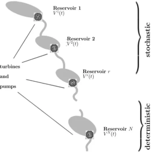
When dealing with real-life problems,modelingis an issue as important as solvingthe result-ing optimization problem. As an illustration, we now consider an example from hydroreservoir management and represent the same physical problem in two different manners, yielding either a problem of the form (1a) or of the form (1b).
Figure 1 represents a set of power plants along a hydrological basin in which the reservoirs uphill have a volume subject to random streamflows due to melted snow. In the figure, there are
Figure 1–Schematic Representation of a Hydrovalley.
In particular, an important concern is to keep the reservoirs above somemin-zoneconstraints, i.e., lower bounds set by the system operator for navigation or irrigation purposes. Since the reservoir volumes are uncertain, so are the min-zones values, and the optimization problem that defines the remuneration for each power plant has a stochastic nature. A possibility to define a turbine throughput and pumping strategy that is suitable for the whole hydrovalley is to endow the optimization problem withprobabilistic constraints.
Suppose a (random) unit priceπ, a (random) lower boundℓ, and a probability level p ∈(0,1) are given. Letting x ∈ Rn denote the abstract vector gathering the decision variables (release water through the turbines, pumping, etc), the hydroreservoir management problem has the form
⎧ ⎪ ⎪ ⎨
⎪ ⎪ ⎩
max π,x
s.t. x∈Xa bounded convex polyhedron, P(ℓ≤x)≥ p.
When streamflows are represented by some autoregressive model with Gaussian innovations, the joint chance constraints above define a convex feasible set and
h(x):=log(p)−logP(ℓ≤x) (18)
96 time steps, the vectorx, formed by subvectors for each plant, each one of lengthT, has a dimension of several hundreds.
We are therefore in our initial setting: the hydroreservoir management problem fits structure (1b) with a linear f(·):= π,·, easy to evaluate, and a difficult constraint of the form (18).
To see how to cast the hydroreservoir problem in the format (1a), we follow [52, Chapter 4.3.2] and consider the set ofp-efficient points, a generalization of thep-quantile:
Zp:=z∈Rn :Fℓ(z)≥ p
whereFℓ(z)=P(x ≥z)is the distribution function of the min-zone boundℓ.
As explained in [52, Chapter 4.3.3], the equivalent reformulation of the hydroreservoir problem
⎧ ⎪ ⎪ ⎪ ⎨
⎪ ⎪ ⎪ ⎩
max π,x
s.t. x∈X
x≥z z∈Zp
can be dualized by introducing Lagrange multipliers 0≤u ∈Rnfor the constraintx ≥ z. The resulting dual problem
min f(u)+h(u)
s.t. u ≥0 with
f(u) := maxx∈Xπ−u,x
h(u) := maxz∈Zpu,z
fits setting (1a). Oracles for estimating the value and gradient of the hard functionh, involving integer programming, are considered in [10].
The loop is looped: starting with a problem as in (1b) we found an equivalent problem in the form (1a). The decision of which formulation to choose to eventually solve the hydroreservoir management problem will depend on the availability of the oracle and NCO solvers. For instance, designing an oracle for (18) requires having a good code for numerical integration while the hard function depending on p-efficient points calls for combinatorial optimization techniques. A final, not less important, consideration is to analyze what is the desiredoutputof the problem (only the optimal value, or a solution, or a feasible point, etc).
6 FINAL COMMENTS
We gave a panorama of state-of-the-art bundle algorithms that were developed in the last 10-15 years to deal with inaccurate oracle information. Applications in energy, finance, transportation or planning often require solving with high precision and in a reliable manner large-scale prob-lems for which the oracle information is hard, if not impossible, to obtain. The new generation of bundle methods reviewed in this work constitutes an important set of optimization tools for such real-life problems.
largely on thestructureof the problem to be solved. For instance, for large-scale unconstrained optimization problems the proximal bundle method seems to be more suitable than the level one, since each iterate can be determined by maximizing a quadratic function over a simplex (this is a QP subproblem, dual to (7)). On the other hand, if the feasible set is bounded, the level bun-dle variant might be preferable because the fact of having a lower bound allows the method to build an optimality gap, a stopping criterion that is easier to satisfy in general. Similarly if the optimal value of the problem is known in advance. The doubly stabilized variant can be a good solver for repeated solution of different types of problems, since it gives an automatic mechanism to combine the advantages of the proximal and level methods for the unconstrained or linearly constrained setting.
Notwithstanding, each bundle variant has parameters to be dealt with, such as the prox-stepsize or the level parameter. The convergence theory for each method relies on the proper updating of such parameters. For the proximal family, for instance, the stepsize cannot increase at null steps and (as for subgradient methods) must form a divergent series. For the level family, flevk is often a convex combination of the current upper and lower bounds. Depending on the updating rule for the lower bound, the level parameter can make the subproblem infeasible. As long as the subproblem is a QP, this is not a major concern: most of modern QP solvers return with an exit flag informing infeasibility. In this case, the lower bound and level parameter are easily updated, see Subsection 4.3.2. Furthermore, to prevent the level set from being empty, the lower bound can be computed by solving an LP at each iteration, as discussed in Subsection 3.2.
An important point to note is that for lower and on-demand accuracy oracles (not for upper oracles), inexact bundle methods can eventually find an exact solution even if the oracle infor-mation is inexact most of time: the solution quality depends only on how accurate the oracle is at serious steps.
Regarding computational packages, several of the variants described above are freely available for academic use upon request to the authors, including [15] and [44].
We finish by commenting on several future directions of research.
For the proximal family, [4] makes a first incursion into new criteria to define stability centers. Differently from (9), the serious sequence may have non-monotone function values. The idea is to have more serious steps and to avoid the algorithm stalling at null steps. It would be interesting to see if it is possible to relate these new criteria to crucial objects in the level family, such as the optimality gap.
by, for instance, looking for the solution that is closest to some reference point. Exploiting the structure in such nonsmooth minimal norm solution problems could lead to the design of new specialized solution algorithms, based on the bundle methodology.
Finally, along the lines of the work [38] for proximal bundle methods, it would be interesting to incorporateV U-decomposition into the level family to device superlinearly convergent level bundle methods.
ACKNOWLEDGMENTS
We are grateful to Robert Mifflin for his careful reading and useful remarks. The second author is partially supported by Grants CNPq 303840/2011-0, AFOSR FA9950-11-1-0139, as well as by PRONEX-Optimization and FAPERJ.
REFERENCES
[1] VANACKOOIJW, HENRIONR, M ¨OLLER A & ZORGATIR. 2013. Joint chance constrained pro-gramming for hydro reservoir management.Optimization and Engineering, accepted for publication.
[2] VANACKOOIJW &DEOLIVEIRAW. 2014. Level bundle methods for constrained convex optimiza-tion with various oracles.Computational Optimization and Applications,57: 555–597.
[3] VANACKOOIJW & SAGASTIZABAL´ C. 2014. Constrained bundle methods for upper inexact oracles with application to joint chance constrained energy problems.SIAM Journal on Optimization,24(2): 733–765. Doi=10.1137/120903099.
[4] ASTORINOA, FRANGIONIA, FUDULIA & GORGONEE. 2013. A nonmonotone proximal bundle method with (potentially) continuous step decisions.SIAM Journal on Optimization,23: 1784–1809.
[5] BELLOCRUZJY &DEOLIVEIRAW. 2014. Level bundle-like algorithms for convex optimization. Journal of Global Optimization,59(4): 787–809.Doi=10.1007/s10898-013-0096-4.
[6] BEN-TALA & NEMIROVSKIA. 2005. Non-euclidean restricted memory level method for large-scale convex optimization.Math. Program.,102: 407–456.
[7] BORGHETTIA, FRANGIONIA, LACALANDRAF & NUCCIC. 2003. Lagrangian heuristics based on disaggregated bundle methods for hydrothermal unit commitment.IEEE Transactions on Power Systems,18: 313–323.
[8] BRANNLUNDU, KIWIELKC & LINDBERGPO. 1995. A descent proximal level bundle method for convex nondifferentiable optimization.Operations Research Letters,17: 121–126.
[9] CHENEY E & GOLDSTEINA. 1959.Newton’s method for convex programming and Tchebycheff approximations,1: 253–268.
[10] DENTCHEVAD & MARTINEZ G. 2003. Regularization methods for optimization problems with probabilistic constraints.Math. Program.,138: 223–251.
[11] EMIELG & SAGASTIZABAL´ C. 2010. Incremental-like bundle methods with application to energy planning.Computational Optimization and Applications,46: 305–332.
[13] F ´ABIAN´ C. 2013.Computational aspects of risk-averse optimisation in two-stage stochastic models, tech. rep., Institute of Informatics, Kecskem´et College, Hungary. Available at:
http://www.optimization-online.org/DB_HTML/2012/08/3574.html.
[14] FISCHER F & HELMBERG C. 2014. A parallel bundle framework for asynchronous subspace optimization of nonsmooth convex functions. SIAM Journal on Optimization, 24(2): 795–822.
Doi=10.1137/120865987.
[15] FRANGIONIA. 2002. Generalized bundle methods.SIAM Journal on Optimization,13: 117–156.
[16] FRANGIONIA & GENDRONB. 2013. A stabilized structured Dantzig Wolfe decomposition method. Math. Program.,140: 45–76.
[17] HINTERMULLER¨ M. 2001. A proximal bundle method based on approximate subgradients. Compu-tational Optimization and Applications,20: 245–266.
[18] KARASE, RIBEIROA, SAGASTIZABAL´ C & SOLODOVM. 2009. A bundle-filter method for nons-mooth convex constrained optimization.Math. Program.,116: 297–320.
[19] KELLEYJ. 1960. The cutting-plane method for solving convex programs.Journal of the Society for Industrial and Applied Mathematics,8: 703–712.
[20] KIWIELK. 1985. An exact penalty function algorithm for nonsmooth convex constrained minimiza-tion problems.IMA J. Numer. Anal.,5: 111–119.
[21] KIWIELK. 1985. Methods of descent for nondifferentiable optimization. Springer-Verlag, Berlin.
[22] KIWIELK. 1991. Exact penalty functions in proximal bundle methods for constrained convex non-differentiable minimization.Math. Programming,52: 285–302.
[23] KIWIEL K. 2008. A method of centers with approximate subgradient linearizations for nonsmooth convex optimization.SIAM Journal on Optimization,18: 1467–1489.
[24] KIWIEL K & LEMARECHAL´ C. 2009. An inexact bundle variant suited to column generation. Math. Program.,118: 177–206.
[25] KIWIELKC. 1995. Approximations in proximal bundle methods and decomposition of convex pro-grams.Journal of Optimization Theory and Applications,84: 529–548. 10.1007/BF02191984.
[26] KIWIELKC. 1995. Proximal level bubdle methods for convex nondiferentiable optimization, saddle-point problems and variational inequalities.Math. Program.,69: 89–109.
[27] KIWIEL KC. 2006. A proximal bundle method with approximate subgradient linearizations.SIAM Journal on Optimization,16: 1007–1023.
[28] LANG. 2013. Bundle-level type methods uniformly optimal for smooth and nonsmooth convex opti-mization.Math. Program., pp. 1–45.
[29] LEMARECHAL´ C. 1975. An extension of Davidon methods to nondifferentiable problems.Math. Programming Stud.,3: 95–109.
[30] LEMARECHAL´ C, NEMIROVSKII A & NESTEROV Y. 1995. New variants of bundle methods. Math. Program.,69: 111–147.
[32] LEMARECHAL´ CANDSAGASTIZABAL´ C. 1994. An approach to variable metric bundle methods. Lecture Notes in Control and Information Science,197: 144–162.
[33] LEMARECHAL´ C & SAGASTIZABAL´ C. 1997. Variable metric bundle methods: From conceptual to implementable forms.Math. Program.,76: 393–410. 10.1007/BF02614390.
[34] LIN H. 2012. An inexact spectral bundle method for convex quadratic semidefinite programming. Computational Optimization and Applications,53: 45–89.
[35] MALICKJ, DE OLIVEIRA W & ZAOURARS. 2013.Nonsmooth optimization using uncontrolled inexact information, tech. rep. Available at:
http://www.optimization-online.org/DB_HTML/2013/05/3892.html.
[36] MIFFLINR. 1977.An algorithm for constrained optimization with semismooth functions,2: 191–207.
[37] MIFFLIN R & SAGASTIZABAL´ C. 2000. OnVU-theory for functions with primal-dual gradient structure.Siam Journal on Optimization,11: 547–571.
[38] MIFFLINR & SAGASTIZABAL´ C. 2005. AVU-algorithm for convex minimization.Math. Program.,
104: 583–608.
[39] MIFFLINR & SAGASTIZABAL´ C. 2012. Optimization Stories, vol. Extra Volume ISMP 2012, ed. by M. Gr¨otschel, DOCUMENTA MATHEMATICA, ch. A Science Fiction Story in Nonsmooth Opti-mization Originating at IIASA, p. 460.
[40] MOREAU J. 1965. Proximit´e et dualit´e dans un espace Hilbertien. Bull. Soc. Math. France, 93: 273–299.
[41] DE OLIVEIRA W. 2011. Inexact bundle methods for stochastic optimization. PhD thesis, Federal University of Rio de Janeiro, COPPE/UFRJ, January 2011. (In Portuguese) Avail-able at: http://www.cos.ufrj.br/index.php?option=com_publicacao&task= visualizar&cid%5B0%5D=2192.
[42] DEOLIVEIRAW. 2014.Regularized nonsmooth methods for solving convexMINLPproblems, tech. rep. Available at:www.oliveira.mat.br.
[43] DE OLIVEIRA W & SAGASTIZABAL´ C. 2014. Level bundle methods for oracles with on-demand accuracy.Optimization Methods and Software,29(6): 1180–1209. Doi=10.1080/10556788. 2013.871282.
[44] DEOLIVEIRAW, SAGASTIZABAL´ C & LEMARECHAL´ C. 2014. Convex proximal bundle methods in depth: a unified analysis for inexact oracles.Mathematical Programming, pp. 1–37. Springer Berlin Heidelberg.Doi=10.1007/s10107-014-0809-6.
[45] DE OLIVEIRA W, SAGASTIZABAL´ C & SCHEIMBERGS. 2011. Inexact bundle methods for two-stage stochastic programming.SIAM Journal on Optimization,21: 517–544.
[46] DEOLIVEIRAW & SOLODOVM. 2013.A doubly stabilized bundle method for nonsmooth convex optimization, tech. rep. Available at:
http://www.optimization-online.org/DB_HTML/2013/04/3828.html.
[47] RICHTARIK´ P. 2012. Approximate level method for nonsmooth convex minimization.Journal of Optimization Theory and Applications,152: 334–350.
[49] SAGASTIZABAL´ C. 2012. Divide to conquer: decomposition methods for energy optimization. Math. Program.,134: 187–222.
[50] SAGASTIZABAL´ C. 2013. Composite proximal bundle method.Mathematical Programming,140: 189–233.
[51] SAGASTIZABAL´ C & SOLODOV M. 2005. An infeasible bundle method for nonsmooth convex constrained optimization without a penalty function or a filter.SIAM Journal on Optimization,16: 146–169.
[52] SHAPIROA, DENTCHEVAD & RUSZCZYNSKI´ A. 2009. Lectures on Stochastic Programming: Mod-eling and Theory. MPS-SIAM Series on Optimization, SIAM – Society for Industrial and Applied Mathematics and Math. Program. Society, Philadelphia.
[53] SOLODOVMV. 2003. On approximations with finite precision in bundle methods for nonsmooth optimization.Journal of Optimization Theory and Applications,119: 151–165.