doi: 10.1590/0101-7438.2014.034.03.0481
CONSTANT RANK CONSTRAINT QUALIFICATIONS: A GEOMETRIC INTRODUCTION
Roberto Andreani and Paulo J.S. Silva*
Received October 19, 2013 / Accepted December 28, 2013
ABSTRACT.Constraint qualifications (CQ) are assumptions on the algebraic description of the feasible set of an optimization problem that ensure that the KKT conditions hold at any local minimum. In this work we show that constraint qualifications based on the notion of constant rank can be understood as assump-tions that ensure that the polar of the linear approximation of the tangent cone, generated by the active gradients, retains it geometric structure locally.
Keywords: constraint qualifications, error bound, algorithmic convergence.
1 INTRODUCTION
Consider the general nonlinear optimization problem
min f0(x)
s.t. fi(x)=0, i=1, . . . ,m, (NOP)
fj(x)≤0, j=m+1, . . . ,m+p,
where the vector of decision variablesx lies inRn and all the functions fk : Rn → R, k = 1, . . . ,m+p, are assumed to be continuously differentiable. Denote byIandJthe index set of the equality and inequality constraints respectively,i.e.I = {1, . . . ,m}andJ= {m+1, . . . ,m+ p}. For a given feasible pointx¯, we say that a constraint isactiveif the respective function fk is biding atx¯, that is if fk(x)¯ =0. In particular, all the equality constraints are active at feasible points. As for the inequalities, we denote the index set of the active inequality constraints as A(x)¯ = {j| fj(x¯)=0, j∈J}.
Optimality conditions play a central role in the study of optimization problems. They are prop-erties that a point must satisfy whenever it is a reasonable candidate for a solution to (NOP).
*Corresponding author.
Department of Applied Mathematics, Institute of Mathematics, Statistics and Scientific Computing, University of Campinas, Rua S´ergio Buarque de Holanda, 651, 13083-859 Campinas, SP, Brazil.
Usually, one desires conditions that are easily verifiable and stringent enough to rule out most non-solutions.
Typical optimality conditions involve the gradients of the objective and constraints functions at a point of interest. Arguably the most used one is the Karush-Kuhn-Tucker condition (KKT)[29, 28, 31]. It states that if a feasible pointx¯is a local minimizer of (NOP), then there are Lagrange multipliersλi ∈R,i ∈I, andµj ∈R+,j∈A(x)¯ , such that
∇f0(x)¯ +
i∈I
λi∇fi(x)¯ +
j∈A(x¯)
µj∇fj(x)¯ =0, (KKT)
Unfortunately, it may fail at a local minimum unless extra assumptions hold. In order to ensure that it is necessary for optimality, the constraint set description given by the constraint functions have to conform to special conditions calledconstraint qualifications[34, 11, 10].
The aim of this text is to present a family of constraint qualifications that use the notion of
constant rankand that have had recently a great impact in algorithmic convergence, second-order conditions, and parametric analysis, among other applications [26, 39, 5, 6, 3, 2, 37, 38, 8, 9]. We will do this by presenting the KKT conditions from a geometric point of view, that naturally leads to constant rank assumptions.
2 GEOMETRIC OPTIMALITY CONDITIONS AND KKT
In this section we follow the ideas from [12, 10]. Letx¯be a feasible point, a point belonging to
F, that we want to study.
If the optimization problem was unconstrained we know that the condition
∇f0(x¯)=0,
is necessary for optimality. Otherwise, taking small steps in any direction d ∈ Rn such that ∇f0(x)¯ ′d < 0, would lead to better points. Since (NOP) is a constrained problem, the only
directions that need to be considered are the directions that point inward the feasible set. That is the directions in
F = {d| ∃δ >0, x¯+αd ∈F, ∀α∈(0, δ]}.
This set is a cone known as thecone of feasible directions. It gives rise the following optimality condition:
∀d ∈F, ∇f0(x)¯ ′d ≥0.
However, the cone of feasible directions can be small, and even empty, if the feasible set is not convex. For example, consider the feasible set F = {(x1,x2)| x2 =sin(x1)}, a sinus curve in
the objective at the tangent direction can determine whether those nearby feasible points are better or worse thanx¯whenever this directional derivative is nonzero.
Hence, it may be interesting to consider not only directions that point straight inside the feasible set fromx¯, but also directions that are tangent to the feasible set. Remembering that tangents are defined as limit of secant directions this leads us to the definition of thetangent cone to F atx¯
T de f=
d ∈Rn| ∃x
k ∈F, xk → ¯x xk− ¯x
xk− ¯x → d
d
∪ {0}.
Once again it is not hard to show that ifx¯is a local minimum of (NOP) then
∀d ∈T, ∇f0(x)¯ ′d≥0. (1)
This condition is known as the(first order) geometric optimality condition[12, 10]. The term geometric is used to emphasize that it does not directly depend on the algebraic description of the feasible set, given by the constraints. It actually depends only on the (local) shape of the set itself.
Finally, note that the geometric condition can be rewritten as
∀d ∈T, −∇f0(x)¯ ′d ≤0.
This directly recalls the definition of the polar of a coneC, which is the coneC◦of all directions
that make an obtuse angle with the directions in C. What is written above is that −∇f0(x¯)
belongs to the polar of the tangent cone. This can be stated compactly as
−∇f0(x)¯ ∈T◦, (2)
whereT◦denotes the polar of the cone tangent to the feasible set atx¯.
The main drawback of the geometric condition is that it is not easy to compute the tangent cone directly from the definition. It might then be interesting to search for some approximation of T that depends on the functional definition of the constraints. Naturally, this can be achieved linearizing the active constraints aroundx¯using the functions gradients. That is, we can expect that, at least in most situations, thelinearized cone
Lde f= {d | ∇fi(x)¯ ′d =0,i ∈I, ∇fj(x¯)′d ≤0, j ∈A(x)¯ }
should be a good approximation of the tangentT. But what is the exact relationship betweenT andL? Or even better, in the light of the compact form of the geometric condition given in (2), what is the relation betweenT◦and the polar of the linearized coneL◦?
A first result in this direction is thatT ⊂Land henceT◦⊃L◦. Therefore, if we try to replace
T◦in (2) we arrive at
a condition that may fail whenever L◦ is strictly contained in T◦, even though the original
geometric condition always hold at a local minimum.
On the other hand, using Farkas Lemma [12] it is easy to compute the polar ofL. It has the form
L◦= ⎧ ⎨
⎩
d |d = i∈I
λi∇fi(x)¯ +
j∈A(x¯)
µj∇fj(x), µ¯ j ≥0,j ∈A(x)¯
⎫ ⎬
⎭
. (4)
Hence, condition (3) is actually just the KKT condition and the observation above explains why the KKT condition may fail at a local minimum. See Figure 1.
Figure 1– A feasible set where the KKT condition can fail. The feasible set is the dark gray region to the left. The tangent cone at the origin is just the negative horizontal axis while the linearized cone is the complete horizontal line. The polar of the tangent cone is the semi-plane of positive horizontal values. The polar of the linearized cone is the vertical line which is properly contained inT◦.
It becomes clear now that any condition that can assert thatL◦ = T◦ is a tool to ensure that
KKT is always necessary for optimality. These conditions only deal with the constraint set and are known as constraint qualifications (CQ). Actually, the conditionL◦=T◦itself is known in
the optimization literature as the Guignard’s constraint qualification [19, 18].
Definition 2.1.Guignard’s constraint qualification holds atx if¯ L◦=T◦.
In 1971, Gould and Tolle showed that if a constraint set is such that for all possible continuously differentiable objectives that have local minimum atx¯the KKT condition holds, then Guignard’s condition also holds. Hence, as expected, this is the weakest constraint qualification possible.
Throughout the optimization literature many other CQs were stated. Another famous example, that can be easily understood under the light of discussion above, is Abadie’s CQ [1].
It is simple to see that if Abadie’s CQ hold, the polars of the cones also coincide and hence Guig-nard’s CQ holds. Figure 2 gives an example where GuigGuig-nard’s condition hold while Abadie’s CQ fails. Figure 3 is an example where Abadie holds.
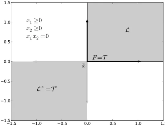
Figure 2– An important feasible set is given by the complementarity conditions, that define the positive axes. In this case the feasible set and the tangent cone coincide, but the linearized cone is the whole positive orthant. Even thoughLproperly containsT, both cones have the same polars.
Figure 3– Abadie holds, that isL=T.
the functional description of the feasible set. We are particularly interested in constraint quali-fications that are associated to the convergence of optimization algorithms and that involve the notion of constant rank of a set of active gradients [11, 35, 26, 39, 37, 8, 9].
3 CONE DECOMPOSITION AND CLASSICAL CONSTRAINTS QUALIFICATIONS
LetC⊂Rnbe a closed convex cone. One of its most important geometric properties is whether C contains a line (passing through the origin) or is composed only of half-lines. Since C is convex, this is equivalent to ask if the origin is an extreme point of C or whether the largest subspace contained inCis just the origin. If the answer to any of the three last questions is yes, thenC is called apointedcone. In this sense studying the largest subspace contained in a cone is important to better understand its geometric properties. This subspace is called the lineality space ofCand can be defined as
L(C)de f= {d ∈C| −d ∈C},
see [12].
Now, let us turn our attention to the polar of the linearized cone that appears in the KKT condi-tions, that is to
L◦=
⎧ ⎨
⎩
d |d = i∈I
λi∇fi(x)¯ +
j∈A(x¯)
µj∇fj(x), µ¯ j ≥0
⎫ ⎬
⎭
.
It is clear from the expression above that the lineality space ofL◦contains at least the subspace
spanned by the equalities gradients. HenceL◦can only be pointed if there are no equality
con-straints. Actually we may argue thatL(L◦)is expected to be exactly this subspace, as equalities
are associated to multipliers that are free of sign. For example, consider the interpretation of the KKT conditions as an equilibrium with the active constraints reacting against minus the gradient of the objective function. Letkbe the index of an active constraint such that both±∇fk(x)¯ ∈L◦. Then this constraint can react against any movement with a component in∇fk(x¯)direction, act-ing like a track that only allow movements in its tangent space. It seems to act as an equality.
Now, using the polyhedral representation ofL◦, it is easy to compute its lineality space. In fact,
let us define
I′de f= {i ∈I∪A(x)¯ | −∇f
i(x)¯ ∈L◦},
then
L(L◦)=span{∇fi(x)¯ |i ∈I′}. (5)
In particular, I′ contains the indexes of all equalities. It may also contain the index of some
inequality constraints, the ones with index in
J−
de f
= {j ∈A(x¯)| −∇fi(x)¯ ∈L◦}. (6)
Moreover, definingJ+
de f
= A(x)¯ \J−, the indexes of all inequalities whose gradients do not
belong to the lineality space, we can decomposeL◦as a (direct) sum of the form
L◦=
i∈I′
λi∇fi(x)¯ |λi ∈R,i ∈I′
+ ⎧ ⎨ ⎩
j∈J+
µj∇fj(x)¯ |µj ≥0, j∈J+ ⎫ ⎬
⎭
. (7)
The first term is a subspace, the lineality spaceL(L◦), and the second a pointed cone.
We can learn a lot about the basic shape of the coneLby analyzing the decomposition above and identifying the dimensions of the subspace and pointed cone components. For example inR2the basic shapes of all possible cones are:
• A single point. The subspace component and the pointed cone are only the origin, that is both have zero dimension.
• A ray. The subspace component is of dimension 0 and the pointed cone of dimension 1.
• A line. Now the subspace component is of dimension 1 and the pointed cone of dimen-sion 0.
• An angle. The subspace component has dimension 0 and the pointed cone, dimension 2.
• A semi-plane. The subspace has dimension one and the pointed cone has dimension 1 or 2 (pointing to the same side of the subspace).
• The whole plane. The subspace component has dimension 2 and the pointed cone dimen-sion 0.
One of the main points of this contribution is to show that many constraint qualifications can be better understood taking into consideration this cone decomposition. Actually, we will show that a whole family of CQs is directly or indirectly trying to ensure that locally the decomposi-tion is stable, at least from the point of view of the dimensions involved. With this aim, let us start with the two most important constraint qualifications, linear independence (regularity) and Mangasarian-Fromovitz CQ.
Definition 3.1. The linear independence constraint qualification, or regularity condition, holds atx if the gradients of all active constraints at¯ x are linearly independent.¯
In this case the index set of the subspace componentI′ is simplyI, as showing that j ∈ J −
directly shows that∇fj(x)¯ can be written in terms of the other active gradients. Moreover, since linear independence is a property that is preserved locally we can see that the local version ofL◦
L◦(x)de f= ⎧ ⎨
⎩
d |d = i∈I
λi∇fi(x)+
j∈A(x¯)
µj∇fj(x), µj ≥0
⎫ ⎬
⎭
still has linearly independent generators for both the subspace component and the pointed cone. That it, it still have the same basic shape asL◦(x)¯ =L◦.
Next we introduce the Mangasarian-Fromovitz constraint qualification (MFCQ) [35] using the notion of positive linear independence.
Definition 3.2.Let V =(v1, v2, . . . , vk)be a tuple of vectors inRnandI¯,J¯index sets such that ¯
I∪ ¯J= {1,2, . . . ,k}. Apositive combinationof elements of V with respect to the (ordered) pair (I¯,J¯)is a vector in the form
i∈ ¯I λivi+
j∈ ¯J
µjvj, µj ≥0,∀j ∈ ¯J.
The tuple V is said to be positively linearly independent (PLI) if the only way to write the zero vector using positive combinations is using zeros coefficients. Otherwise the vectors are said to be positive linear dependent (PLD).
Now we are ready to state MFCQ. Actually, we use an alternative definition that can be found in [41]. The original definition has a stronger geometric flavor but is not well suited for our discussion.
Definition 3.3. The Mangasarian-Fromovitz constraint qualification (MFCQ) holds atx if the¯ set of gradients of all active constraints atx is PLI with respect to¯ (I,A(x)).¯
Once again, it is easy to see that the MFCQ implies that the index set of the subspace component ofL◦is simply the index set of all equalities. In fact, to say that an active inequality gradient is
inL(L◦)is to say that the gradients are PLD. Hence, Mangasarian-Fromovitz CQ is asking that
the natural decomposition of the cone is given precisely by the division of the constraints among equalities and inequalities, that isI′ =I,J
− = ∅, andJ+ =A(x). Moreover, it also requires
that the subspace component have the same dimension around x¯, as it is spanned by linearly independent vectors, therefore preserving its geometric structure locally.
Finally, an interesting remark is that the gradients in the definition of the pointed cone, the gra-dients with index in J+, are always PLI. Hence, their dimension and basic direction will be
preserved locally without further assumptions as positive linear independence is preserved locally by continuous transformations just like the usual linear independence.
4 CONSTANT RANK CONSTRAINT QUALIFICATIONS AND BEYOND
After the discussion above, it starts to become clear that a key property to ensure the validity of a constraint qualification is that the geometric structure of L◦ should be preserved around
¯
x. Moreover, we have learned that this is somewhat summarized by the dimension of its sub-space componentL(L◦)or, in other words, the rank of{∇f
The first constant rank condition was introduced by Janin to study the directional derivative of the marginal value function of a perturbed optimization problem [26]. It was then used in the context of optimization problems with equilibrium constraints [32, 42], bilevel optimization [15], variational inequalities [27], and second order conditions [6, 4].
Definition 4.1. The constant rank constraint qualification (CRCQ) holds at x if for all index¯ subsetsK⊂I∪A(x)¯ the set of gradients{∇fk(y)|k∈K}has the same rank locally around
¯ x .
It is clear from the definition that CRCQ is a generalization of regularity since linear indepen-dence of a group of vectors also imply linear indepenindepen-dence of all its subgroups. Moreover, linear independence of continuous gradients is stable locally,i.e.if it holds atx¯it holds in a neighbor-hood ofx¯. This last fact helps to explain why the definition above asks for a property to hold close tox¯and not only atx¯. In effect, any constraint qualification will need to imply Guignard’s condition that equates the pointwise objectL◦with the geometric objectT◦. SinceT◦depends
on all feasible points close to x¯, it is natural that any constraint qualifications should require, implicitly or explicitly, properties locally aroundx¯.
CRCQ also implies that the index setJ− will remain constant in a neighborhood ofx¯, as the
signs of the positive combinations will be preserved by continuity. Hence, the subspace com-ponent of the local perturbation of the polar of the linearized coneL◦(x)
will be spanned by gradients with the same indexes as inL◦and its geometry will be preserved due to rank
preser-vation.
The constant rank condition was then generalized by taking into account that the multipliers associated to inequality constraints are always positive, similarly to the way MFCQ generalizes regularity. In 2000, Qi and Wei introduced the notion of constant positive linear dependence [39] that was proved to be a constraint qualification in [5].
Definition 4.2. The constant positive linear dependence (CPLD) constraint qualification holds atx if, for all subsets¯ I¯⊂IandJ¯⊂J, the positive linear dependence with respect to(I¯,J¯)of the gradients{∇fk|k∈ ¯I∪ ¯J}imply that they remain PLD in a neighborhood ofx .¯
This condition proved to be very useful in the convergence analysis of optimization algorithms like SQP [39], exterior penalty and augmented Lagrangian methods [3, 2], and inexact restora-tion [17]. It was also generalized to problems with complementarity and vanishing constraints [23, 24].
Again, CPLD implies that the indexes inJ−are stable close tox¯ and hence the subspace
com-ponent ofL◦(x)is generated by gradients with the same indexes as in x¯. The index sets in the
cone decomposition are stable. Moreover, it can be shown that it also implies that the rank of the subspace component is constant close tox¯. We will give more details on this fact below when we define the relaxed version of CPLD.
equalities. Actually, for equality constrained problems it was already known that the constant rank of thefull setof gradients was sufficient to qualify the constraints [4]. Later on, Minchenko and Stakhovski incorporated inequality constraints [37].
Definition 4.3. The relaxed constant rank constraint qualification (RCR) holds at x if for all¯ index sets sets in the formK=I∪ ¯J, where J¯⊂A(x), the set of gradients¯ {∇fk(y)|k∈K}
has the same rank locally aroundx.¯
In [37], the authors showed that RCR implies the existence of a local error bound, that is that it is possible to estimate the distance to the feasible set by using a natural infeasibility measure which is in turn a constraint qualification [43]. They also showed that the error bound property holds under CPLD. A follow up work also used RCR to study the directional differentiability of the optimal value function of a perturbed problem and second order optimality conditions [38].
This condition was then generalized using only positive linear dependence in place of rank by Andreaniet al.in [8].
Definition 4.4. The relaxed constant positive linear dependence constraint qualification (RC-PLD) holds atx if¯
• The gradients of all equality constraints have the same rank in a neighborhood ofx .¯
• LetI¯ ⊂I be the index set of a basis of the space spanned by gradients of all equalities atx. Then, for all¯ J¯ ⊂ A(x)¯ the positive linear dependence with respect to (I,¯ J¯)of {∇fk(x)¯ |k∈ ¯I∪ ¯J}implies that it remains PLD in a neighborhood ofx .¯
This constraint qualification have the same interesting properties as CPLD. It is stable locally, that is if it holds atx¯it holds at all feasible points close to x¯ [8]. It implies the existence of an error bound [8]. It has been used in the context of problems with complementarity constraints and parametric analysis [21, 20, 22, 14], convergence analysis of algorithms [16, 25, 13], and vector optimization [33].
The last two conditions still require properties of gradients whose indexes belong to all possible subsets of active inequalities. We know from the discussion of the previous section that only the active constraints with index inI′, are relevant in the definition of the subspace component of
L◦, see (5) and the following discussion. It is then natural to define a related CQ:
Definition 4.5. The constant rank of the subspace component (CRSC) constraint qualification holds atx if there is a neighborhood of¯ x where the rank of¯ {∇fk(y)|k∈I′}remains constant.
This condition was recently introduced by Andreaniet al.in [9]. An equivalent condition, with an extra, superfluous, assumption, was developed independently by Minchenko and Stakhovski in [36], see also [30].
Among the major properties of feasible sets that conform with CRSC we would like to empha-size the following.
• Under the CRSC, the inequality constraints inJ−hold as equalities for all feasible points
close tox¯. That is, even though those constraints appear only as inequalities in the descrip-tion of the feasible set, the reverse inequality is implied by the other constraints locally. In this sense, the subspace component ofL◦is actually generated only by the equalities that
appear explicitly or implicitly in the description of the feasible set just like in MFCQ.
• The CRSC is stable, that is, if it holds at a feasible pointx¯it holds for all feasible point in a neighborhood ofx¯. This was proved in [9] showing that setJ−is also stable.
• The CRSC implies the error bound property like the previous CQs. The error bound is also in turn a constraint qualification, as it implies Abadie’s CQ [43].
• The convergence theory of many optimization algorithms can be extended from requiring CPLD to just CRSC. This is true at least for methods in the family of pure penalty al-gorithms, multiplier methods, sequential quadratic programming, and inexact restoration. This can be shown using the approximate – KKT sequences [7] and a weaker constraint qualification called constant positive generators (CPG), that can also be used to generalize convergence results for interior points methods. See details in [9].
5 CONCLUSION
We introduced a geometric view of constraints qualifications based on the constant rank condition and showed that their key property is that they preserve the geometric structure of the lineality space of the polar of linearized coneL◦. The weakest condition of this family, called the
con-stant rank of the subspace component (CRSC) still preserves important properties like stability, the validity of an error bound and is adequate to study the convergence of many optimization algorithms like inexact restoration [13] and augmented Lagrangian methods [9].
ACKNOWLEDGMENTS
This work was supported by PRONEX-Optimization (PRONEX-CNPq/FAPERJ E-26/171.510/ 2006-APQ1), CEPID-CeMEAI (FAPESP 2013/07375-0), Fapesp (Grants 2013/05475-7 and 2012/20339-0), CNPq (Grants 305217/2006-2 and 305740/2010-5).
REFERENCES
[1] ABADIEJ. 1967. On the Kuhn-Tucker Theorem. In: J. Abadie, editor,Nonlinear Programming, pages 21–36. John Wiley, New York.
[3] ANDREANIR, BIRGINEG, MARTINEZJM & SCHUVERDTML. 2008. On Augmented Lagrangian Methods with General Lower-Level Constraints.SIAM Journal on Optimization,18(4): 1286–1309.
[4] ANDREANIR, ECHAGUE¨ CE & SCHUVERDTML. 2010. Constant-Rank Condition and Second-Order Constraint Qualification.Journal of Optimization Theory and Applications,146(2): 255–266.
[5] ANDREANIR, MART´INEZJM & SCHUVERDTML. 2005. On the Relation between Constant Posi-tive Linear Dependence Condition and Quasinormality Constraint Qualification.Journal of Optimiza-tion Theory and ApplicaOptimiza-tions,125(2): 473–483.
[6] ANDREANIR, MART´INEZJM & SCHUVERDTML. 2007. On second-order optimality conditions for nonlinear programming.Optimization,56(5-6): 529–542.
[7] ANDREANIR, HAESERG & MART´INEZJM. 2011. On sequential optimality conditions for smooth constrained optimization.Optimization,60(5): 627–641.
[8] ANDREANIR, HAESERG, SCHUVERDTML & SILVAPJS. 2012. A relaxed constant positive linear dependence constraint qualification and applications.Mathematical Programming,135(1-2): 255– 273.
[9] ANDREANIR, HAESERG, SCHUVERDTML & SILVAPJS. 2012. Two New Weak Constraint Qual-ifications and Applications.SIAM Journal on Optimization,22(3): 1109–1135.
[10] BAZARAAMS, SHERALIHD & SHETTYCM. 2006. Nonlinear programming: theory and algo-rithms. John Wiley and Sons.
[11] BERTSEKASDP. 1999. Nonlinear programming. Athena Scientific, Belmont Mass., 2nd ed. edition.
[12] BERTSEKASDP. 2003. Convex analysis and optimization. Athena Scientific.
[13] BUENOLF, FRIEDLANDERA, MART´INEZJM & SOBRALFNC. 2013. Inexact Restoration Method for Derivative-Free Optimization with Smooth Constraints.SIAM Journal on Optimization, 23(2): 1189–1213.
[14] CHIEUNH & LEEGM. 2013. A Relaxed Constant Positive Linear Dependence Constraint Qualifi-cation for Mathematical Programs with Equilibrium Constraints.Journal of Optimization Theory and Applications,158(1): 11–32.
[15] DEMPES. 1992. A necessary and a sufficient optimality condition for bilevel programming problems.
Optimization,25(4): 341–354.
[16] ECKSTEINJ & SILVA PJS. 2013. A practical relative error criterion for augmented Lagrangians.
Mathematical Programming,141: 319–348.
[17] FISCHERA & FRIEDLANDERA. 2010. A new line search inexact restoration approach for nonlinear programming.Computational Optimization and Applications,46(2): 333–346.
[18] GOULDFJ & TOLLEJW. 1971. A Necessary and Sufficient Qualification for Constrained Optimiza-tion.SIAM Journal on Applied Mathematics,20(2): 164–172.
[19] GUIGNARDM. 1969. Generalized Kuhn-Tucker Conditions for Mathematical Programming Prob-lems in a Banach Space.SIAM Journal on Control,7(2): 232–241.
[20] GUOL & LING-H. 2013. Notes on Some Constraint Qualifications for Mathematical Programs with Equilibrium Constraints.Journal of Optimization Theory and Applications,156(3): 600–616.
[22] GUOL, LING-H & YEJJ. 2013. Second-Order Optimality Conditions for Mathematical Programs with Equilibrium Constraints.Journal of Optimization Theory and Applications,158(1): 33–64.
[23] HOHEISELT, KANZOWC & SCHWARTZA. 2012. Convergence of a local regularization approach for mathematical programmes with complementarity or vanishing constraints.Optimization Methods and Software,27(3): 483–512.
[24] HOHEISELT, KANZOWC & SCHWARTZA. 2013. Theoretical and numerical comparison of relax-ation methods for mathematical programs with complementarity constraints.Mathematical Program-ming,137(1-2): 257–288.
[25] IZMAILOVAF, SOLODOVMV & USKOVEI. 2012. Global Convergence of Augmented Lagrangian Methods Applied to Optimization Problems with Degenerate Constraints, Including Problems with Complementarity Constraints.SIAM Journal on Optimization,22(4): 1579–1606.
[26] JANINR. 1984. Directional derivative of the marginal function in nonlinear programming. In Sensitiv-ity, Stability and Parametric Analysis (Mathematical Programming Studies), pages 110–126. Springer Berlin Heidelberg.
[27] JIANGH & RALPH D. 2000. Smooth SQP Methods for Mathematical Programs with Nonlinear Complementarity Constraints.SIAM Journal on Optimization,10(3): 779–808.
[28] JOHNF. 1948. Extremum Problems with Inequalities as Subsidiary Conditions. In: K.O. Friedrichs, O.E. Neugebauer, and J.J. Stoker, editors, Studies and Essays: Courant Anniversary Volume, pages 187–204. Wiley-Interscience, New York.
[29] KARUSHW. 1939. Minima of functions of several variables with inequalities as side constraints. PhD thesis, University of Chicago.
[30] KRUGER AY, MINCHENKO L & OUTRATA JV. 2013. On relaxing the Mangasarian-Fromovitz constraint qualification.Positivity,18(1): 171–189.
[31] KUHNHW & TUCKERAW. 1951. Nonlinear Programming. In: J. Neyman, editor,Proceeding of the Second Berkeley Symposium on Mathematical Statistics and Probability, Berkeley, CA. University of California Press.
[32] LUO Z-Q, PANG JS & RALPH D. 1996. Mathematical Programs with Equilibrium Constraints. Cambridge University Press.
[33] MACIELMC, SANTOSSA & SOTTOSANTOGN. 2012. On Second-Order Optimality Conditions for Vector Optimization: Addendum.Journal of Optimization Theory and Applications.
[34] MANGASARIANOL. 1994. Nonlinear programming. SIAM.
[35] MANGASARIANOL & FROMOVITZS. 1967. The Fritz John necessary optimality conditions in the presence of equality and inequality constraints.Journal of Mathematical Analysis and Applications, 17(1): 37–47.
[36] MINCHENKOL & STAKHOVSKIS. 2010. About generalizing the Mangasarian-Fromovitz regularity condition (in Russian).Doklady BGUIR,8: 104–109.
[37] MINCHENKOL & STAKHOVSKIS. 2011. On relaxed constant rank regularity condition in mathe-matical programming.Optimization,60(4): 429–440.
[39] QIL & WEIZ. 2000. On the Constant Positive Linear Dependence Condition and Its Application to SQP Methods.SIAM Journal on Optimization,10(4): 963–981.
[40] REAYJR. 1966. Unique Minimal Representations with Positive Bases.The American Mathematical Monthly,73(3): 253–261.
[41] ROCKAFELLARRT. 1993. Lagrange Multipliers and Optimality.SIAM Review,35(2): 183–238.
[42] SCHOLTESS & STOHR¨ M. 1999. Exact Penalization of Mathematical Programs with Equilibrium Constraints.SIAM Journal on Control and Optimization,37(2): 617–652.
[43] SOLODOV MV. 2010. Constraint qualifications. In: COCHRANJJ, COX LA, KESKINOCAKP,