Monolayer phosphorene under time-dependent magnetic ﬁeld

(1)

Monolayer phosphorene under time-dependent magnetic

_ﬁ

eld

J.P.G. Nascimento

*

, V. Aguiar, I. Guedes

Departamento de Física, Universidade Federal do Ceara, Campus do PICI, Caixa Postal 6030, 60455-760, Fortaleza, CE, Brazil

A R T I C L E I N F O

Keywords:

Phosphorene Time-dependent systems Lewis and Riesenfeld method Landau level

Quantum-mechanical energy expectation values Probability transition

A B S T R A C T

We obtain the exact wave function of a monolayer phosphorene under a low-intensity time-dependent magnetic field using the dynamical invariant method. We calculate the quantum-mechanical energy expectation value and the transition probability for a constant and an oscillatory magneticfield. For the former we observe that the Landau level energy varies linearly with the quantum numbersnandmand the magneticfield intensityB0:No transition takes place. For the latter, we observe that the energy oscillates in time, increasing linearly with the Landau levelnandmand nonlinearly with the magneticfield. Theðk;lÞ→_ð_n;m_Þ_{transitions take place only for}_l_¼ m:We investigate theð0;0Þ→_ð_n;0Þandð1;lÞandð2;lÞprobability transitions.

1. Introduction

Since the production of graphene in 2004[1]the properties of single and few layers of two-dimensional (2D) materials have attracted great attention owing to possible applications in nanoelectronics. Along the last decade several single layer crystals were also developed as silicene[2], germanene[3], stannene[4], and the transition-metal dichalcogenides[5]. Recently, phosphorene, a single layer of Black Phosphorus[6]has been extensively studied. Due to its high anisotropy, phosphorene ex-hibits interesting direction-dependent optical and transport properties. Investigations on the energy gap and electronic dispersion of different phosphorene materials can be readily found in Refs.[7–_15]_.

In 2015 Zhou et al.[16]investigated theoretically the Landau levels and magneto-transport properties of a monolayer phosphorene under a perpendicular static magnetic ﬁeld. By considering B¼B0k and the

Landau gaugeA¼ Byi; they showed that for low-intensityﬁelds the energy of conduction and valence bands varies linearly with the Landau level indexn and the magneticﬁeldB0:The Landau splittings of the

conduction and valence bands and the respective wavefunctions are different due to the anisotropic effective masses. They also considered the symmetry gauge A¼ ðAx;AyÞand obtained the wave functions in

terms of Laguerre polynomials.

Also in 2015, Zhou et al. [17] studied the Landau levels and magneto-optical conductivity of black phosphorus thinﬁlms under a perpendicular magneticﬁeld based on an effectivek.pHamiltonian and linear response theory. They also studied the effects of interband and intraband couplings by using the time-independent perturbation theory and numerical calculations.

Here we calculate analytically the expressions for the energy and probability transitions of a monolayer phosphorene in the presence of low-intensity time-dependent magneticﬁeld. We use the same Hamil-tonian as in Ref.[16]withB¼BðtÞ; the symmetry gauge and the Lewis and Riesenfeld method[18]to obtain the exact analytical solution of the time-dependent Schr€odinger equation. We obtain the expressions for the mechanical energy average values and probability transitions between Landau levels. We investigate the cases BðtÞ ¼B0k and BðtÞ ¼ ðB2

0þB21cos2ðνtÞÞ 1=2

k:This paper is outlined as follows. In Section2, we calculate the time-dependent wave functions of phosphorene. In Section

3, we obtain the mechanical energy average values and probability transitions for the constant and oscillating magneticﬁeld. Finally, the concluding remarks are presented in Section4.

2. Eigenfunctions of a single-layer phosphorene in the presence of an external low-intensity magneticﬁeld

The time-dependent Schr€odinger equation of a single-layer phos-phorene in the presence of an external low-intensity magneticﬁeld is given by

iℏ∂tΨ_¼_H_Ψ_; ₍₁₎

whereΨ_{¼ ½}_ψc_ψvT

is a two-component spinor, withψc;v_{corresponding}

to the envelope functions associated with the probability amplitudes at the respective sublattice sites (the superscriptTdenotes the transpose of the½…_{vector), and}

* Corresponding author.

E-mail address:joaopedro@ﬁsica.ufc.br(J.P.G. Nascimento).

Contents lists available atScienceDirect

Physica B: Condensed Matter

journal homepage:www.elsevier.com/locate/physb

https://doi.org/10.1016/j.physb.2017.11.089

Received 28 September 2017; Received in revised form 24 November 2017; Accepted 27 November 2017 Available online 5 December 2017

(2)

H¼ 0 B B B @

Ecþ

1

2

₁

m0cx

π2 xþ 1 mcy π2 y 0

0 _E_v 1

2 ₁ m0 vx π2 xþ 1 mvy π2 y 1 C C C A ; (2)

is the Hamiltonian of the system,π¼ ðπ_x;π_yÞ ¼ ðp_x eA_x;p_y eA_yÞis

the generalized momentum,eis the elementary charge,A¼ ðAx;AyÞis

the magnetic vector potential, m0

cx;mcy;m0vx and mvy are effective

masses related to the free electron mass meðm0cx¼0:167me;mcy¼

0:848me;m0vx¼0:184meandmvy¼1:142meÞ and Ec¼0:34eVðEv¼

1:18eVÞis the conduction (valence) band edge.

From Eq. (1) we obtain the following uncoupled differential equations

iℏ_∂t_ψc

ðx;y;tÞ Ecψcðx;y;tÞ ¼

1 2 ₁ m0 cx π2 xþ 1 mcy π2 y ψc

ðx;y;tÞ; (3a)

iℏ_∂t_ψv

ðx;y;tÞ Evψvðx;y;tÞ ¼

1 2 ₁ m0 vx π2 xþ 1 mvy π2 y ψv

ðx;y;tÞ: (3b)

By considering BðtÞ ¼ ð0;0;BðtÞÞ; choosing the gauge Aðr;tÞ ¼ ð1=2ÞrBðtÞ; and rediﬁng the cartesian coordinates as x¼ ðmcy=m0cxÞ

1=4

X andy¼ ðm0

cx=mcyÞ1=4YEq.(3a)reads

ðiℏ∂t _E_c_Þψc

ðX;Y;tÞ ¼

1

2_M_c

P2

XþP

2 Y

ωcðtÞ

2 ~Lz

þMcω 2 1cðtÞ

2

X2

þY2

ψc_ð_X;_Y;_t_Þ_;

(4)

where PX¼ iℏ∂=∂X;PY¼ iℏ∂=∂Y;Mc¼

ffiffiffiffiffiffiffiffiffiffiffiffiffiffiffi

m0

cxmcy

p

;ωcðtÞ ¼eBðtÞ=Mc; ~

Lz¼XPY YPX;andω21cðtÞ ¼e2B2ðtÞ=4Mc2:

By applying the unitary transformation

ψc_ð_X;_Y;_t_{Þ ¼}_U

1φcðX;Y;tÞ ¼exp

i

1

2ℏL~z∫ωcðtÞdt Ec

ℏt

φc_ð_X;_Y;_t_Þ_;

(5)

we can map Eq.(4)into that of a two-dimensional harmonic oscillator with time-dependent frequency, namely

iℏ∂tφc_ð_X;_Y;_t_{Þ ¼}

1

2_M_c

P2

XþP

2 Y

þMcω

2 1cðtÞ

2

X2

þY2

φc_ð_X;_Y;_t_Þ_: ₍₆₎

Lewis and Riesenfeld showed that an invariant for Eq.(6)is given by Ref.[18]

IðtÞ ¼1

2 " X ρ_c 2 þ Y ρ_c 2

þ ðρcPX Mcρ_cXÞ 2

þ ðρcPY Mcρ_cYÞ 2

#

; (7)

whereρ_cðtÞsatisﬁes the generalized Milne-Pinney[19,20]equation

€

ρ_cþω2 1cðtÞρc¼

1 M2 cρ 3 c ; (8)

and only real solutions ofρ_cðtÞare acceptable to haveIhermitian. According to Lewis and Riesenfeld[18], the invariantIðtÞis supposed to satisfy the eigenvalue equation

Iϕn;mðX;Y;tÞ ¼λn;mϕn;mðX;Y;tÞ; (9)

where λn;m are time-independent discrete eigenvalues and

ϕn;m;ϕn0_;_m0

¼δnn0δ_mm0:The solutions of Eq.(6),φc

n;m; are related to the

eigenfunctionsϕn;mofIby

φc

n;mðX;Y;tÞ ¼exp½iαn;mðtÞϕn;mðX;Y;tÞ; (10)

where the phase functionsαn;mðtÞsatisfy the equation

ℏdαn;mðtÞ dt ¼

ϕn;mðX;Y; tÞ i

ℏ∂

∂t H

0_ð_t_Þ

ϕn;mðX;Y;tÞ

; (11)

andH0_ð_t_Þ_{corresponds to the right-hand side of Eq.}₍₆₎_.

Next, consider the unitary transformation

ϕ0n;mðX;Y;tÞ ¼U2ϕn_;_mðX;Y;tÞ; (12)

where

U2¼exp

iMcρ_c

2ℏρc

X2

þY2

: (13)

Under this transformation and deﬁningX¼ρcrcosθandY¼ρcrsinθ; Eq.(9)now reads

I0_ð_t_Þ_σ

n;mðr;θÞ ¼

_ℏ2

2

∂2 ∂r2þ

1

r

∂ ∂rþ

1

r2 ∂2 ∂θ2

þr

2

σn;mðr;θÞ

¼λn;mσn;mðr;θÞ; (14)

whereI0_ð_t_{Þ ¼}_U

2IðtÞU2y;r2¼X 2_þ_Y2

ρ2

c ;θ¼tan 1 Y X and

ϕ0n;mðX;Y;tÞ ¼

1

ρ_cσn;mðr;θÞ: (15)

We decomposeσðr;θÞin the formσðr;θÞ ¼RðrÞΘ_ð_θ_Þ_; _whereΘ_ð_θ_{Þ ¼} eimθ

;withm 2 ℤ_{. By de}_ﬁ_{ning a new variable}_u_¼r2

ℏand writingσðu;θÞ ¼

RðrÞΘ_ð_θ_Þ_as

σðu;θÞ ¼ ðℏ_u_Þjmj2_e u2_vð_uÞΘ_ð_θ_Þ_; ₍₁₆₎ Eq.(14)becomes

u∂

2

vðuÞ

∂u2 þ ðjmj þ1 uÞ

∂vðuÞ

∂u þ

1

2

λn;m

ℏ jmj 1

vðuÞ ¼0_; ₍₁₇₎

whose solutions are expressed in terms of associated Laguerre poly-nomial

vðuÞ ¼Ljmj

n ðuÞ; (18)

where

n¼1

2

λnm

ℏ jmj 1

; (19)

n2ℕ_and_j_m_j_n:_{Observe that for each}_n;_m_{can assume 2}_n_þ_{1 values.}

The normalized eigenfunctions of the invariantIðtÞread

ϕn;mðX;Y;tÞ ¼

_Γ

ðnþ1_Þ Γ_ð_n_{þ j}_m_{j þ}1_Þ

1

π

1₌2₁

ℏρ2 c jmjþ 1 2 X2

þY2jmj2 eimθ

exp

₁

2ℏρc

₁

ρc

iMcρ_c

X2

þY2

Ljmj

n

X2

þY2

ℏρ2 c

;

(20)

and the time-independent eigenvalues are written as λn;m¼ℏð2nþ

jmj þ1Þ: The phasesαc

n;mðtÞwhich satisfy Eq.(11)are

αc

n;mðtÞ ¼ ð2nþ jmj þ1Þ∫

t 0

dt0 Mcρ2cðt0Þ

: (21)

(3)

ψc n;mðr;tÞ ¼

₁

ℏρ2 c

jmjþ

1

2 _Γ

1

π

12 eiαc

n;mðtÞ_exp

i

m 2∫ωcðtÞdt

Ec ℏt ffiffiffiffiffiffiffi m0 cx mcy s

x2þ

ffiffiffiffiffiffiffi mcy m0 cx r y2 ! jmj 2 exp " 1

2ℏρc

1

ρc

iMcρ_c ffiffiffiffiffiffiffi m0 cx mcy s x2 þ ffiffiffiffiffiffiffi mcy m0 cx r y2 !#

eimθc

r_Ljmj

n "

1

ℏ_ρ2 c ffiffiffiffiffiffiffi m0 cx mcy s x2 þ ffiffiffiffiffiffiffi mcy m0 cx r y2 !# ; (22)

whereθcr¼tan 1

" ffiffiffiffiffiffi mcy m0 cx q _y x #

;n2ℕ_and_j_m_j_n:

The solution of Eq. (3b) is easily obtained by replacing m0

cx→ m0vx;mcy→ mvyandEc→Ev; namely

ψv n;mðr;tÞ ¼

₁

ℏ_ρ2 v

jmjþ

1

2 _Γ

1

π

12 eiαv

n;mðtÞ_exp

i

m 2∫ωvðtÞdt

Ev ℏt ffiffiffiffiffiffiffi m0 vx mvy s x2 þ ffiffiffiffiffiffiffi mvy m0 vx r y2 ! jmj 2 exp " 1

2ℏ_ρ

v

₁

ρv

iMvρ_v ffiffiffiffiffiffiffi m0 vx mvy s x2 þ ffiffiffiffiffiffiffi mvy m0 vx r y2 !#

eimθv

r_Ljmj

n "

1

ℏρ2 v ffiffiffiffiffiffiffi m0 vx mvy s x2 þ ffiffiffiffiffiffiffi mvy m0 vx r y2 !# ; (23)

whereMv¼

ffiffiffiffiffiffiffiffiffiffiffiffiffiffiffi

m0

vxmvy

p

;ωvðtÞ ¼eBðtÞ=Mv;θvr¼tan 1

ffiffiffiffiffiffiffi mvy m0 vx q _y x and αv

n;mðtÞ ¼ ð2nþ jmj þ1Þ∫ t 0

dt0 Mvρ2vðt0Þ

: (24a)

withρvðtÞsatisfying the Milne-Pinney equation

€

ρ_vþω2 1vðtÞρv¼

1 M2 vρ 3 v : (24b)

whereω2

1vðtÞ ¼e2B2ðtÞ=4M2v:For a constant magneticﬁeld Eqs.(22) and (23)agree with those found in Ref.[16].

3. Results and discussion

Using the Cartesian coordinates x as generalized coordinates, the Lagrangian of a particle of massmand chargeqmoving in a electro-magnetic ﬁeld reads L¼ ðm=2Þx_2_þ_q_A_⋅_x _q_ϕ_: _{The magnetic vector}

potentialAand the electric scalar potentialϕare in general functions ofx

andt. According to Ref.[21], the Hamiltonian of this system is the me-chanical energy since the“_potential”_{energy in an electromagnetic}_ﬁ_{eld is} determined only byϕ:In this case, the canonical momentum isp¼mx_þ

qAand the Hamiltonian reads H¼ ðp eAðr;tÞÞ2=2mþqϕ:Thus, from Eqs.(22) and (23)we obtain the following quantum mechanical energy expectation values for conduction and valence electrons

Ec

n;mðtÞ ¼Ecþ

ℏ

2

m0

cxmcy 1=2

ð2_n_{þ j}_m_{j þ}1_Þ

β2

cþ

e2

B2

ðtÞ

4 ρ

2 c

meBðtÞ

;

(25a)

Ev n;mðtÞ ¼Ev

ℏ

2

m0

cxmcy 1₌2

ð2_n_{þ j}_m_{j þ}1_Þ

β2

vþ

e2

B2

ðtÞ

4 ρ

2 v

meBðtÞ

:

(25b)

whereβ2_j ¼1þρ

2 jρ_

2 jMj2

ρ2

j .

Thus, for a givenBðtÞone has to solve Eqs.(8) and (24b)to obtain the mechanical energy En;mðtÞ for electrons and holes in a single-layer

phosphorene. First, consider the static caseBðtÞ ¼B0k:The solutions of

Eqs.(8) and (24b)areρ_c¼ρ_v¼₂

eB0

1=2

and the energy average values

for electrons and holes are given by

Ec

n;m¼Ecþ

ℏ_eB0

m0

cxmcy 1=2

nþjmj mþ1

2

; (26a)

Ev n;m¼Ev

ℏ_eB0

m0

vxmvy 1=2

nþjmj mþ1

2

: (26b)

The Landau level energy varies linearly withn;mandB0:For eachn; the indexmtakes 2nþ1 values. From Eq.(26)and for aﬁxedn;we have two situations to consider. Ifm0; we havenþ1 degenerated states while, form<0; nstates are nondegenerated.

For an oscillating magneticﬁeldBðtÞ ¼ ðB2

k;Eq.(8)

and its solution read, respectively,

€

ρcþ

e2

4_M2 c

B2

0þB

2

1cos 2

ðνtÞ

ρc¼

1 M2 cρ 3 c ; (27a)

ρ_cðtÞ ¼

₁

jWjMc

12

MC2

e2

r 8_M2

cν 2;

e2

B2 1

16_M2 cν

2;νt

þMS2

e2

r 8_M2

cν 2;

e2

B2 1

16_M2

cν

2;νt 12

; (27b)

wherer¼2B2

0þB21;MCandMSare the even and odd Mathieu functions,

respectively, andW is the Wronskian ofMCandMS:InFig. 1we plot Ec

n;0ðtÞ shifted by Ec for some values of n: We observe thatEcn;0ðtÞ

oscillates with the same period of the oscillating magneticfield,T¼π=v; and increases withn:The oscillation reflects the increasing (decreasing) of the magnetic interaction when the magnetic field increases (decreases).

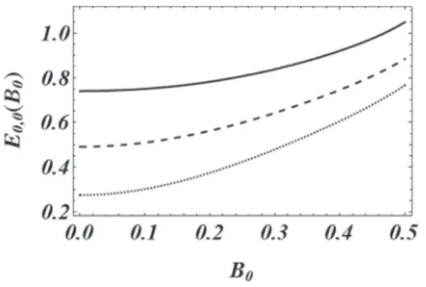
InFig. 2we plotE0;0ðB0Þshifted by Ec;vfor three values oft and

observe thatE0;0ðB0Þdoes not vary linearly withB0:The region deﬁned

by theE0;0ðB0Þ

t¼0andE0;0ðB0Þ

t¼π=2curves deﬁne all possible values of

E0;0ðB0Þ; since the period of oscillation isT¼π:

The probability of transition from an initial stateψj_k_;_lðr;t0Þto another

state ψjn;mðr;tÞ ðt>t0Þ reads Pjðk;lÞ→ðn;mÞðtÞ ¼

R

j

ðk;lÞ→ðn;mÞðtÞ 2

; where

Rjðk;lÞ→ðn;mÞðtÞis the amplitude transitionhn;m;tjk;l;t0i; or

Fig. 1.Plots ofEc

(4)

Rj_ð_k_;_l_Þ→ðn;mÞðtÞ ¼∬ þ∞

∞dxdy

h

ψj n;mðr;tÞ

i*

ψjk;lðr;t0Þ; (28)

wherejiscto conduction band electrons andvto valence band holes. From Eqs. (22) and (23), deﬁning ρ_jðtÞ ¼ρ_j;ρ_jðt0Þ ¼ρ0;j;ρ_jðtÞ ¼ _

ρj;ρ_jðt0Þ ¼ρ_0;j; as well as

a2 jðtÞ ¼

1

ℏρ2 j

; b2 jðt0Þ ¼

1

ℏρ2 0_;j

; (29a)

BjðtÞ ¼iMj

ρ_jρ__ja2

jðtÞ ρ0;jρ_0;jb 2 jðt0Þ

; (29b)

Aj k;l;n;m¼

1

ℏρ2 0_;j

!jljþ21 1

ℏρ2 j

!jmjþ21

Γ_ð_k_þ1_Þ Γ_ð_k_{þ j}_l_{j þ}1_Þ

1

π

12 _Γ

1

π

12 e iαj

n;mðtÞ

eiα

j k;lðt0Þ

exp

i

m 2∫

t 0ωjðt0Þdt0

Ej

ℏt

exp

i

l 2∫

t0

0ωjðt0Þdt0

Ej

ℏt0

;

(29c)

and using X¼r cosðθj_rÞandY¼r sinðθj_rÞ; where X¼ ðmjy=m0jxÞ 1=4

x

andY¼ ðm0

jx=mjyÞ 1=4y; Eq.(28)reads

Rj

ðk;lÞ→ðn;mÞðtÞ ¼δl;mπAjk;l;n;m∫

∞

0 du u

jlj_Ljlj

n h

a2 jðtÞu

i

Ljklj h

b2 jðt0Þu

i

expn u

2

h

BjðtÞ þa 2 jðtÞ þb

2 jðt0Þ

io

; (30)

where u¼r2 _and _Ljlj

nðzÞ are the associated Laguerre polynomials. By

considering the generating functions

X∞

i¼0

siLjilj h

a2 jðtÞu

i

¼ 1 ð1 _s_Þjljþ1exp

a2 jðtÞu

s

ð1 _s_Þ

; ðjsj<1_Þ ₍₃₁₎

and

X∞

β¼0

wβ_Ljlj β

h

b2 jðt0Þu

i

¼ 1 ð1 _w_Þjljþ1exp

b2 jðt0Þu

w

ð1 _w_Þ

; ðjwj<1_Þ ₍₃₂₎

we found after some algebra

Rj_ðk;lÞ→_ðn;mÞðtÞ ¼δl;mπAjk;l;n;m

X k

p¼0 8

> <

> :

ðnþkþ jlj pÞ!

p!ðk pÞ!ðn pÞ!ð 1Þ

p₂jljþ1h

BjðtÞ a 2

jðtÞ b

2 jðt0Þ

ip

h

BjðtÞ a 2 jðtÞ þb

2 jðt0Þ

in ph

BjðtÞ þa 2

jðtÞ b

2 jðt0Þ

ik p

h

BjðtÞ þa2jðtÞ þb 2 jðt0Þ

inþkþjljþ1p

9

> > =

> > ;

;

(33)

indicating that the transitionsðk;lÞ→_ð_n;_m_Þ_{are possible only if}_l_¼_m: Observe that for a static magneticﬁeld the transition probability is Pjðk;lÞ→ðn;mÞðtÞ ¼δl;mδk;nand no transitions are allowed, sinceψjk;lðr;t0Þand

ψjn;mðr;tÞare stationary states. However, forBðtÞ ¼ ðB20þB21cos2ðνtÞÞ 1=2

k

some transitions occur as shown inFig. 3(a) and (b). FromFig. 3(a) we observe that Pc

ð0;0Þ→ðn;0ÞðtÞoscillates withtand fort¼pT¼πp=v; with

p¼0;1;2…_; _{the system will remain in the initial state} _ð₀_;₀_Þ_: _This behavior also reﬂects the oscillation of the magnetic interaction.The probability for transitionsð0;0Þ→_ð_n;₀_Þ_{decreases with increasing}_n_{. In} Fig. 3(b) we plot Pc

ð1;lÞ→ð2;lÞðtÞfor some values ofl:We observe that

Pc

ð1;lÞ→ð2;lÞðtÞis symmetric inland increases with increasingjlj:

4. Concluding remarks

We obtained the wave function of electrons and holes in a monolayer phosphorene in the presence of a low-intensity time-dependent magnetic

ﬁeld. By consideringB¼ BðtÞ; the symmetry gauge and the Lewis and Riesenfeld method the wave functions found for electrons and holes are given by Eqs.(25a) and (25b), respectively. They are expressed in terms of the solutions of the Milne-Pinney equations given by Eqs.(8) and (24b). From the wave functions obtained we calculated the quantum-mechanical energy expectation value and the transition probability for two magneticﬁelds,BðtÞ ¼B0kandBðtÞ ¼ ðB2

k: For a constant magnetic ﬁeld we observe that the

quantum-Fig. 3.Plots of (a)Pc

ð0;0Þ→ðn;0ÞðtÞfor transitionsn¼0 (solid line),n¼1 (dashed line) andn¼2 (dotted line) and (b)Pcð1;lÞ→ð2;lÞðtÞfor transitionsl¼0 (solid line) andl¼ 1 (dashed line).

In thisﬁgure we usedℏ_¼me¼ν¼e¼ 1 andB0¼B1¼0:5:

Fig. 2.Plots ofE0;0ðB0Þfort¼0 (solid line),t¼π=4 (dashed line) andt¼π=2 (dotted

(5)

mechanical energy expectation value scales linearly with the Landau levelsnandmand the magneticﬁeldB0. In this case, the wave functions

are stationary states and no transitions are allowed. For an oscillatory magnetic field we observe that the quantum-mechanical energy expectation value scales linearly with the Landau levels nandm and nonlinearly with the magneticfield. The nonlinear behavior observed with the magneticfield results from the solutions of the Milne-Pinney equations given by the Mathieu functions. The transition probabilities

ð0;0Þ→_ð_n;₀_Þ_{decrease with increasing}_n; _{while those connecting}_ð₁_;_l_Þ andð2;lÞincreases with increasingl.

Acknowledgments

The authors are grateful to the National Counsel of Scientiﬁc and Technological Development (CNPq) of Brazil forﬁnancial support.

References

[1] A.E. Bragg, J.R.R. Verlet, A. Kammrath, O. Cheshnovsky, D.M. Neumark, Science 306 (5696) (2004) 666.

[2] B. Lalmi, H. Oughaddou, H. Enriquez, A. Kara, S. Vizzini, B. Ealet, B. Aufray, Appl. Phys. Lett. 97 (2010), 223109.

[3] M.E. Davila, L. Xian, S. Cahangirov, A. Rubio, G. Le Lay, New J. Phys. 16 (2014), 095002.

[4] S. Saxena, R.P. Chaudhary, S. Shukla, Sci. Rep. 6 (2016) 31073.

[5] D. Xiao, G.-B. Liu, W. Feng, X. Xu, W. Yao, Phys. Rev. Lett. 108 (2012), 196802. [6] X. Liu, J.D. Wood, K.-S. Chen, E. Cho, M.C. Hersam, J. Phys. Chem. Lett. 6 (2015)

773.

[7] Y. Takao, H. Asahina, A. Morita, J. Phys. Soc. Jpn. 50 (1981) 3362. [8] A. Morita, Appl. Phys. A 39 (1986) 227.

[9] X. Peng, Q. Wei, A. Copple, Phys. Rev. B 90 (2014), 085402.

[10] A.S. Rodin, A. Carvalho, A.H. Castro Neto, Phys. Rev. Lett. 112 (2014), 176801. [11] R. Fei, V. Tran, L. Yang, Phys. Rev. B 91 (2015), 195319.

[12] J. Dai, X.C. Zeng, J. Phys. Chem. Lett. 5 (2014) 1289.

[13] H. Guo, N. Lu, J. Dai, X. Wu, X.C. Zeng, J. Phys. Chem. C 118 (25) (2014) 14051. [14] D.J.P. de Sousa, L.V. de Castro, D.R. da Costa, J. Milton Pereira Jr., Phys. Rev. B 94

(2016), 235415.

[15] G.O. de Sousa, D.R. da Costa, Andrey Chaves, G.A. Farias, F.M. Peeters, Phys. Rev. B 95 (2017), 205414.

[16] X.Y. Zhou, R. Zhang, J.P. Sun, Y.L. Zou, D. Zhang, W.K. Lou, F. Cheng, G.H. Zhou, F. Zhai, Kai Chang, Sci. Rep. 5 (2015) 12295.

[17] X. Zhou, W.-K. Lou, F. Zhai, K. Chang, Phys. Rev. B 92 (2015), 165405. [18] H.R. Lewis Jr., W.B. Riesenfeld, J. Math. Phys. 10 (1969) 1458. [19] W.E. Milne, J. Res. Natl. Bur. Stand. 43 (1949) 537. [20] E. Pinney, Proc. Am. Math. Soc. 1 (1950) 681.