A Work Project, presented as part of the requirements for the Award of a Master Degree in Economics from the NOVA – School of Business and Economics
Wage Inequality, Productivity, Peer Effects and Assortative
Matching
Ana Margarida Neves de Carvalho Student Number 795
A Project carried out on the Master in Economics Program, under the supervision of: Professor Pedro Portugal
Wage Inequality, Productivity, Peer Effects and Assortative
Matching
Abstract
Using a remarkable matched employer-employee dataset, this thesis investigates how wage dispersion evolved in Portugal and whose components contributed more to this variation, highlighting the impact of peer effects in both individual wages and wage inequality. A re-gression model with high dimensional fixed effects is used. The results show that, contrary to the case of Germany, wage dispersion in Portugal has decreased over the last decade. Person effects are the main contributors, with its contribution rising over time, contrasting with the declining role of firm effects. The role of peer effects in wage dispersion ranges between 4.2% and 6.6%, with a one standard deviation increase impacting on individual wages with that same magnitude.
Keywords: Wage Dispersion, Peer Effect, High Dimensional Fixed Effects, Variance Decomposition
1 Introduction
Firm heterogeneity has been found to play an important role in explaining wage dispersion. Consequently, shedding light on how one important intrinsic characteristic of firms, the quality of their workforce, is pertinent departing, at the same time, from the usual attribution of variation to different wage posting and/or wage bargaining policies. Indeed, Battisti (2013) found that the quality of the co-workers of an individual worker contributes to wage dispersion while, simultaneously, reducing the contribution of the firm component.
productivities by virtue of an improved performance of a worker after his interaction with a more productive co-worker. Hence, this consists on a reason for the existence of firms. If peer effects are negligible, this reason will not be in force. Therefore, and in accordance with Bloom et al. (2015), people could be more productive when working from home than when they work in a physical establishment, interacting with their peers.
This thesis intends to unravel the extent to which peer effects are relevant in the Portuguese labor market and whether they influence wage dispersion, the latter inserted in the broader picture of figuring out which components contribute more to wage inequality. It aims to provide new insights on wage inequality in Portugal, since most of the research done up to this point only covers the period until the end of the XX century.
The remaining sections of this paper are organized in the following way: section 2 consists on an overview of the literature related with this study; section 3 gives a brief synopsis of past research on wage dispersion in Portugal; sections 4 and 5 lay out the empirical methodology of the research and the characteristics of the data, respectively; section 6 provides the key findings on the role of peer effects and its impact on inequality, while section 7 concludes.
2 Literature Review
Wage inequality has received consideration due to its increase in many countries. Previous studies have identified demand-side (technological change and alterations in the trade pattern resulting from a more integrated world economy) and supply-side (increase in the relative supply of high-education workers) explanations, along with labour market institutional changes (the re-duction of union density or the evolution of minimum wage legislation) as possible explanations for this trend, as stressed in Dunne et al. (2000) and Faggio, Salvanes, and Reenen (2007).
portable skills and the one from firms’ pay premiums that impact wage inequality. They find that the exacerbation of wage inequality was driven by an increasing dispersion of the worker-specific component of pay, along with the employer-worker-specific component and an increase of their covariance, indicating an increment of positive assortative matching.
The pervasiveness of firm specific wage premiums in the labour market leads to an unmistakable relevance of the study of its impact on wage differentials, notably concentrating on the effect of employer characteristics on wages. Groshen (1991) reported their importance using US data for intra-industry wage differentials whereas Card, Cardoso, and Kline (2016) demonstrate their importance for the gender wage gap using Portuguese data. Rent-sharing, strategic wage posting behaviour, efficiency wage premiums and compensating differentials are explanations given to the existence of firm specific wage premiums. Card et al. (2016) look at the firm switching literature (which propounds that gains or losses in wages due to workers changing firms can be anticipated) and reconciled it with rent-sharing estimates obtained through the study of how firm productivity impacts workers’ wages. Hence, it is possible to connect rent-sharing elasticities with wage inequality. As a matter of fact, if we observe either increasing differences on produc-tivity or rising differences in the share of rents that employees obtain at diverse workplaces, then we are able to explain part of the increase in wage inequality. Alternatively, one could focus on models of imperfect competition of the labour market, taking into account the market power of firms arising from the different valuations that workers’ exhibit of job amenities. Under those circumstances, search frictions are not necessary for firms to have some monopsony power in setting wages. Furthermore, Van Reenen (1996) studies quasi-rents’ sharing arisen from break-through innovations, where he finds that although technological change increases average firm wages, it does not seem to influence the shape of the wage structure. Notwithstanding this result, it does not exclude the possibility of technological diffusion having an effect on wage inequal-ity, through, for instance, the increase of demand for high skilled workers to face the spread of new technologies, as predicted by the skill-biased technical change argument in Davis and Haltiwanger (1991).
of an individual leads to a decline on the part of wage variation explained by firm effects. Ac-cordingly, the composition of a firm’s workforce seems to be a prominent component of the effect that firms’ characteristics have on wages. On that account, it is pertinent to determine the extent to which employees’ quality drives firm heterogeneity. This reasoning derives from the possible existence of technological spillovers, which refer to the productivity-enhancing ex-change of knowledge accruing from interactions among employees. The conceivable increment of spillovers is of concern to the enlargement of wage inequality, as it could result in increasing productivity differences among firms. As a matter of fact, Cornelissen, Dustmann, and Schön-berg (2013) stress that the existence of peer effects may give rise to a larger long-term inequality if high skilled workers gather in the same peer groups.
Although peer effects are originally considered in an education setting, evidence on their exis-tence at the workplace began with studies on specific occupations, which take the form of real data on a single firm or occupation (for example, Mas and Moretti (2009) focus on the existing peer effect in a supermarket chain, providing evidence on the prevalence of peer pressure) or of a laboratory experiment. In light of the need to determine whether extrapolation of these findings to the labor market as a whole is possible, Cornelissen, Dustmann, and Schönberg (2013) focus on this issue while considering the impact peer effects have on wages instead of on productivity. The authors identify “peer pressure” as one way through which the productivity of one worker is enhanced by another, since falling short of what a peer has achieved may trigger a larger effort from the part of the worker. On the other hand, there may exist “knowledge spillovers” whereby communication among workers leads to the development or improvement of skills that would not occur otherwise.1 These factors entail that workers have a higher productivity when their
co-workers’ productivity is high.
In contrast to these arguments, Mas and Moretti (2009) enunciate the case where co-workers may engage in free-riding if the output of each worker is not completely observable, which turns out to be burdensome if the employer wants to reward high effort. Moreover, as suggested in Kremer (1993), if different workers have a different amount of human capital, a “skills incompatibility” 1An example, for the Portuguese case, is Martins and Jin (2010) that develop a learning model in which an
problem may arise, implying that firms with a uniform labor force in terms of human capital will have a higher productivity.
Setting his sights on determining how the quality of a worker’s peers impact his wage, Battisti (2013) identifies, besides the presence of peer pressure, the existence of complementarities in the production function of each individual to be one of the reasons why the degree of skills of a co-worker matter for his wage, since the marginal productivity of each person will depend on peer quality. Furthermore, the wage of a worker may be influenced by his reservation wage, which, in turn, might depend on the groups of co-workers. To put it differently, an individual may accept a lower wage when he has the opportunity to work alongside a peer group that he prefers. This is a compensating differential rationale, entailing a wage reduction since an amenity – working with preferred co-workers – exists. It is not possible to disentangle whether, in this context, the spillover effect is positive or negative. Lastly, bargaining externalities are a factor to consider in this setting. In case bargaining outcomes are positively correlated in a workplace, the extraction of higher shares of surplus by high quality individuals will bring about an increase in wages of peers. Therefore, having high skilled peers will increment a worker’s wage. However, if wages are a fixed share of revenues and some groups comprise a larger bargaining power than the remaining, this effect may be negative.
3 Wage Inequality in Portugal
Most existing studies on wage inequality in Portugal concern the late 80’s and early 90’s. In Cardoso (1997), Cardoso (1998) and Cardoso (1999), wage inequality in Portugal is the topic under study. Having as a benchmark the period between 1983 and 1992, it is observed that inequality in the labour market verified an upward trend. This growth was mainly due to an increasingly stretched upper half of the wage distribution. The share of inequality originating from worker characteristics was found to increase, mainly due to a sharp increment of returns to schooling in high-paying firms. Furthermore, rising inequality was found to be generated by changes in the employment structure, through the rise in the demand for more qualified workers taking place within industries. Nevertheless, firms seemed to be valuing less labour market experience and age, as progression mechanisms based on seniority diminished from 1983 to 1992. Modernization of the economy is usually appointed as the driving force stimulating the upgrade of the quality of employees, which is accompanied by the observed increase in the returns to education. On balance, inequality in the aforementioned period derives from high wages being very high when compared to the remaining distribution. The Portuguese wage distribution was, therefore, characterized by a compressed bottom and a stretched top. The fact that education returns are higher for highly paid jobs, impacting positively on wage dispersion, is also verified in Machado and Mata (2001).2 These authors find tenure to have more influence
at lower paid jobs, larger firms to pay more to all workers and that firms with foreign capital increase wages more to those in higher paid jobs.
In Cardoso (2004), the Portuguese case is contrasted with the one of the UK: while in the latter wage inequality verified an uninterrupted positive trend, in the former there seems to be a turning point as inequality is found to be decreasing in the period 1994-1999. There is a relatively small body of literature that analyses a more recent period.
Provided that wage dispersion has not been extensively studied for the Portuguese case, it is relevant to disentangle the contribution that worker, firm and peer components have been having 2They verify that the tendency sharpens between 1982 and 1994. Hence, the rising returns to education coincide
in shaping it, while simultaneously comparing the results to what has been witnessed in other countries.
4 Empirical Framework
4.1 Baseline wage regression and inclusion of spillovers
The methodological approach used in this study rests on the econometric framework developed by Card, Heining, and Kline (2013), which intents on unravelling the extent to which individual-specific or firm-individual-specific characteristics impact on wage dispersion. Under those circumstances, we are going to rely on the following equation, which is designated as the AKM model, specified in Abowd, Kramarz, and Margolis (1994):
yit =αi +θJ(i,t)+x
′
itβ+ϵit , (1)
whereyitis the logarithm of the real hourly wage for worker i at year t;x′itconsists on a vector
of observed time-varying characteristics of workers along with a set of year dummies;3 α
i is a time-invariant worker fixed effect, meaning it encompasses worker-specific characteristics that are rewarded equally by firms; θJ(i,t) is a time-invariant establishment fixed effect, consisting
on the proportional pay premium given by firm j to all workers; andϵitis the disturbance term of the regression, which follows the conventional assumptions (zero mean, strict exogeneity).
An objective of this study is to investigate how the wage structure has changed over the course of the years. With this intention, intervals of seven years will be considered. In each of these intervals separate linear models will be fitted, as done in Card, Heining, and Kline (2013). This procedure entails the usage of high-dimensional fixed effects, whereby estimation by the usual OLS formula is hindered, since the dimension of the matrices for the fixed effects render it un-feasible to use the formerly specified formula. Acknowledging this limitation, we resort to an
3In our case, it includes the following observed time varying characteristics of employees: age, age squared,
algorithm developed by Guimarães and Portugal (2010) to circumvent the problem.4
Conse-quently, we are able to solveminα,θ,β∑i∑t
[
yit−αi−θJ(i,t)−x
′ itβ
]2. One point that should
not be overlooked concerns the identification of the worker and firm fixed effects. Thereupon, identification is achieved by considering the largest connected set of observations. In other words, firms are linked by worker mobility, so that as workers move from firm to firm, we are able to disentangle the fixed effect of that firm, enabling us to further determine the worker fixed effect because, after knowing and accounting for the one correspondent to the firm, the remain-ing differences in pay would result from worker-specific characteristics. Henceforth, there is the widespread need of relying on a connected set to have identifiable employer and employee fixed effects.5
On the other hand, departing from the research in which our base model hinges on, we will focus on the contribution of co-workers’ characteristics towards the wage of an individual. Accord-ingly, we resort to Arcidiacono et al. (2012) by constructing a spillover effect consisting on the linear combination of individual fixed effects. Hence, the model to be estimated is:
yit =αi+θJ(i,t)+x
′
itβ+γα−i+ϵit, (2)
where α−i = Nijt1 ∼i
∑
k∈N ijt∼i
αk is the mean of the person fixed effects of the co-workers of worker i (is gauged without including worker i) andγis its coefficient (the impact that the peer
effect has on the logarithm of an individual i’s real hourly wage).6 In this setting, the co-workers
of worker i are all workers that, in a given year, are in the same firm as i.7 There is the need to
4This consists on an iterative gradient algorithm. In the context ofY = A
1α+A2θ+Bβ+ϵ, we obtain the
following matrix:
α= (A′1A1)−1A′
1(Y −A2θ−Bβ) θ= (A′2A2)−1A
′
2(Y −A1α−Bβ) β = (B′B)−1B′
(Y −A1α−A2θ)
.
We are able to solve it by alternating between the estimation ofβandαandθ, without having to worry about the dimensionality ofA1andA2, avoiding inversion of large matrixes by estimatingβfirst and then adding the fixed effect components as additional covariates. The estimation procedure converges, attributing the value of 1 to the coefficients ofA1αandA2θ. Therefore, the estimation is done on a first stage by giving starting values for α′sandθ′sand, conditional on them, estimating the coefficients of the explanatory variables; subsequently, we
take the former values as given and re-estimateα′sandθ′s; this process goes on until convergence is achieved.
This is possible by virtue of the decline of the sum of squared errors in each step, enabling the minimization of the least squares problem independently of the starting values given.
5The stata command group3hd was used for this purpose. 6k is a co-worker of i
7In this study, we consider the case defined as “static” by Arcidiacono et al. (2012), which propounds ability of a
outline that this variable will be identified even in regressions that include a worker fixed effect because the aforementioned variable takes different values across the time span in study due to changes in the composition of the group of co-workers over time.
The main assumption underlying this procedure is proportionality which states that, as defined in Arcidiacono et al. (2012), the relative role that each of the components of the characteristics of an individual has on directly impacting an individual’s wage is the same in the case of the peer effect.8 Analogously, a prerequisite that the residuals of any two observations are not correlated
exists, so that identification is possible, enabling the obtainment of a consistent estimate ofγ.
Accordingly, unobservables varying over time that influence changes in the composition of the peer group of a worker can’t exist if, concurrently, those unobservables also impact on that worker’s wage, which calls for the assumption thatE[
ϵit|αi, θJ(i,t), x
′ it, α−i
]
= 0.
Bearing in mind these assumptions, we are able to solve:
minα,θ,β,α−i
∑
i
∑
t
[
yit−αi−θJ(i,t)−x
′
itβ−γα−i
]2, by applying an algorithm similar to the
formerly described in the case without acknowledgement of spillovers, where we can estimate individual and peer group fixed effects at the same time.9 In fact, workers within a firm usually
have similar wages by virtue of having similar characteristics and working on the same environ-ment, resulting in an overestimation of the peer effect. Hence, this spillover shall be computed by changes in the composition of the peer group, implying that we need panel data. In essence, variations in the quality of the peer group due to co-workers joining and leaving the firm is ex-ploited, along with changes in the quality of the peer group of a worker deriving from the fact that he moved to another firm which has a different workforce. The possibility that the exclusion of co-workers’ attributes due to their unobservability might underestimate the repercussions the peer effect has on individual wages is circumvented by the usage of the average of the fixed effects of the co-workers.
In the context of equation (2), some problems need to be surmounted. Among them is the reflection problem which, as stressed by Manski (1993), Sacerdote (2001) and Angrist (2014), derives from the mutual impact that an individual and his peer have on each other, hampering the 8Under these conditions, Theorem 1 of Arcidiacono et al. (2012) can be used, so that consistency and asymptotic
normality ofˆγcan be derived.
disentanglement of the effect that a peer has on the outcome of a worker. This is circumvented by considering the average fixed effect of the co-workers instead of their wages or effort. In addition, alertness regarding the incidental parameters problem (in which biased estimates of
γ stem from the estimation of individual unobserved heterogeneity when we have a non-linear
panel data model) should be present. Nevertheless, due to the aforementioned assumptions imposed by Arcidiacono et al. (2012), fixed effects estimators will not be inconsistent in this setting, as the necessary mechanisms to consistently estimateγ are present.
Furthermore, endogenous sorting needs to be accounted for. In light of this necessity, Cornelis-sen, Dustmann, and Schönberg (2013) outline that the inclusion of worker fixed effects enables the accountability of any prevailing sorting of high ability individuals into highly skilled peer groups. Furthermore, the addition of firm fixed effects allows any sorting of high ability em-ployees into high-wage firms to be taken into consideration. Hence, a spurious correlation be-tween a worker’s wage and the peer quality of the group he his inserted in is avoided. Lastly, the incorporation of year dummies in the model facilitates the acknowledgement of the chance that employers attract high ability workers while simultaneously increasing wages, considering shocks idiosyncratic to a firm.
All things considered, one could envisage that the peer group in this study, by including all workers in the firm, is rather large, as usually workers interactions with all their co-workers differ in size. Notwithstanding, Cornelissen, Dustmann, and Schönberg (2013) show that including irrelevant workers, by virtue of little interaction happening between them, is not a source of bias of γ if individuals randomly choose with whom they interact, whereas not including relevant
peers is found to cause a downward bias inˆγ.
10%, middle 80% and bottom 10% workers. This possibility, alongside testing the chance that improvements in group quality may influence the wage of an individual in a different manner than a reduction, are further developments that can be carried out.
Another potential complication is the requirement that wages are flexible to a certain extent, reacting to variations in the quality of the peer group, lestγ is not able to be properly identified.
Specifically, firms should pay differently to workers that have dissimilar individual productiv-ities even if their observable characteristics are the same. Failing to have this characteristic in the data would render it impossible to unravel any spillover effect on wages. Nonetheless, one of the advantages of considering the peer group to comprise all the co-workers is the increased likelihood of having wage flexibility, whereas focusing only on peers with the same occupation could be troublesome in this sense.10
Finally, the conclusions will be augmented by considering the same specification but allowing for the existence of time varying firm effects, meaning that there is a separate firm effect for each year it appears in the data. Lengermann (2002) pinpoints the main advantage of this specification which is the overpowering of the issue of omitted variables (the possible covariance between the peer effect and time varying firm effects isn’t a problem in this situation).
4.2 Variance Decomposition
As stated above, this study’s main objective is to discern what is the impact that each of the components defined above have on wage dispersion. In pursuance of this, the time period en-compassed by the dataset used (between 1986 and 2013) is divided into seven-year intervals where separate models as defined in (2) are fit. Subsequently, the estimates of the parameters of interest are comparable, enabling us to decompose any changes in the structure of wages in the following way:
V ar(yit) = V ar(αi)+V ar(θJ(i,t))+V ar(x
′
itβ)+γ2V ar(α−i)+2Cov(αi, θJ(i,t))+2Cov(αi, x
′ itβ)+ 2γCov(αi, α−i)+2Cov(θJ(i,t), x
′
itβ)+2γCov(θJ(i,t), α−i)+2γCov(x
′
itβ, α−i)+V ar(ϵit), (3)
10As mentioned in Dickens et al. (2007), Portugal is known for having downward nominal wage rigidity. In this
Alternatively, one could consider the following decomposition:
V ar(yit) = Cov(yit, yit) = Cov(yit, αi + θJ(i,t) + βx
′
it + γα−i + ϵit) = Cov(yit, αi) +
Cov(yit, θJ(i,t)) +Cov(yit, x ′
itβ) +γCov(yit, α−i) +Cov(yit, ϵit)
We can normalize the latter expression by dividing both sides byV ar(yit):
Cov(yit,αi) V ar(yit)
+
Cov(yit,θJ(i,t)) V ar(yit)
+
Cov(yit,x
′
itβ) V ar(yit)
+
γCov(yit,α−i) V ar(yit)
+
Cov(yit,ϵit)
V ar(yit)
= 1,
(4)In the latter decomposition, we are able to disentangle the share of importance that each com-ponent has on the variance of real wages.
One shortcoming pinpointed by Card, Heining, and Kline (2013) is the potential existence of sampling errors in the estimated worker and firm fixed effects, giving rise to upward biases onV ar(αi)andV ar(θJ(i,t)). In the same way, a downward bias inCov(αi, θJ(i,t))is likely to
materialize because of the formerly noticed sampling errors. In addition, due to the diminished mobility of workers among firms in the division into intervals (since in each period less worker movements are considered), the results obtained in each interval may have an additional source of bias in these variables, as mentioned in Andrews et al. (2012). Despite these pitfalls, the approach follows the one in this literature, overlooking them under the hypothesis that the biases are analogous in all intervals considered, not translating into unfeasible comparisons.
4.3 Inclusion of a measure of productivity
Card et al. (2016) posit that firms have quite different values in measured productivity which may spillover to the wages of workers. Concomitantly, it is relevant to look at how a measure of productivity influences wage dispersion and how it will impact the share of inequality that is explained by the firm effect.
Hence, our measure of productivity will be the following:
p=ln(Sales
nw )−ln(cpi), (5)
This measure, which is basically a sales per worker measure, has inherent problems in measur-ing productivity derivmeasur-ing from not measurmeasur-ing labor quality, as identified in Card et al. (2016). Nevertheless, the inclusion of a measure of the quality of the workforce through the average of the fixed effects of the peers of a worker will lead these shortcomings to be attenuated. This measure has, however, an extra complication when compared to value added per worker arising from the proportion of intermediate inputs and services that are not produced by the firm but purchased, implying that this is not a perfect measure of productivity, which should be taken into account when interpreting the results.
Therefore, the model in this case is represented by the following equation:
yit =αi+θJ(i,t)+x
′
itβ+γα−i +λp+ϵit, (6)
where λ is the the impact that sales per worker has on the logarithm of an individual i’s real
hourly wage.
5 Data Description
In this study, the dataset resorted to was Quadros de Pessoal (Personnel Records), which is a matched employer-employee-job title dataset, annually recorded by the Portuguese Ministry of Employment through a mandatory survey covering firms that have at least one wage earner. The mentioned dataset encompasses observations of every wage earner in the period between 1986-2013 (with the exception of 1990 and 2001), excluding employees of the Public Administration and household servants.
Quadros de Pessoal comprises extensive information on employees’ features (for instance, age, education, gender, work schedule, earnings, occupation and tenure) and firm’s characteristics (such as size, sales, economic activity and location). In the furtherance of knowing more about this dataset, see Cardoso, Guimarães, and Portugal (2012).
of the survey, but also because the provision of the information is done by the employer (the reporting tends to be more inaccurate when given by the worker). Likewise, the need to obey the requirements of being displayed in a public space at the firm and of its quality being verified frequently by the Ministry of Employment leads to an improved truthfulness of the data.
Lastly, being a longitudinal dataset, by construction, enables employees to be tracked over the years, along with matching them to the firm they are at, since each worker is identified through a code based on their social security number, whilst each firm is also given a unique identifying number.
In this study, the restrictions imposed on the dataset were the inclusion of only full time workers, with ages comprised between 18 and 64 that had tenure inferior to 50 years. Additionally, wages needed to be higher than 80% of the minimum wage. Individuals working in agriculture or fishery industries were not included. Lastly, all firms included in the model have at least two workers and the observations included belong to the largest connected set, as defined in the previous section.
The time span of the dataset was divided in the following four periods of seven years: 1986-1993; 1993-1999; 1999-2006 and 2007-2013. These comprise the following number of obser-vations: 7560726, 9576699, 11332464 and 12160252, respectively . The additional restriction of eliminating the observations that had a higher value than the 99 percentile of the measure of productivity and a lower value than the 1 percentile of the mentioned variable was made in the estimation of equation (6), in order to account for the existing outliers in this variable. This constraint reduces the number of observations for each period to 6860216, 8672027, 10159088 and 11337389, respectively.
6 Empirical Results
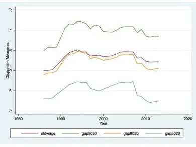
dispersion, being the early 90’s the period where a larger growth rate of the standard deviation was verified, whereas from the 00’s onwards the variation was negligible or even negative.11
In fact, most years in the beginning of that period registered a small increase contrasting with the timespan of 2006 to 2011 where only 2009 saw an increase in the standard deviation of the logarithm of real hourly wages.12Hence, this picture diverges markedly from the one observed
in Card, Heining, and Kline (2013), where these measures grow throughout the whole period. Furthermore, while in the former the higher growth rates were observed until the early 1990’s, in the latter these increased from the mid-90’s onwards.
Figure 1: Measures of Wage Dispersion
This figure includes the standard deviation of the logarithm of real hourly wages along with the gaps between the 80th and 50th percentiles, the 80th and 20th percentiles and the 50th and 20th percentiles, which are normalized since these variables consist on the differences in
percentiles divided by the corresponding gaps of a normally distributed variable.
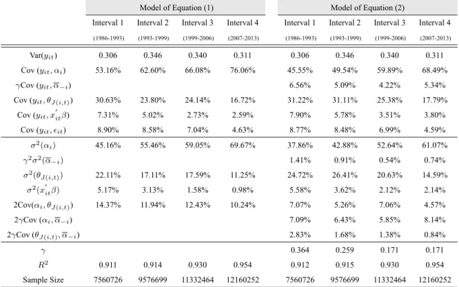
With this is mind, the estimation of equations (1) and (2) was performed and the corresponding variance decomposition is presented in Table 1.
First of all, it is possible to confirm the recent decline in wage dispersion noticed in the graphical analysis, with the variance of wages reaching a level in the last interval close to the one in the initial interval. In the case without the peer effect, it can be seen that worker time-invariant characteristics account for a large extent of the variance of wages, between 53% and 76% (in fact, it is increasing over time). Heterogeneity of firms contributes between 31% and 17% (it is 11The exceptions are the years of 1995, 1996 and 1997, with the latter registering a quite pronounced decline (the
standard deviation declined 3.30% when compared to 1996).
12The highest decline in our sample was verified in 2008: the standard deviation of the logarithm of real hourly
Model of Equation (1) Model of Equation (2)
Interval 1 Interval 2 Interval 3 Interval 4 Interval 1 Interval 2 Interval 3 Interval 4
(1986-1993) (1993-1999) (1999-2006) (2007-2013) (1986-1993) (1993-1999) (1999-2006) (2007-2013)
Var(yit) 0.306 0.346 0.340 0.311 0.306 0.346 0.340 0.311
Cov (yit, αi) 53.16% 62.60% 66.08% 76.06% 45.55% 49.54% 59.89% 68.49%
γCov (yit, α−i) 6.56% 5.09% 4.22% 5.34%
Cov (yit, θJ(i,t)) 30.63% 23.80% 24.14% 16.72% 31.22% 31.11% 25.38% 17.79%
Cov (yit, x′itβ) 7.31% 5.02% 2.73% 2.59% 7.90% 5.78% 3.51% 3.80%
Cov (yit, ϵit) 8.90% 8.58% 7.04% 4.63% 8.77% 8.48% 6.99% 4.59%
σ2(αi) 45.16% 55.46% 59.05% 69.67% 37.86% 42.88% 52.64% 61.07%
γ2σ2(α−i) 1.41% 0.91% 0.54% 0.74%
σ2(θ
J(i,t)) 22.11% 17.11% 17.59% 11.25% 24.72% 26.41% 20.63% 14.59%
σ2(x′itβ) 5.17% 3.13% 1.58% 0.98% 5.58% 3.62% 2.12% 2.14%
2Cov(αi, θJ(i,t)) 14.37% 11.94% 12.43% 10.24% 7.07% 5.26% 7.06% 4.57%
2γCov (αi, α−i) 7.09% 6.43% 5.85% 8.14%
2γCov (θJ(i,t), α−i) 2.83% 1.68% 1.38% 0.84%
γ 0.364 0.259 0.171 0.171
R2 0.911 0.914 0.930 0.954 0.912 0.915 0.930 0.954
Sample Size 7560726 9576699 11332464 12160252 7560726 9576699 11332464 12160252
Table 1: Variance Decomposition of Equations (1) and (2)
Equation (1) corresponds to the specification without the peer effect whereas equation (2) includes that effect. This table presents the two alternative variance decompositions proposed in equations (3) and (4). It also includes, in the context of the model of equation (2), the
estimated effect that the quality of peers has on a worker’s wage (γ).
decreasing over time). Taking into account the decomposition of equation (3), it is noticeable that the person effects become more variable over time while the firm effects and the covariate index (x′itβ) turn out to be less variable. Moreover, the role of the covariance between person
and firm effects has also a smaller role, ranging between 10% and 14%. Therefore, sorting of high skilled workers into high wage firms (positive assortative matching) contributes to wage dispersion. These results diverge from the ones presented by Card, Heining, and Kline (2013), which is intuitive since their case is contrary to ours as inequality is increasing in Germany.
Secondly, if the case with peers is considered, gauging the impact of the quality of peers on individual wages is possible: on average, a one standard deviation increase in the average of the person effects of a worker’s peers (peer quality) results in an increase of hourly wages by 6.57%, 5.61%, 4.28% and 4.80% in intervals 1, 2, 3 and 4, respectively.13 Looking at the variance
decomposition, the contribution of the peer effect to wage dispersion ranges between 4.2% and
13This result is obtained by multiplying gamma with the standard deviation of the peer effect which takes the
6.6%. Even though this effect was declining between 1986 and 2006, it increased again in the latest period. This observation may be twofold: there has been a decline in the number of occupations where peer pressure and knowledge spillovers are mainly present and/or the rise in qualifications people have when entering the labor market leads them no longer to acquire that much knowledge from more experienced co-workers. Analogous to the conclusion in the situation without the peer effect, person effects have the highest contribution, which is increasing over time, while firm effects are also relevant but their contribution has been declining (this may be the outcome of the rising representativeness of the minimum wage, that has been comprising more and more workers and/or of collective bargaining). One interesting conclusion is that the inclusion of the peer effect decreases the proportion of the wage variation that is explained by the person effects and slightly increases the ones of the firm effect and the covariate index.14
In addition, accounting for the variance decomposition of equation (3), the same conclusions hold for the variation of person effects and firm effects. Firstly, the increase in the variation of the person effects over time may have been caused by the entrance in the labor market of high skilled workers (with a higher person effect) concomitant with the permanence of less skilled workers, which increases the dispersion of person effects. On the other hand, the decrease in firm effects may arise due to smaller profits, which decreases the shared rents in firms that did so. Moreover, the recent crisis may have led to a reduction of labor costs through a decline in flexible wage components whose outcome would also be a decline in the variation of this variable. On the other hand, firm effects are most of the times attributed to the existence of market failures which are a source of labor market power.15 With the recent economic crisis,
less workers were available to move to another job because of the prominent need of job security observed in those times. Consequently, immobility of workers increased, leading firms that did not have or had little monopsony power to acquire it. This may have resulted in a lesser role in wage dispersion by firm effects because the existing differences of market power amongst firms were reduced.
14This goes against what was found for a region of Italy by Battisti (2013), where the contribution of the firm
effects declines significantly with the inclusion of the peer effect.
15Félix and Portugal (2016) identify the existence of search frictions (due to, for instance, imperfect information
The variation of the peer effect has a small contribution to wage dispersion (between 0.5% and 1.4%). Matching between high skilled workers and high wage firms is also relevant, even though in a smaller proportion than before (ranges between 4.6% and 7%). An additional impact is the one of high skilled individuals sorting themselves into high quality peer groups, contributing between 5.8% and 8% to wage inequality. This effect increased in the latest period, after a continuous decline. The covariance between high wage firms and high quality peers contributes between 0.8% and 2.8% to wage dispersion.
Comparing these outcomes with the ones on the full sample (see Table 4 in the appendix), person effects are still the factor contributing more to wage dispersion, but in a smaller value than in any of the periods, whilst only the first interval has a higher contribution of firm effects than the correspondent value in the full model. Hence, splitting into periods is giving more weight to person effects in detriment of firm effects. The contribution of the variation of person effects is also smaller in the full model, while firm effects have a similar weight in both cases. Positive assortative matching has a higher contribution in the full model (18%) than in any interval.16 Relatively to the inclusion of the peer effect, a one standard deviation increase in
peer quality results in a wage increase of 3.91%, on average, ceteris paribus, which is somewhat lower than what was noticed in the decomposition into periods. Battisti (2013) found this effect to be of 7.81% for Veneto, Italy and Lengermann (2002) suggests this effect takes the value of approximately 3% for the state of Illinois, United States of America. In Cornelissen, Dustmann, and Schönberg (2013), small peer effects were also found for Germany. The authors advance that this outcome likely derives from the prominent presence of occupations where workers don’t observe the performance of their peers (which leads to a low peer pressure) and/or the lack of high skilled and knowledge intensive jobs (which are the ones where knowledge spillovers are more impactful). Relatively to the contribution of person effects to wage dispersion in this case, it is only lower than the correspondent in the full model (49.21%) in the first period, whereas for firm effects it is larger in the first two periods. In the full model, the contribution of the peer effect is smaller in value than in any of the periods17. In the division into intervals, the
16As shown in Andrews et al. (2012), the estimation obtained for assortative matching in the division into intervals
may be downward biased due to less mobility of workers among firms.
17The contribution of the person effect variation is lower in the full model, with the exception of the first period;
importance of positive assortative matching is much lower than in the full model, sorting of high skilled workers into high quality peer groups has a much higher contribution to wage dispersion and the covariance between high wage firms and high skilled peers is similar in both cases, only with the latest interval presenting a smaller value.
6.1 Alternative specifications
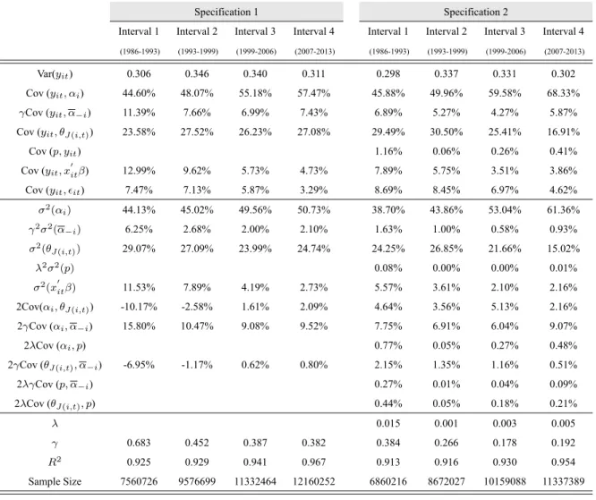
When firm effects are time-varying (have firm-year fixed effects), the contribution of person effects to the variance of wages suffers a slight decline in all intervals except in the last one which observes a larger decrease, which is observable in Table 2.
Specification 1 Specification 2
Interval 1 Interval 2 Interval 3 Interval 4 Interval 1 Interval 2 Interval 3 Interval 4
(1986-1993) (1993-1999) (1999-2006) (2007-2013) (1986-1993) (1993-1999) (1999-2006) (2007-2013)
Var(yit) 0.306 0.346 0.340 0.311 0.298 0.337 0.331 0.302
Cov (yit, αi) 44.60% 48.07% 55.18% 57.47% 45.88% 49.96% 59.58% 68.33%
γCov (yit, α−i) 11.39% 7.66% 6.99% 7.43% 6.89% 5.27% 4.27% 5.87%
Cov (yit, θJ(i,t)) 23.58% 27.52% 26.23% 27.08% 29.49% 30.50% 25.41% 16.91%
Cov (p, yit) 1.16% 0.06% 0.26% 0.41%
Cov (yit, x
′
itβ) 12.99% 9.62% 5.73% 4.73% 7.89% 5.75% 3.51% 3.86%
Cov (yit, ϵit) 7.47% 7.13% 5.87% 3.29% 8.69% 8.45% 6.97% 4.62%
σ2(αi) 44.13% 45.02% 49.56% 50.73% 38.70% 43.86% 53.04% 61.36%
γ2σ2(α
−i) 6.25% 2.68% 2.00% 2.10% 1.63% 1.00% 0.58% 0.93%
σ2(θJ(i,t)) 29.07% 27.09% 23.99% 24.74% 24.25% 26.85% 21.66% 15.02%
λ2σ2(p) 0.08% 0.00% 0.00% 0.01%
σ2(x′
itβ) 11.53% 7.89% 4.19% 2.73% 5.57% 3.61% 2.10% 2.16%
2Cov(αi, θJ(i,t)) -10.17% -2.58% 1.61% 2.09% 4.64% 3.56% 5.13% 2.16%
2γCov (αi, α−i) 15.80% 10.47% 9.08% 9.52% 7.75% 6.91% 6.04% 9.07%
2λCov (αi, p) 0.77% 0.05% 0.27% 0.48%
2γCov (θJ(i,t), α−i) -6.95% -1.17% 0.62% 0.80% 2.15% 1.35% 1.16% 0.51%
2λγCov (p, α−i) 0.27% 0.01% 0.04% 0.09%
2λCov (θJ(i,t), p) 0.44% 0.05% 0.18% 0.21%
λ 0.015 0.001 0.003 0.005
γ 0.683 0.452 0.387 0.382 0.384 0.266 0.178 0.192
R2 0.925 0.929 0.941 0.967 0.913 0.916 0.930 0.954
Sample Size 7560726 9576699 11332464 12160252 6860216 8672027 10159088 11337389
Table 2: Alternative specifications of Equation (2)
Specification 1 corresponds to equation (2) but including time-varying firm effects whereas specification 2 corresponds to equation (3), which differs from equation (2) due to the inclusion of a measure of productivity.
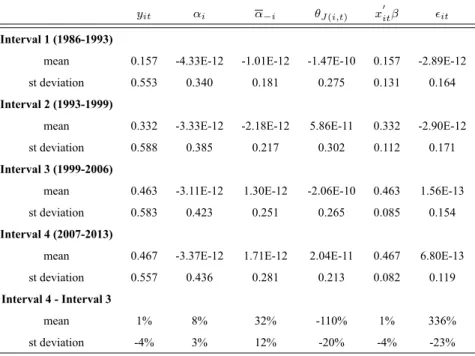
latest intervals). The contribution of the covariate index is larger in all periods, as is the peer effect. The effect that a one standard deviation increase in the quality of the co-workers has on wages is an increase of 13.84%, 9.63%, 8.25% and 8.09%, respectively, being much larger than in the original case. This seems to struck a discordant note when compared with the opposite finding in (Lengermann 2002). Actually, this result implies that firms that choose to increase the quality of workforce are, at the same time, decreasing the wage premium paid to their workers. A possible explanation for this is the increase in the supply of high skilled workers associated with a decrease in wages (when is not matched by a demand increase), effect that is further enhanced in the latest period due to a decline in labor demand caused by the economic crisis. In fact, if we look at the mean of the peer effect (which measures the average quality of the workforce), from the third to the fourth period there has been an increase of approximately 32% of the mean value of this variable (refer to Table 3 in the appendix). Concerning the contribution of the variation of each component, person effects are less variable, as well as firm effects. In this setting, the contribution of the variation of the peer effect is larger than in the original setting (ranging between 2% and 6%), in the first two periods negative assortative matching is observed and the contribution of the covariance between the quality of the peer group and firm heterogeneity is also negative. A major difference in this case is the large contribution of sorting of workers into high skilled peer groups (ranging between 9.1% and 15.8%). Contrasting these conclusions with the full model (Table 4 in the appendix), person effects have a lower contribution, as does the peer effect. In the full model, the contribution of the firm effect goes to zero. Therefore, in this specification for the full model, the contribution of firm effects is “given” to the other two effects, which is not as observable in the division into time intervals18. The full model entails negative
assortative matching, much higher than in any interval, contrasting with the large contribution of sorting of high skilled workers into high quality peers which is much larger than in any period. A more relevant outcome is the increase of wages by 13.21% due to an increase of a one standard deviation in the peer effect.
In including a measure of productivity, by estimating equation (6), an increase of a standard 18In the case of the contribution of the variation of person, peer and firm effects: they are much higher in the
deviation in the peer effect impacts wages slightly more than in the original case (6.97%, 5.82%, 4.38% and 5.30%, respectively). Considering the variance decompositions analysed, the results are identical to the original model with the difference that the positive assortative matching is lower. The contribution of productivity, its variation and the covariance between it and person effects, peer effect and firm effects are rather muted. When comparing this formulation to the full model specification, the same deductions of the comparison made in the context of equation (2) hold. These conclusions likely result from the fact that the firm effect already absorbs any impact productivity would have on wages.
7 Conclusion
The main purpose of this study was to investigate whether the quality of the group of co-workers of an individual had an impact in the dispersion of inequality, observing how this contribution would vary over time, along with other more common sources of variation like person and firm characteristics. Additionally, it set out to verify if alternative specifications such as enabling firm effects to vary over time and including productivity would change any of the aforementioned effects. As found in previous empirical research, peer spillovers have a small, but relevant, positive effect on the logarithm of real hourly wages. In this case, the contribution it has for wage dispersion ranges from 4.3% to 6.6%, being slightly lower (approximately 4%) for the full model. Nevertheless, if firm-year fixed effects are introduced, the values obtained are much higher.
peer groups (the covariance between the person and peer effects contributes between 5.9% and 8% to wage dispersion). The mentioned effects do not suffer alterations when accounting for different firm productivity levels, which likely results from the retention by the firm effect of any impact this variable might have. However, when considering time-varying firm fixed effects, the variation of person and firm effects present a more reduced contribution to the variance of wages, being the contribution of the variation of the peer effect larger than in the original setting.
On balance, this thesis can be added to the recent literature on peer effects in the workplace, particularly to their impact on wages and its dispersion. It contributes to the study of wage dispersion in Portugal by complementing the existing knowledge of the period until the mid-1990’s and extending it for more recent years.
8 Bibliography
Abowd, John M., Francis Kramarz, and David N. Margolis. 1999. “High Wage Workers and High Wage Firms.” Econometrica67 (2): 251–333.
Andrews, M. J., L. Gill, T. Schank, and R. Upward. 2012. “High Wage Workers Match with High Wage Firms: Clear Evidence of the Effects of Limited Mobility Bias.” Economics Letters
117: 824–27.
Angrist, Joshua D. 2014. “The Perils of Peer Effects.” Labour Economics30: 98–108.
Arcidiacono, Peter, Gigi Foster, Natalie Goodpaster, and Josh Kinsler. 2012. “Estimating Spillovers Using Panel Data, with an Application to the Classroom.” Quantitative Economics
3: 421–70.
Battisti, Michele. 2013. “High Wage Workers and High Wage Peers.” Ifo Working Paper. Vol. 168.
Bloom, Nicholas, James Liang, John Roberts, and Zhichun Jenny Ying. 2015. “Does Working from Home Work? Evidence from a Chinese Experiment.” Quarterly Journal of Economics
130 (1): 165–218.
Card, David, Ana Rute Cardoso, and Patrick Kline. 2016. “Bargaining, Sorting, and the Gender Wage Gap: Quantifying the Impact of Firms on the Relative Pay of Womem.” Quarterly Journal of Economics131 (2): 633–86.
Card, David, Patrick Kline, Jörg Heining, and Patrick Kline. 2016. “Firms and Labor Market Inequality: Evidence and Some Theory.” IZA Discussion Paper9850.
Cardoso, Ana Rute. 1997. “Workers or Employers: Who Is Shaping Wage Inequality?” Oxford Bulletin of Economics and Statistics59 (4): 523–44.
———. 1998. “Earnings Inequality in Portugal: High and Rising?” Review of Income and Wealth44 (3): 325–43.
———. 1999. “Firms’ Wage Policies and the Rise in Labor Market Inequality: The Case of Portugal.” Industrial & Labor Relations Review53 (1): 87–102.
———. 2004. “Wage Mobility: Do Institutions Make a Difference? A Replication Study Comparing Portugal and the UK.”IZA Discussion Paper1086.
Cardoso, Ana Rute, Paulo Guimarães, and Pedro Portugal. 2012. “Everything You Always Wanted to Know about Sex Discrimination.” IZA Discussion Paper, no. 7109.
Cornelissen, Thomas, Christian Dustmann, and Uta Schönberg. 2013. “Peer Effects in the Workplace.” IZA Discussion Paper, no. 7617.
Davis, Steve J, and John Haltiwanger. 1991. “Wage Dispersion between and within U.S. Man-ufacturing Plants, 1963-86.” Brookings Papers on Economic Activity1991 (1991): 115–200. Dickens, William T, Lorenz Goette, Erica L Groshen, Steinar Holden, Julian Messina, Mark E Schweitzer, Jarkko Turunen, and Melanie E Ward. 2007. “How Wages Change: Micro Evidence from the International Wage Flexibility Project.” Journal of Economic Perspectives21 (2): 195– 214.
Dunne, Timothy, Lucia Foster, John Haltiwanger, and Kenneth Troske. 2000. “Wage and Pro-ductivity Dispersion in U.S. Manufacturing: The Role of Computer Investment.” NBER Work-ing Paper7465.
Faggio, Giulia, Kjell Salvanes, and John Van Reenen. 2007. “The Evolution of Inequality in Productivity and Wages: Panel Data Evidence.” NBER Working Paper13351.
Félix, Sónia, and Pedro Portugal. 2016. “Labor Market Imperfections and the Firm’s Wage Setting Policy.” IZA Discussion Paper10241.
Groshen, Erica L. 1991. “Sources of Intra-Industry Wage Dispersion: How Much Do Employers Matter?” Quarterly Journal of Economics106 (3): 869–84.
Guimarães, Paulo, and Pedro Portugal. 2010. “A Simple Feasible Procedure to Fit Models with High-Dimensional Fixed Effects.” Stata Journal10 (4): 628–49.
Kremer, Michael. 1993. “The O-Ring Theory of Economic Development.” Quarterly Journal of Economics108 (3): 551–75.
Lindquist, Matthew J, Jan Sauermann, and Yves Zenou. 2015. “Network Effects on Worker Productivity.” CEPR Discussion Paper10928.
Machado, José A. F., and José Mata. 2001. “Earning Functions in Portugal 1982-1994: Evi-dence from Quantile Regressions.” Empirical Economics26: 115–34.
Martins, Pedro S., and Jim Y. Jin. 2010. “Firm-Level Social Returns to Education.” Journal of Population Economics23 (2): 539–58.
Mas, Alexandre, and Enrico Moretti. 2009. “Peers at Work.” American Economic Review99 (1): 112–45.
Pereira, Pedro T., and Pedro S. Martins. 2000. “Does Education Reduce Wage Inequality? Quantile Regressions Evidence from Fifteen European Countries.” IZA Discussion Paper, no. 120.
Sacerdote, Bruce. 2001. “Peer Effects with Random Assignment: Results for Dartmouth Room-mates.” The Quarterly Journal of Economics116 (2): 681–704.
Van Reenen, John. 1996. “The Creation and Capture of Rents: Wages and Innovation in a Panel of U.K. Companies.” Quarterly Journal of Economics111 (1): 195–226.
Appendix
yit αi α−i θJ(i,t) x
′
itβ ϵit
Interval 1 (1986-1993)
mean 0.157 -4.33E-12 -1.01E-12 -1.47E-10 0.157 -2.89E-12
st deviation 0.553 0.340 0.181 0.275 0.131 0.164
Interval 2 (1993-1999)
mean 0.332 -3.33E-12 -2.18E-12 5.86E-11 0.332 -2.90E-12
st deviation 0.588 0.385 0.217 0.302 0.112 0.171
Interval 3 (1999-2006)
mean 0.463 -3.11E-12 1.30E-12 -2.06E-10 0.463 1.56E-13
st deviation 0.583 0.423 0.251 0.265 0.085 0.154
Interval 4 (2007-2013)
mean 0.467 -3.37E-12 1.71E-12 2.04E-11 0.467 6.80E-13
st deviation 0.557 0.436 0.281 0.213 0.082 0.119
Interval 4 - Interval 3
mean 1% 8% 32% -110% 1% 336%
st deviation -4% 3% 12% -20% -4% -23%
Table 3: Descriptive Statistics
Full Model
(1) (2) (3) (4)
Var(yit) 0.340 0.340 0.340 0.331
Cov (yit, αi) 51.08% 49.21% 62.72% 49.13%
γCov (yit, α−i) 3.75% 13.11% 3.91%
Cov (yit, θJ(i,t)) 27.49% 25.42% 0.89% 24.16%
Cov (p, yit) 1.09%
Cov (yit, x′itβ) 9.38% 10.15% 12.24% 10.22%
Cov (yit, ϵit) 12.04% 11.48% 11.19% 11.50%
σ(αi) 41.02% 39.09% 64.21% 39.29%
σ(α−i) 0.45% 5.13% 0.50%
σ(θJ(i,t)) 17.61% 16.42% 9.08% 15.64%
σ(p) 0.07%
σ(x′itβ) 7.63% 8.10% 17.37% 8.02%
Cov(αi, θJ(i,t)) 18.20% 14.06% -11.49% 12.40%
Cov (αi, α−i) 3.92% 20.56% 4.11%
Cov (αi, p) 0.89%
Cov (θJ(i,t), α−i) 2.38% -5.50% 2.27%
Cov (p, α−i) 0.15%
Cov (θJ(i,t), p) 0.78%
λ 0.013
γ 0.217 0.479 0.228
R2 0.885 0.885 0.887 0.885
Sample Size 37873532 37873532 37873532 34534575
Table 4: Variance Decomposition in the Full Model