UNIVERSIDADE TÉCNICA DE LISBOA
INSTITUTO SUPERIOR DE ECONOMIA E GESTÃO
MESTRADO EM ECONOMIA
Non-constant Time Discounting and Asset Pricing
Miguel Atanásio Lopes Carvalho
Orientação: Doutor Paulo Meneses Brasil de Brito
Júri:
Presidente : Doutor Paulo Meneses Brasil de Brito
Vogais : Doutor João Manuel Gonçalves Amaro de Matos e
Doutor António Manuel Gonçalves da Silva Saragga Seabra
Julho 2005
Glossary
• discount factor : d.f. = —e where F{t) is the discount function. For f[t) = Q1 \ve have d.f. = ,6
• discount function : function F{T,t) that stands for the subjective weight given to the instant Utilities of different periods, when aggregating for the total in- tertemporal utility. It is a function of r the time of evaluation and t the time gap between the time of the evaluation and the time of the instantaneous utility considered.
• discount rate : d.r. = where F{t) is the discount function. For F{t) = (d1
we have d.r. = —Inp
• exponential discount : the most common time discount also called geometric discount (because of the geometric series p1) or constant discount (because of
the constant discount factor and rate). It is represented by F{t) = p1 with
discount factor p or by F{t) = e~pt with discount rate p. Exponential discount
is equivalent to stationary and consistent discount.
• hyperbolic discount : subjective stationary time discount whose discount func- tion is a generalized hyperbola. The most common form is given by F{t) = (1 + at)~b,a whose discount rate is where o > 0 and close to 1 and 6 > 0
usually close but lower than 1. The discount rate starts as b and tends to zero.
• present-biased preferences : any time discount where the immediate discount rate is higher than the médium and long rim discount rates, (non-stantard definition)
• quasi-hyperbolic discount : subjective discrete time discount, which resembles 2
in some way the hyperbolic discount. Its discount function is given by F(0) = 1 and F{n) = I36n.
• stationary preferences : at difFerent periods future events are discounted in the same fashion, that is F is just a function of t and not of r.
• time inconsistency : behaviours/preferences are said to be time inconsistent if (in the absence of any new information) agents at some period have new optimal plans and want to discard former ones. Formally there is time inconsistency 7^ F(r+A,'í2-A) ^or some A, that is the discount factor between
Abstract
We analyze in a simple three period model, how the time inconsistency of agents affects the endogenous rates of return of assets determined by the equilibrium in an exchange econ- omy with consumption and exogenous endowments. We model the intertemporal decisions according to Phelps and Pollak (1968) - taking the actions of the agents as the rcsult of a game between different "selves" in different decision nodes - and consider the most common case of "present-biased" preferences. The rates will be formally different from the consistency case. namely they will depend on future endowments, both with stochastic and deterministic endowment processes. This enables the distinction between time consistent and inconsistent preferences from the data. It also implies that the estimation of expected endowments from market data depends on the type of preferences of the representative agent. Under endow- ment uncertainty we conclude that even though the determination of the rates of return can be largely affected this does not lead to significantly different risk premia. Moreover distinctive mformation gaps between "selves" does not account for distinctive results, even though the results depend strongly on their interaction. Finally, we propose and apply to the different cases, a new method for discount comparison.
Keywords ; Intertemporal Choice, Intertemporal Consumer Choice, Noncooperative Games, Microeconomic Behaviour: Underlying Principies, Exchange and Produc- tion Economies, Asset Pricing.
Contents
1 Introduction 7
2 Non-constant Time Discounting and Literature Review 12
2.1 Time Inconsistency 12
2.2 Earlier Literature on Non-constant Discount 14
2.3 Recent Studies 19
2.4 Criticai Analysis of Time Inconsistency 25
2.5 Related Asset Pricing Literature 27
3 General Equilibrium Asset Pricing 28
3.1 Naive agents 29
3.2 Sophisticated agents 33
3.2.1 Sophisticate!s Backward Induction 33
3.2.2 Analysis 37
4 Time inconsistency Facing a Risky and a Riskless Asset 42
4.2 Tlmv poriods 45
4.3 Analysis 43
4.3.1 Bond retu rn with uncertainty 49
4.3.2 Risk Premium under Hyperbolic Discounting 50
5 Conclusions 55
6 References 57
E p'rá amanhã Bem podias fazer hoje
Porque amanhã sei que voltas a adiar (...)
E p'rá amanhã
Bem podias viver hoje
Porque amanhã quem sabe se vais cá estar (...)
E p'rá amanhã
Deixa lá não faças hoje
Porque amanhã tudo se há-de arranjar1
António Variações
1 Introduction
Macroeconomical models concerning intertemporal decision making usually as- sume time consistent preferences. That is to say that agents" optimal choices are independent of the time of evaluation (in the case of perfect foresight obviously). In a deterministic setting an individual will always take the decisions he planned to take some time ago.
Models also assume additive preferences2 which means that instantaneous Utili-
ties are aggregated acioss time periods and across states of nature using a sum. It is straightforward to see that (time stationary^) additive preferences are time con- sistent if and only if there is no time discount at ali or if the discount is constant. If 'Ifs for tomorrow! / You could well do it today / Because I know you ll postpone it again tomorrow It s for tomorrow! / You could well live today / Because who knows if you ll he here tomorrow // ffs for tomorrow! Let it be, don't do it today / Because tomorrow you'll manage everything
2More on different aggregate utiiity structures in Backus, Routledge and Zin (2004)
3Time stationarity means that instantaneous Utilities are discounted with the same discount function regardless of
the decision period. In other words the discount weight depends solely on the time gap f between the decision and the enjoyment. In this study only stationary preferences are considered because non-stationaritv at the macroeconomical levei seems unreasonable. For an approach with non-stationary preferences see Kocherlakota (2001),
the discouiit factor is to be constant the discount function is an exponential. That is whv constant discount is sometimes referred as "exponential" discount.
The present work is intended to explore the consequences of relaxing this hypoth- esis considering non-constant discount rates. We sum up the work that has heen done and present a basic general equilibriurn asset pricing model.
As a matter of fact there has been growing evidence that agents do not have time consistent preferences. Borrowing an example from Ainslie (1991), "a majority of adults report that they uiould rather have $50 immediately than $100 in 2 years, but alrnost no one prefers $50 in 4 years over $100 in 6 years, even though this is the same choice seen at 4 years greater distance". The discount factor between today and two years from today (a two year gap) is bigger than between four and six years of distance (two year gap also), technically speaking the discount rate is not constant. Constant (or exponential) discount means having the same levei of impatience between today and a month from now, and between the Ist of January and the Ist of February of 2100. No experiment may ever support this assump- tion. Experimental evidence indicates that time is not discounted with exponen- tial discount functions (and constant discount rates) but generalized hyperbolic-like discount functions (with decreasing discount rates). Individuais are said to have present-biased" preferences because small time gaps in the near future and long time gaps in the far future are perceived equally.
This raises a time consistency problem. Using Ainslie's example, an individual who opted for the $100 in 6 years will probably change his mind after 4 years. He will prefer having $50 by then. How agents act given this inconsistency and how
their behaviour should he modelled is however an open question.
Two basic theoretical hypothesis have been considered. Agents may not realize their inconsistency and exhibit the so-called ''naive" behaviour. They naively believe they will pursue previous optimal plans but keep engaging in new ones. Typically naive agents continuously overconsume today relying on their future savings abili- ties. Everyday evidence is easy to find. On the other hand agents realizing their time inconsistent preferences may a have rational attitude and try to follow a time consistent plan. Taking in mind that their future impulses cannot be controlled but can be foreseen, the so-called "sophisticated1" individuais are able to depict a plan
that will actually be followed. When someone chooses to fulfill some duty today in- stead of postponing it, just because he knows he would postpone it again tomorrow. that person is acting like a sophisticate. This behaviour is modelled considering a subgame perfect equilibrium of a game between the "selves" of different periods.
Statements like "do not let me do this or that" is also an everyday example of a sophisticated attitude but of a different kind. The individual knows he will be wanting to do something non-optimal from today's perspective and wishes to bind his future actions, that is he wants to precommit his future actions. Sophisticates would like to have some commitment devices (illiquid assets is a financial example) and so different models are classified according to the existence and tvpe of these devices. Sophisticates come in three Havours: no-commitment, partial-commitment and full-commitment.
Our focus will be on asset pricing and our motivation on exploring the impli- cations of inconsistency on the trade-off between risk and return of assets on the
individual and on the general equilibrium levei. Thus we will he able to address both behaviour and inacroeconomic changes. And wc emphasize the later one, because the time inconsistency literature deals mainly with partial equilibrium results.
Likewise there is few work on non-constant discount with uncertainty. The risk aversion is strongly related with the attitude of agents towards time so some changes would be expected. In this sense we shall examine the equity risk premia for it is widely known that the estimated risk aversion leveis do not account for the observed high premia.
We present an application of these ideas in a simple general equilibrium three period asset pricing model in a pure exchange economy. Three periods is the min- imum number with which inconsistency issues arise; in a two period model, the last period problem is always straightforward. The differences between naives and sophisticates are clarified. Deterministic and stochastic endowment processes are both analyzed. When comparing the exponential and the hyperbolic discounts we refrain from pointing out quantitative differences that simply disappear in a calibra- tion. Observationally distinguishable qualitativo differences will be our main point. Second we introduce a compensated parameter variation so that calibration-proof quantitative conclusions are possible.
We show that the intertemporal trade-off of sophiscates is more complex than that of naives or time consistent individuais. It is not just a savings/consumption choice but also a confhct between today's and tomorrow's optimal plans. On one hand present-bias puts a strong emphasis on immediate consumption relying on future savings. On the other knowing that tomorrow the agent will have the same
attitude, he will have an incentive to save more today. As a consequence of this complex equilibrium, short-run interest rates at time t will not only depend on the endowments of time t and t + 1 but on future (expected) endowments. This is true in the absence of long-nm assets, as it happens in our model. Moreover the elasticity of sub-titution levei is a fundamental parameter for the outcome of the trade-off. High elasticity (utility function with positive homogeneity degreej may lead to an intriguing increase in savings in case of a future endowment growth. A natural consequence of these conclusions is that time consistent and inconsistent preferences are observationally unlike concerning general equilibrium asset prices. This contradicts the results of Kocherlakota (2001).
It is shown in the last section that stochastic endowment and asset pavoffs pro- cesses do not introduce any new feature comparing with the deterministic situation. The strategical interaction between selves remains broadly unchanged including for different information structures. In the end we focus on the equity premium puz- zle and conclude that inconsistent preferences should not account for significantly different risk premia.
The present work is structured as following: section 2 contains a review on time inconsistent discounting, in section 3 we solve simple asset pricing models without uncertainty and discuss different issues mentioned in section 2. section 4 contains the main model with a riskless and a risky asset where we analyze the consequences on risk premia, and our conclusions are summarized in section õ.
2 Non-constant Time Discounting and Literature Review
Xext \ve suni up important facts on time discount and present a survey (followed h\' a criticai analysis) on non-constant time discount. Some of the few work on asset pricing is also presented.
2.1 Time Incousistency
Time discount is used when agents have additive Utilities (we will not consider other cases) and perceive equal instantaneous utility leveis differently depending on the time gap between today and the enjoyment. It enables the matching between two intertemporal plans through the attribution of different time weights when ag- gregating instantaneous Utilities.
In a deterministic and perfect information economy can be easily shown (see Strotz (1956)) that the only possibility of having dynamically consistent decisions, that is tomorrow's optimal choice from today's perspective being exactly the same as tomorrow"s optimal choice from tomorrowT perspective, is considering exponential discounting, that is a constant discount rate. Note that with F{t) — /T being the discount function we have
F{p) _ F{q) _ nA y A Fip + A) F{q + A) ' P'9'
meaning that when we compare two events with utility leveis assigned to different periods, only the time interval A between them and not the time between today (f = 0) and either of them {p or q), does matter. Tliis implies that whenever the agent matches the present value of the utility of both, he will take the same
choice. Reasoning graphically Ainslie (1992) points out that "discountmg curves must cross to produce ambivalence". Discounting curves represent present values of future events depending on the time of evaluation. When they cross we have inconsistency. Just before the "crossing time" there is one action that is preferred towards the other. But just after the crossing time, the agent would take exactly the opposite decision.
There is quite a lot of everyday evidence that we do not have time consistent preferences that is agents do not discount the time at a constant rate. Statements or "self-promises" like "77/ eat just this ice cream, and start my diet tomorrouj" and "7 have postponed this work for too long, I must start it tomorrow" are com- mon examples. Other more complex economic examples will be mentioned below. We underline that this kind of behaviour of changing our own plans and of self- enforcement, is not due to uncertainty or new information available that obviouslv would lead to a change in plans, but entirely to time inconsistency. We often post- pone unpleasurable actions and advance pleasurable ones relatively to our previous plans.
This preferences anomaly (sometimes referred as present-bias), if we take the exponential discount as benchmark, is the most commonly considered in the time inconsistency literature, which mathematically speaking stands for a decreasing dis- count rate in the immediate future. But there is another anomaly regarding the long-run. As we move faraway from the present the dates become almost irrelevant. so that the utility of a revenue (or cost) in 2060 or 2061 perceived todav is almost the same. Mathematically the discount rate tends to zero. As we will be dealing with 3 period models this detail will not come up. Its mathematical complexity is
prohably the reason for which it was despised in the literature.
2.2 Earlier Literature on Non-constaut Discount
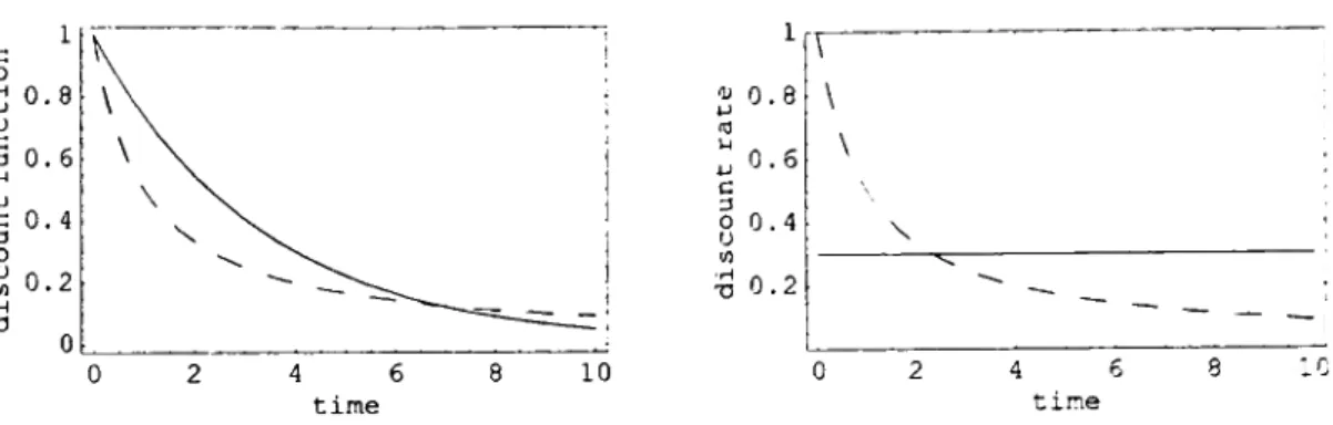
Though not explicit, Bòhm-Bawerk's work "'Positive Theorie des Kapitals" (1889) is the first reference on non-constant discount Pointing out that "there may be a strong difference between an enjoyment which offers itself at the very instant, and one which does not; while, on the other hand, there may he a very small difference, or no difference at ali, between an enjoyment which is pretty far away, and one which is farther away". That is the immediate discount is high and the faraway future discount in nearly zero. Obviously he could not realize the consequences, for there was not any discount notion, and it was not until Strotz (1956) that the problem was analyzed. Strotz's work is quite revolutionary, established new concepts and is still a benchmark. Strotz suggests different behaviours due to the existence of non-constant discount rates. Based on everyday situations, he assumes (correctly) that agents discount time at a decreasing discount rate, meaning that the subjective relative weight given to two events one week apart from each other, decreases, or tends even to zero as they are further away from the present. Put simply, the discount between today and tomorrow is more or less the same as, imagine, between January 2050 and January 2055. This is depicted in Figure 1. Actually Strotz did not propose any specific discount function, but showed his ideas graphically.
Strotz speculates about the consequences of the re-evaluation of some former optimal plan, that had been pursued so far, without any new information. He argues that usually the uoptimal plan as seen today" will not be optimal as seen
0.8 0.6 0. 4 0.2
^0.8
Figure 1: Exponential e 0'3í (straight) and hyperbolic (l+í) 1 (dashed) time discount; a) discount
functions; b)discount rates
tomorrow Ubecause the discount function has been shifted 4. Strotz adds that "it
would be a mistake to conclude that, even under condítions of certainty, the optimal curve is the one which the individual will actually follow In this case he would set a new consumption curve and some time later would again recognize that he is not following the optimal curve, etc... Strotz calls this the "intertemporal tussle". Intuitively, having planned a week ago that I would lunch today at a cheap cafeteria because I should save the money for next month"s holidays to which I assigned a greater utility than the lunch, today I assign a greater utility to going to an expensive restaurant than to the savings. The main point here is that having a constant discount rate, the relative weight of the lunch and the holidays would be constant only depending on the time distance between them and not between any of them and the decision point. But if we consider the discount function that Strotz proposes, this weight also depends on the distance to the decision point0. According
'He also recognized that the only discount function that does not lead to this inconsistency, is the exponential. which he calls the "harmony" case.
5Another example reinterpreted from Strotz: some "buy it now, pay it next year" promotions clearly take
advantage of this inconsistency. Even if the instant disutility of the cost is greater than the instam utility of the purchase, postponing it can change the relation of the present-valued Utilities.
15 I
to Strotz it the agent does not recognize this inconsistency in advance, he keeps "n pudtafnig ' his "past plnns" describing a "spendthnft" trajectory.
Strotz proposes two possibilities for the agent who recognizes this tussle. He may precoinmit his future actions, that is to bind his future actions according to his present optimal plan. Statements like "do not let me do that" or self-promises are some examples of precommitment. But regarding the whole consumption plan, this means that there should be a precise time in the past where today's actions where determined and that even though the agent recognizes today their non-optimality, he will not change his acts.
The second possibility is following a "consistent planning" strategy, that accord- ing to Strotz should be "the best plan among those he will actually follow" tak- ing into account "an insight into his future unreliability". According to Strotz's point of view this implies the recognition that he is only able to set and pur- sue the optimal consumption plan for a very sraall interval of time At. So he draws his optimal consumption plan during this interval assuming that the plan is fixed after the interval. In Strotz's stock consumption model this implies having F{t - t)/F{t — t) — -iic{t)/uc{t), where r is the present time and uc is the marginal
utility of consumption. Letting t ^ t Strotz concludes erroneously (as shown below) that we will have F(0)/F(0) = —iic{t)/uc{t) at ali points, that is along ali consump-
tion periods. Ali discounting curves would then be equivalent to an exponential e^pt
with p = —F(0)/F(0).
As Pollak (1968) points out this result is intuitively wrong. It would mean that two different discounting curves would lead to the same behaviour. To see that it is
also mathernatically wrong (and following Pollak) imagine having discrete decision points distancing Aí from each other. The consumption path in the decisions points (that split the intervals) will usually not be continuous much less differentiable. It is then a mistake to admit that the differential equation is valid at ali points as Aí -> 0.
Besides being mathernatically wrong it is hard to say that Strotz"s agent recog- nizes his inconsistency. It represents a continuous recognition of the non-optimality of yesterday's plan and the setting of a new one. In other words Strotz"s agent is exactly the opposite: someone who never recognizes the inconsistency and keeps reevaluating.
Phelps and Pollak (1968) proposed a consistent model that is still used today. Working in a discrete6 Ramsey-like growth model describe the behaviour of a rep-
resentativo agent who is aware that he cannot set the actions of future generations because they will later default. They propose a game theory approach. where today"s generation plays with tomorrow's. Using backward induction. that is taking into ac- count the behaviour of tomorrow's generations (the way they will later default), the representative agent chooses his optimal consumption for his period maximizing his aggregate utility. Assuming that the future generations will have a certain constant savings rate and using the same discount function for ali generation, they find the best response (in terms of the savings rate) for that future savings rate strategy. There is a subgame perfect Nash equilibrium when the best response rate equals the future rate, and this should represent the generation"s behaviour. They call it "the second-best optimurri" in opposition to the "first best" where the representative
agent ocnild control future (lecisions, that is he would be able to precommit. In the secoud-best case the saviugs rate is clearly lower. They show that ali generations would beneht with a raise in the saviugs rate, that is this equilibrium is definitely non Pareto optimal.
The discreto discount function they use, later nicknamed as "quasi-hyperbolic" by Laibson (1996), is given by the sequence
1, 135, f362, /3ò3,...
where 3 ~ 2/3 and S ~ 0.95 according to Laibson, has two big advantages: it captures the overvaluation of the present relatively to the irnmediate future that generates the inconsistency and the game between generations, and it is mathemat- ically easily treatable. Unfortunately it fails to capture the assymptotic approach to zero of the discount rate in the far future. Note that after the second period, this function corresponds to an exponential discount, whose discount rate is constant. Figure 2 shows three possible discrete discount functions7.
H H H H H U xxxxxííHHtíXxxxxxxxxxxx 0 5 10 15 20
Figure 2: Discrete discount functions a) discount functions; h) discount rates; X - exponential e~o u: H - hyperbolic (1 + 0.3<) '; dots - <|uasi-fiyperbolic p -- í) = 0.95;
' We define the discrete discount rate as - ' ''/y1,/ / ''d
0. 8 0. 6 ( 0. 4 | 0.2 [ 0 H X X X H • • H H * ^ y • • nu.. A v HHh^^hhh' 0.5 0.4 0. 3 0.2 0. 1 10 15 20 IX
In a note appcmled to this article Pollak (1968) applies the generation conflict to a conflict inside one's mind. He calls "naive" to individuais who do not recognize their inconsistency and keep rethinking their optimal plan. This is Strotz s '"intertemporal tussle". They are naive in the sense that they believe they will follow the freshly conceived plan. In opposition he calls "sophisticated" to individuais who rnake a "consistent planning" out of their time inconsistent preferences, solving for the subgame perfect Nash equilibrium of the game between the present and the future preferences.
Being this an infinite game, the existence of a unique equilibria is a delicate issue. The authors postulate the future constancy of savings rates which in its simple framework leads to one solution. Peleg and \aagi (1973) define a Strotz- Pollak equilibrium where player p chooses the best response to the best responses of players q > p8. Goldman (1980) shows that a Strotz-Pollak equilibrium exist under
quite general conditions.
2.3 Recent Studies
Ainslie (1991) summarizes some psychology studies involving time decisions, an- alyzing their possible consequences on economic models. He starts by pointing out the example mentioned in the introduction, which is clearly a case of time inconsis- tent preferences. He also refers studies where individuais "choose annual discount rates in the thousands of percenV. Prelec and Loewenstein (1997) cite studies where the discount rate is even negative! Given this background it is hard to design a solid intertemporal decision theory.
Nevertheless Ainslie refers the hyperbolic-like discount function {b + at)~l as the
one that fits best the data. The parameters a and b should be close to one. Ainslie's motivation is to conciliate these findings with a rational behaviour. He argues that an individual when confronted with a decision between A and B (like "stay up" and "go to bed"), uses a hyperbolic discount to match the possibilities, whose result rnay be "irrational" (staying awake, because the weight given to immediate pleasure is higher than tomorrow's fatigue). But if the decision happens to be between sequences of A's and B's, he may aggregate the separate Utilities and conclude that the other option (going to bed) may be better. In this case although he prefers staying up in the immediate run, he knows he will prefer it again next time. So in order to maximize present aggregate utility he will opt for the bed.
Ainslie (1992) contains an immense number of references of psychological studies involving time decisions by individuais. He shows that there are innumerous types of behaviour and motivations observable, like commitment strategies, games inside one's mind, etc... On one hand the hypothesis proposed by other authors seem to be real, on the other it is hard to say what kind of theoretical model should be used due to the absence of a pattern9. Unfortunately the experimental studies did not
change much the way economists analyzed and modelled time inconsistency.
Laibson (1996) backed by Ainslie's work reintroduces the Phelps and Pollak (1968) model (and discount10), modelling the behaviour of a time inconsistent indi-
vidual as a conflict inside his mind, or as Laibson puts it, between different "selves". In his finite game the individual chooses a consumption/savings strategy (there is
9Prelec and Loewenstein (1997) cite innumerous and seemingly contradictory behaviours.
10Laibson argues that quasi-hyperbolic discounting "mimics the qualitative property of the hyperbolic discount
function". As we mention above, this is a very strong assumption.
an asset with exogenous return). Laibson shows that there is a unique equilibrium which is a Markov perfect equilibrium, that is one where the strategy is a function solely of the state variable, in this case the asset holdings11. In the infinite game
he considers the limit of this equilibrium. The strategy is linear in wealth, so that it is equivalent to the exponential case. Laibson remarks that observationally the two discounts are in this sense equal. However if we let the exogenous rate of return change, the elasticity of intertemporal substitution will be lower (under general con- ditions) than the inverse of the coefficient of relative risk aversion (which is constant by assumption of the utility function) as observationally, but not theoretically. hap- pens. Another very important result is that the savings rate is Pareto dominated by the savings rate that the individual would choose if we could set ali periods rates. Laibson suggests innumerous policies that would enable the consumers in some way to follow their desired consumption path given their apparent incapacity to do it by their selves.
In his next work Laibson (1997) gives the sophisticated consumer the choice between a liquid and an illiquid asset with the same rate of return. He models illiquidity assuming that the asset is sold one period after the selling decision. In the equilibrium the individual always holds some quantity of the illiquid asset, which is used to limit the future "selves" decisions. In general equilibrium (with production) this economy happens to have a high comovement of consume and income even for wealthy consumers as expected from econometric studies.
List of Possible Intertemporal Behaviours
Constant Discount Optimal plans are always consistent one with the other
Naive Believe they will be able to stick to the present opti- mal plan but keep discarding it and rethinking a new one every period
Sophisticated Recognize their inconsistent preferences and follow a subgame perfect equilibrium
no commitment Present self has no control on future selves
full-commitment Has total control on his future actions so that he fol- lows the optimal plan conceived at the initial period partial-commitment Some control on the future using real (illiquid assets that compel future savings) or mental (self-control that enables some plan to be taken for some interval of time) commitment devices
The first model in continuous time12 appears in Barro (1997) and Barro (1999),
which is basically the Ramsey (1928) model with time inconsistent preferences, more precisely with hyperbolic discounting and sophisticated agents. Assuming a strategy linear in wealth the representative agent maximizes aggregate utility taking into account that the continuum of "selves" that follow will use the same strategy. As Laibson (1996) already pointed out, Barro shows that in the case of logarithmical utility the substitution and income effects cancel out and the model is equivalent to the Ramsey model with exponential discount, just having a lower savings rate. Once again they are observationally alike and it's hard to sustain this
12Another continuous time model is Karp (■2004a) though it is the limit case of a discrete time problem.
result. Barro mentions that it would be necessary to estimate short- and long-run discount rates to establish the difference. Another possibility would be the existence of commitment devices, which is actually what Laibson (1997) does. Barro is not convinced about a pure game-theoretical model nor about a full-commitment case. so he suggests that partial-commitment is probably the one closest to reality. His suggestion is to model this commitment as the ability to precommit to a consumption path during some small fixed time interval. This could be done by some institutional mechanism or by self-control. The partial-commitment solution lies as expected between the full-commitment and the game equilibria. This is relevant because the former Pareto dominates the latter. As in Laibson (1996) Barro recognizes the importance of this result in policy design. The raising number of ATM s clearly harms the commitment capacity of consumers. Finally he also solves the problem for a general isoelastic utility function, showing that the steady state is formally equivalent, but the dynamics are not. Anyway the individual would also prefer to have some commitment device.
t
0'Donoghue and Rabin (1999) perform a simple theoretical thought experience in order to get a grip on the meaning of the different approaches. They introduce the terminology "present-biased preferences" which stands for any discount with de- creasing discount rate in the short run. They point out that the naive/sophisticated question has been put quite aside, arguing that it is not obvious why we should just focus our attention on sophisticated agents (with or without commitment). for ali of ris have naive and sophisticated behaviours. Naives are just agents who "beheve that they are time consistent" so that they never use commitment devices. Everyday examples of such an attitude are common and consequently they regret the usual lack of arguments for the assumption of sophisticated agents. They settle the dif-
ferences between sophisticated and naive agents comparing simple situations, like choosing among four movies that come in an increasing quality sequence. In this example the sophisticate chooses to watch the first and worst one! The rationale is only perceivable under the theoretical sophisticated behaviour. Knowing that he would not get a grip on his impatience and would not be able to wait until the last and best movie, the first period self realizes that he gets maximum utility (re- member he is present-biased) watching the first movie, so that "sophisticates have even worse self-control problems in this situation". Sophisticates restrict voluntarily their actions, which is reasonable, but the example mentioned above is a nonsense. A last issue they discuss worth noting is the Pareto optimality question. In the game between the selves it can happen that there is no optimum, and given the nature of the players in the game, the Pareto condition is too strong, so they propose a "long-mn perspective" aggregating the instant Utilities without any discount.
Harris and Laibson (2001) try a stochastic buffer stock consumption environment with quasi-hyperbolic discounts and sophisticated agents. They actually were able to present a difference equation13, which they call Hyperbolic Euler Equation, for
the consumption choices. By analogy with the exponential Euler Equation, where the consumer sets the present value (using the constant discount factor) of marginal utilities equal, they derive an endogenous discount factor for the quasi-hyperbolic discount. This factor is a function of the marginal propensity to consume in the next period, which is non-constant. The idea is that the "selves" of period t and t+l have different views on the consumption/savings choice of period t+l, being the first more in favour of a higher savings rate. Saying this, Harris and Laibson get endoge- nous annual discount rates between 5% and 41% for the same discount parameters!
13Recall that we are in a game-theory environment, so that a difference equation is usually impossible.
They argue that this result can be an explanation for the life cycle anomalies in con- sumption decisions, namely a low savings rate among younger workers and a high savings rate among older people. The fundamental conclusion is the importance of hyperbolic discounting in stochastic models.
Frederick, Loewenstein amd CTDonoghue (2002) and Laibson (not dated) are two excellent literature reviews on time discounting. Examples of application of this approach to different issues include Karp (2004b) on environmental policies and Diamond and Kõszegi (2003) on retirement savings decisions of consumers.
Weitzman (2001) builds a "discount rate interpreter" with more than 2000 in- quines, where the inquiry taker is asked for a (constant) subjective discount rate that should be used in the evaluation of environmental problems. Using the prob- ability distribution of ali the answers (fitted with a gamma distribution) he builds an actual discount function, which he calls "gamma discount", where each constant discount is weighted by its probability. Surprisingly he comes to a hyperbolic-like discount function: (1 + at)'b (with o, ò > 0) whose discount rate is which is
decreasing in time.
2.4 Criticai Analysis of Time Inconsistency
Our first point is to distinguish between two kinds of intertemporal decision, what we shall call a "A-or-B" decision (any decision with a finite number of choices) and a continuous decision like a consumption flow. It is not clear why they should be treated equally. In a "continuous" decision the compared utility leveis stand for the global instant utilities of an agent in that period, but in a "A-or-B" one the decision
is just chi a marginal instant utility1'1. In this sense the game approach proposed for
sophistieateci agents eonfronted with continuous decisions cannot be transposed as it lias been widely done to A-or-B decisions, because the game should be done on the global ntility. The incongrnous results in 0'Donoghue and Rabin (1999) are a such example.
The "sophisticate" concept is also a difficult one. First proposed by Phelps and Pollak (1968) as an inter-generational game and Pollak (1968) as "inter-selves" game, has sometimes been taken as the only possible behaviour of hyperbolic agents15.
This option is usually said to be backed by Ainslie (1991) and Ainslie (1992). In the first work where Ainslie proposes (note, it is a proposal) a game approach, he was addressing a A-or-B choice and arguing that eonfronted with a sequence of decisions the individual recognizes his inconsistency repudiating his immediate-run choices, and binding himself (denying his immediate impulses) to a long-run strategy. The sophisticate has a different altitude: knowing how he (actually his next "self) will act according to his short-run impulses, he takes his best choices today also in his short-run perspective. The "A-or-B sophisticate" and the "continuous sophisticate" do not act 'as Ainslie proposed.
Another difficulty has been the definition of an optimum. The work of Laibson and Barro show how important the existence of commitment devices is in achieving a higher utility for ali selves. But what about cases where this is not possible? VVhen considering different individuais the strong Pareto requirements are quite acceptable,
uOthcT criticai a.spects regardmg "A-or-B" and "continuous" decisions which are not directly linked with time
inconsistency are the additiveness of Utilities and the estimation of time discounts which are always done using "A-or-B" decisions.
'"Recail that the full, partial or none commitment approaches are only applicable for sophisticates.
but the different "solves" are just the same person. There should be othor criteria when there is no Pareto optimum. The long-run perspective of O Donoghue and Rabin (1999) is a strong candidate bnt will an individual accept a possible policy change in order to achieve this kind of optimum?
The most reasonable rnodelling of time inconsistent preferences is in our opinion a mixture of naive and sophisticated individuais. An adaptation of the Calvo í 1983) price rigidity model is a strong candidate. Recall that rigid prices are modelled as the consequence of the uncertainty of producers on knowing when they will be able to set their prices again. Transposing to our problem we would have an individual who does not know whether he will act as a sophisticate or if he will follow his impulses just maximizing the present selfs utility.
We feel that issues involving time delays are probably the ones where the differ- ence between exponential and hyperbolic discounting will be greatest. An example would be the global warming, where the marginal consequences of the present ac- tions are only noticeable within ten or more years. Despite the large number of papers on environmental economics with hyperbolic discount it heis been common procedure not to consider this long delay.
2.5 Related Asset Pricing Literature
C.iven this background the purpose of this work is to explore the consequences of hyperbolic discounting on asset pricing. Moreover to check if it brings a new insight into the equity premium puzzle. The puzzle was posed bv Mehra and Prescott (1985), who showed that the actual risk premium is extremely high compared to the
thoorotical tortvasts. For a coinprehensive review on the equity premium and some of the unsuccessful attempts to explain it see Kocherlakota (1996).
Kocherlakota (2601) addresses the question of whether asset market data could and does reveal time inconsistent preferences. Considering the bond market his answer is no even in theory. He then focnses his attention to commitment assets (like retirment plans) arguing that they could theoretically reveal a non-constant discount, but Kocherlakota does not find any of its consequences in the observations. \\e show below that his conclusion on the bond market is not robust.
Luttmer and Mariotti (2003) establish the state prices for an arbitrary discount function. They show, in line with Harris and Laibson conclusion, that consumption becomes highly volatile in wealth. In a previous version, Luttmer and Mariotti admitted the hypothesis of time inconsistency leading to higher risk premia, being it a possible explanation for the observed high equity premia. But this is not the case as we show in latter sections.
3 General Equilibrium Asset Pricing
The issue of uncertainty will be addressed later so that we start by establishing the main ideas in simple cases. For that reason we just consider one riskless asset in this section. Using the microeconomic behaviour statcd above in a general equilibrium it is possible to get an endogenous rate of return. The implications of the introduction of time inconsistency are then characterized.
We will follow Brito (2004) and consider an exchange economy with exogenous
endowments, one asset and consumption of one physical perishable good. In every period there is a spot market for the asset and one real market for the good. \\e take the physical good to he the nurneraire. In period t the representativo agent receives the endowment yt > 0 and taking the price pt and the payoff vt of the asset
as given he chooses his consumption and asset holdings at. He maximizes his
aggregate utility given by
m— 1 k k=0 j=l
where m is the number of periods considered, /Sj the discount factor between pe- riod j — 1 and j, and u{.) is the instantaneous utility function which is increasing. strictly concave and homogenous of degree n e (—oo, 1]\{0}16 and verifies the Inada
conditions.
The procedure will consist of solving first for the partial equilibrium and the Radner general equilibrium afterwards imposing the market clearance. This will enable us to apprehend the consequences on the rate of return of the asset.
3.1 Naive agents
Recall that a naive individual does not recognize his time inconsistency. so that in every period he determines his optimal path, but he just follows it instantaneously. In the next period he redetermines a new optimal path. As a result we have to solve the three periods and the two periods problems. The first one tell us how the
16We will not consider the case ri = 0 because it represents the logarithmic utility for CES utility functions. under
which the hyperbolic and exponential discount have the same implications in the majority of the literature See Barro (1997) for exainple.
reprosentative ageat acts in the tirst period and how hc thinks he will act in the next two, and the second problem tell us how he really will act in the last two periods.
Three ptnods
In the tirst period we have a simple constrained optimization problem with six choice variables ct and rp for t = 0,1,2:
max ■u(co) + Piu{ci) + PiPtufa) ,C2,ao,«l ,0-2
s.t. ct + ptat < yt + Vtat_i Ví = 0,1,2
G-r = a2 = 0
where the endowments, the prices and the payoffs of the assets are taken as given. The last condition means that the agent starts and ends without any asset holdings. The necessary and sufficient conditions for this problem17 are
u'(co) = ^1 A"'(ci) = ^2 Plp2u{c2) = A3 (1)
A1P0 = ^2^1 A2P1 = A 3^2 (2) Co = Uo — PoQo ci = Vi + viao ~ Piaí C2 = 1/2 + V2a\ (3)
It is not necessary to solve for Cq, cp and C2, because we are just interested in the general equilibrium outcome. This can be achieved imposing the market clearing conditions directly on the above equations, that is setting ct = yt for t = 0,1,2
clearing the physical good market and at = 0 for t = 0,1,2 clearing the asset
market18. From (1) we get the value of the multipliers and with them from (2) a
relation between the price and the payoff of the asset. The rate of return of the
17Note that we have a strictiy concave objective function and linear restrictions.
18Actually by Walras' Law, if the real market is cleared then the asset market also will be. So at = 0 is a mere
consequence.
asset rt is defined as their quotient that is (1 + rt) = vt/pt-\. In equilibrium the
rates of return will be
(l+r,) = flrd-)'"1 =.'3r1(l + 'í.)1-" M) v Vi J
(l + d2e) = P2l(~) =/32l(l + 72)1 n. bjj V 2/2 /
where is the endowment growth rate in period t defined by I -f 7f = 7^-. Re-
member that the naives believe they will act in period 1 as they planned in period 0, but due to their present-biased preferences, the optimal plan in period 1 will be different. Consequently the rate of return in (5) is merely the expected rate in this naive economy.
Two penods
In period two the representative agent maximizes his utility again. He solves
max u{c]) + fiiUÍyCo) Cl ,C2,ai A2 s.t. ct < yt +vtat_x - ptat Vt = 1,2 CL'2 = 0 so that he sets u'(ci) = Aj ô\u\c2) = Ao Ai Pi = Ao vo Ci = 2/1 + v\ao ~ P\a\ Co = í/O + roOi.
Imposing Ct = yt and at = 0 for t = 1,2 we get the general equilibrium rate of return
I + ro = /ir1(-)'"1 = dr1(ld-72)1^. 16) v ,2/2 7
which is the actual return rate at period t = l.
Proposition 1 Formally and observationally the general equilibrium solution with naive agents is the same as the exponential discounting case. The difference lies in the (unrecognizable) misjudgment of agents about the future interest rate.
Recall that the discount factors of hyperbolic discounting agents tend to one, that is (3i < P2 fz 1- This means that we always have 1 + r2e < 1 + r2. Due to the present-bias the agents would like to "overconsume" today, so that they want to borrow raising the interest rate ry, overestimating their savings abilities in the next period. This leads to the prediction of a lower interest rate r2e for the second
period. But when they come to period 1, once again they want to "overconsume", raising the real interest rate ry.
There is not much intuition for a naive general equilibrium, in opposition to the partial equilibrium-like interpretation we just presented. It can hardly be called an equilibrium, because an equilibrium should consist of a coincidence between the expected and the effective interest rate, something that does not happen here. It is merely an equilibrium in the sense that supply equals demand.
We feel that the above suggested mixed approach19 can bring a new insight into
problems of monetary economics with rational expectations. The partial equilibrium analysis of one naive agent inside a sophisticated general equilibrium is probably of some interest. Ali of this is beyond the aim of this work.
19We thought of addressing a inodel having both a naive and a sophisticated representative agent, but there was
a conceptual problenr how would the naive enter a game with the sophisticate, that requires knowing how the sophisticate acts, without even recognizing his own time inconsistency?!
3.2 Sophisticated agents
The sophisticates take into account how they will later default their own previous plans. Before determining how the representative agent with rational expectations behaves in period 0 we (and he) need to know the behaviour in the following periods. Thus the agent in period 0 is able to really maximize his aggregate utility20. This
subgame perfect equilibrium will be the actual plan followed by the agent. The only exception is the case when A = A>, the constant discount case, where the optimal plan for period 1 is exactly the sarae seen from period 0 or 1.
3.2.1 Sophisticated Backward Induction
Period 2
The consumer will maximize u^c?) subject to C2 < t^ai + 1/2 taking t'2, ai and ^
as given. The solution is simply c*2 = + 1/2 > 0. The amount t'2ai + y? which we
shall call the wealth available in period 2 W2, is actually chosen by the self of period l21.
Period 1
In the eyes of period 1 self, next period's consumption is a function of the wealth W2 that he leaves to the next self, so we will write c^ud) = w2- The maximization
problem now is
max «(cí) + A"(c*(T;2))
ci,ai,u;2
20This is in contrast with the naive where each self does not achieve the maximum utility possible.
s.t. Ci < Wi — piai Uh = íhai + 1/2
where u'i — t/i + ViOq is the wealth that period 1 self receives in the beginning of the period. In the optimum
uíd) = Ái (8) — Aipi — A 2^2 = 0 (9) fllU (C2(w2))c£ (W2) + Áq = 0 (10)
Wx = Ci + Pidi W2 = V2ai + 1/2 ■
From the first three equations we get Piu'{ci) = {c^iw^))■ Using the homo- geneity of the utility function this is equivalent to ( ,)n~l = From the last
<^2v^,27 PI
two we get W2 = y2 + ~{wi—Ci). Putting both together we come to the sophisticated consumption demand
^ + ^2 _ yi+viao + j^
ci[uji) - ^ — - — (11)
l+ft-n^)T^ 1 + ft-n + r2)—n
Period 0
We will introduce now period zero, that comes before the two periods used above. With this note we want to underline the importance of backward induction in a con- sistent hyperbolic case. Knowing how he will act in the next periods, the consumer maximizes his own time inconsistent preferences. He takes his response demand functions in next period as given22 as in any dynamic game. So he does not control 22This does not mean that the consumer sees the response function a.s some exogenous function. The idea is that
he knows that he is unable to control it, because there is no commitrnent device.
ci and C2, but controls directly the wealth w\ he leaves to the next self. and know- ing how the next self reacts controls indirectly W2- Note that wi = yi + fiGo anri
W2 Ih ^2^1 ~~ V2 d- ^"(^1 ^1(^1))* 1 bs optimization problem is
max "(co) + PiuicKwi)) + co,ao,wi ,W2
CO < Ijo - Poao W\ = yi + ci «o
W2 = y2 + — (wi — cKwi)) P\
The solution of the maximization is provided by
u'(co) = Ai (12) Aipo T A2C1 = 0 (13) /liu'(ci(tni))ci'(rí;i) + A2 - A3 —(1 - c^u.'!)) - 0 (14) Pi *'/ plp2u{c*2{w2))c2 {W2) + X3 = o (15) Q) — Vo ~ Poao Ml = Pi + VlClo Mo = y2 H {Ml — Cl{w\)) Pl
where the derivatives that represent the response of the next selves are c('(ii'i) = (^1+ /31T^(1 + and c^(u;2) = 1.
Market Clearing
VVe vvill impose now an equilibrium in the physical good market setting the con- sumption and the endowments equal c* = yt, which obviously leads to an equilibrium
in the asset market vvith at = 0 for t = 0,1,2. Setting cÔ = yo and cj = pi in equa-
rate in the second period
1 -f r2 = p/f1 = ^-'(l + 72)1-". (16)
In the case I + >2 = I the interest rate will be /Jf1 as expected. But the main
feature of this model is seen in the interest rate for the first period. Setting c* — yt
in ali periods in equations (12), (14) and (15) and then substituting the multipliers in (13) it becomes
d += ri = ^/o)
"oA«'(y.)è + AA»'(!/2)S(l-Íl)
which after substituting the derivative and the equilibrium interest rate (16) and some tedious algebra turns into
■ •as)1 ■(-Msrx-oy
= + 71)1-n(l + A(1 +72r)(l +/52(1 + 72)n)~1. (17)
Depending on the case this reduces to
• with constant endowment y0 = yy — y2 :
1 1 _ 1 + /3i
1" ãõTftj;
• (time consistent preferences) with P2 = Pf '■
i + n =/?r1(1 + 7i)1_n; (18)
• with constant endowment and time consistency :
1 + r1 = 8^.
3.2.2 Analysis
For the ease of comparison with the time consistent case we will change the notation defining a = fhfti1, performing the change —> afh- The parameter a is a
measure of inconsistency. The case a = 1 stands for time consistent preferences and a > 1 for "present-biased" preferences, like the so-called ■ihyperbolic discounting"
preferences23. The equilibrium interest rate (17) becomes
1 + ri =/dj ^1 + 71)1 "^1 +/3i(l + 72)"^ + a/3i(l + 72)"^ . (19)
The new features introduced by time inconsistent preferences lie in the comparison between (19) and +7i)1~n the exponential discounting endogenous interest
rate.
It is common in the literature to assign values to the discount factors and compare the results, for example setting 1,/5i,/32,/3f,... for the exponential discounting and
l, fii, Pifa, PifaPs, ••• for the hyperbolic. But there is no special reason for having the first discount factors (1 and Pi) equal, in other words that choice does not make the two discount sequences equivalent or comparable. It would resemble the comparison of two exponential discounts with two different discount rates that obviously lead to different consequences. This procedure does not identify observational differences.
We will be choosing the discount factors of the exponential and the hyperbolic discounts so that they bare the same result for the real interest rates in a benchmark case and then check the changes due to variations in parameters.
Our benchmark will be the constant endowment process. that is 1 + = 1 for
t = 1.2. (livon the discount factors fix and (y[3\ of the hyperbolic discount, the oxponential discount factor ôe that will yield an interest rate (18) equal to (19),
inaking both observationally equivalent, is given by /íe = 'j' ^.
lhe comparison (with variable endowments) will involve the exponential dis- count ing interest rate
1 + rie = Ã(TTykj(1+7i)1"' (2,))
and the hyperbolic discounting interest rate 1 + rq from (19).
Future endowments
Proposition 2 In opposition to exponential discounting, the equilibrium interest rate with sophisticated agents depends on the endowment growth rate of future pe- nods. Moreo ver if the elasticity of substitution is low (n < D) a future endowment growth (72 > 0^ acts just like an immediate endowment growth would, it increases the interest rate. But for high elasticities it decreases the interest rate. This effect grows obviously with a. 7/72 = 0 both rates coincide.
Proof Note that (19) is strictly decreasing in (1+72)" because a > 1, and (1+72)" is increasing in 72 if n > 0 and decreasing otherwise ■
Without hyperbolic discounting, no rnatter how the endowment would change from period 1 to period 2, the rate of return between periods 0 and 1 was constant. But the effect of 72 is not straightforward. The value of (1 + 72)" grows with 72 if n > 0 (high intertemporal elasticity of substitution) and decreases for n < 0 (low intertemporal elasticity of substitution). Remembering that o- > 1, the rate of
return in (19) vvill decrease with 72 for n > 0 and increase otherwise. The intuition is the following: there are two opposite forces influencing the agents' decisions due to the sophisticated game strategy. First the "present-bias" that makes them keen on borrowing in order to raise the present utility, and second the awareness that his next self is also present-biased so that the present self wants to save to contradict this future over-consumption.
Usually if the agents know that the endowments will grow in the next period and have concave preferences (which they do here, so that they prefer a smoother consumption sequence) they want to borrow against the future endowments. raising the interest rate in the general equilibrium. By raising we mean being higher than the inverse of the discount factor /S-1.
The present-bias of hyperbolic discounting may increase this effect21 if the future
(two periods from now) endowments also grow. The previous self (two periods before the endowment growth) recognizes this and may want to anticipate even further the future growth by selling assets. This is the case if he has a low elasticity of substitution (n < 0) and wants to smooth even further the consumption. On the other hand he may recognize that his next self will have an excessivo behaviour that he cannot control. In this case he will save more than he would do without the endowment growth. This happens for 0 < n < 1. As in Laibson (1996) the effects cancel out when n = 0. This last situation is rather interesting: an endowment growth causes a decrease in the interest rate, something that never happens for -q.
Consider a numerical example. Suppose that "fi — 0, 72 = ±0.10 and Je = 0.S0. 24Recall that we are comparing hyperbolic discounting and compensated exponential discounting, which implies
Figure 3 shows the general equilibrium rate of return of the asset depending on the degree of homogeneity of the instant utility function for three different discounts.
Fhe continuous line is the exponential case, where nothing changes. The long- dashed curve represents the most "present-biased" or "time inconsistent" (higher a) hyperbolic discount. Depending on the elasticity of intertemporal substitution the interest rate can change up to 6 percentual points.
-4
Figure 3: Rate of return of the riskless asset depending on the degree of homogeneity of u(.). a) Endowment Growth 72 = 0.1; b) Endowment Decrease 72 = —0.1. continuous line - exponential discount 3e = 0.8; fine dashed line - a = 1.2 (/3i = 0.74, P2 = 0.88); long dashed line - a = 1.49
(di = 0.67, P2 = 0.99).
Present Endowment Growth
Proposition 3 The interest rates react in the same fashion to 7!. Nevertheless it amplifies/contradicts the ejject of future endowments in the time inconsistent case, depending on their signals.
The constant endowment growth {y0 — y, yi = Sy, í/2 = S2y) case illustrates this
point. The interest rate in (19) becomes and (20) becomes
These formula are quite similar and its interpretation is also quite similar to the
earlier paragraph. Note that the new term due to 71 is just "n in both for-
mula, meaning that the introduction of endowrnent growth in period 1 has the same (multiplicative) impact on the rate of return of the exponential and the hyperbolic discounting case. This is because the growth change does not affect the choices of period 2 self, having no impact on the game.
Estimation of implicit discounts
Both points may be seen the other way around: for equal observed interest rates, different implicit discount factors may be estimated depending on whether one con- siders hyperbolic discount not. The effects are explained above so we just present an example. For 1 + r = 1.10, n = -1 and 71 = 0.01 one has the exponential discount factor Pe = 0.927, but A = 0.99 and /?2 = 0.866 with 72 = -0.03 would vield the
same interest rate. Nevertheless with more observations one could estimate 3i and P2 uniquely.
Proposition 4 Except for the 72 = 0 case, it is possible to distinguish between exponential and hyperbolic discounts.
One way to test the non-constant discount using market data is to check the significance of the 72 parameter when regressing the return rate of short-term bonds. This is a direct consequence of proposition 2.
Kocherlakota (2001) concludes the opposite in a similar model. The argument is that there exists a consistent time discount that yields the same return rates as any inconsistent discount. This conclusion in not robust for three reasons. First the consistent discount factors that would lead to the same results are a function of the
oiulowments. riuM(> is no rcason for vvhy an agent shoukl discount time depemling
ou the endowment growth, it contradicts tlic^ v(n"y essence of time discount. Second he uses uon-statiimary discount fuuctions which is reasonable for microecouomical models fmt are hardly eonceivable in general equilibrium. Why should the market have d.bõ as the immediate discount factor today and 0.90 tomorrow? vVt last the non-statiouary discount function that Kocherlakota builds requires having the discount factor at time t between period f + i - \ and t + i, call it /i-, respecting d' = for ali j = 1 i. Recail that in general (in Kocherlakota^ discount function) 4 ^ df which makes the above condition an unlikely coincidence.
4 Time inconsistency Facing a Risky and a Riskless Asset
In this secion the implications of hyperbolic discounting on the return rates of assets (with and without risk) under uncertainty are analyzed. After solving the stochastic model with sophisticated agents we compare the interest rate of a bond under deterministic and stochastic endowment processes. Next the risk premium, the return surplus of an equity, is examined. It is concluded that hyperbolic dis- counting does not bring a new insight into the equity premium puzzle.
The following framework is used: an extension of the above model, that is an exchange economy with consumption, exogenous uncertain endowmcnts and 3 peri- ods. There is a physical perishable good, which will be taken as numerairc, and two assets, one riskless a like a bond and the other with risk c, like an equity. The return rate of the former will be independent of the endowment realization but not that of
the later. Note that two assets for two states of nature rnean complete rnarket.s"J. In
each period there is a spot market for both assets and a real rnarket for the physical good. The sophisticated representative consumer takes the endowments. the prices and the payoffs of the assets as given. Due to the time inconsistency of preferences. we will solve the game between the multiple "'selves of the representative consumer with rational expectations.
The uncertainty has a basic structure: at every node there are two possible future states of nature as shown in Figure 4. The number assigned to every node in the
figure stands for the index that will be used to address that node. The first digit is the period number, and the second the state of nature. The state ij happens with probability tt^ from the perspective of period 0 self.
25Actually the payoffs matrix also has to be non-singular. But we have one bond that has the same payoff for
both states, and one equitv with different payoffs, so that the matrix is always non-singular 21
0
24
4.1 Two poriods
C")nco again. <lua to tha game natura of the sophisticates' behaviour, vve need to solw the prohlem of the period 1 self, which takes his availahle wealth W\ as given and then makes his eonsumption/savings decisions26. Only then we see how and
whv period d self ehooses »■,. Period 1 self already knows in which node he is in, so we will not use the index 11 or 12 bnt only 1, and denote the possible future states of nature by 21 and 22. with conditional probability (from period l perspective) ttoj i = or 2^ for s = 1.2. He ehooses his consumption Ci, his bond «j and his equity holdings, solving
max «(c,) + d1£:i[u(c2)] = + ,Hi(7r2i|iu(c21) +
Pl <C2\X22,0-\
s.t. wx > cx+paax+peex
!J2s + Va2sa\ + Ve2sei > c2á s =1,2 (21)
taking ali the prices p, payoffs v and endowments y as given. The Índices a and e in the prices and payoffs rnean asset and equity. wx stands for the wealth available in
the beginning of period 1 (later we will have wx = yx + vn\0-i) + ueleo). The ntility
function u{.) is once again homogenous of degree n, increasing and strictly concave. The lagrangean function for this problem is
L = u(ci) + Hi(7r21|]u(c2i) + 7r22|iu(c22)) +
2
T Ai(í/'i — Ci — paai — pecx) + A2s(y2a + va2Sax + í,y2,se1 — c23)
,1=1 The optirnal strategies are characterized by
n'(cx) = A, (22)
26Actually we should start by period '2, but ívs before the last self will consimie ali his strictly positive wealth
available due to u'(Oj = and u'{.) > 0.
P\^2s\\U {C2s) = A2,, s — 1.2 ^23; 2 -^iPe = ^2.3v023 0 = a.e l'24j .9=1 Wl = Cl + paGi + p^Ci 2 O 1 y2s + ya29al + CÇ23C1 = C23 S = 1.2. 46;
Equations (24) can be written as Sf = where 5i = {pa.pe) is the price vector.
t'2 the payoíf matrix and r/2 = (r/2i, r/22) = (A21/A1. A22/Ai) the state price vector. If v
is non-singular, which it is, then the solution is obviously r/,f = )~lSl . Xow. we
will be needing the solutions for the consumption demand in order to compute (later) the responses of period 1 self to period 0 self actions. Using this result. equations (22), (23), (25) and (26) and the homogeneity of the instant utility function (which implies that u'{x)/u'{y) = (x/y)"-1 and u'{x)x = nu(x) by the Euler theorem) we
come to tCl 4~ yV-, q2ay2a 27) 1 + 1 ♦ / \ / Ç23 \ " 1 W1 + '^2a=i Q2ay2a , _ i o , Ov , C29 »'l = 1 ) 7 1 3^ S-1.2 (JS)
Recall that ali the q come from the exogenous (from the representarive agent's perspective) prices and payoffs of the assets, so that the period 0 self knowing these functions can fullv evaluate the responses of the next selves to his savings decisions.
4.2 Three periods
Before seeing how he does that, a word on notation is needed. There will be now two states in period l. but from each node there are only two possible states of nature in period 2, so the above expressions still applv, taking in eonsideration that
trom stnlo 1 1 tluno are tho states 21 and 22 possible, and froin 12 there are 23 and 24. ("oncorning thn prohahilities from period 0 perspectáve, /r^spi is now /to^/tth for > 1.2 and 12 is now «t-».,/tti-» for .s = 3, 4.
\\d 'gain denote the exogenous response functions with an asterisk, for ■ wpie in state 1 of period 1 we have cj, = ('^(tnn) which is act.ually given by
The consumer in period 0 now solves
max í/(co) +/3i ^[«(ci)] +/3i/?2£'o[^(c2)] = (29) co.ao.eo.UM i.u'i2
"(Cq) + Tl TTlsU{ClsiWls)) +
s-t- 1/0 > c0 + PaOaO + PeOeO
w\s — Uls + valsaO T í;else0 s = 1,2.
The solution is given by:
Ao = tt'(co) (30) ■ia
An, = Ti7ria"'(qjc;/(ií;l3) +/3I/?2 TC2au'{c*2(7)c*2a'{wis) 5=1,2(31)
a~'2s- 1
AkiAq — ^i3veis 0 — a,e (32)
5—1
Po = Co + PaOaO + PojCq (33)
teia = yis + valsa0 + velseo s = 1,2. (34)
The derivatives from (27) and (28) are given by:
cl/('/'i,,) - (•+ 7■-''7') •''■-1,2 1 cr -2s — 1 i __ r/25 ^ 1 I \ " I / . / , ^'irt \ 1 •-v"' = (ãkd + "t — N 1 1 1 5=1,2 o 1
4>..) =
^ '^1 K-ia ' V 7
-1
•S = 3. i
Equations (32) can once again be expressed matricially by Sj^ = vfq{ v/hose solution is ([[ = (wf . The solutions for the consumptions can be found using this solution together with equations (30) to (35).
Mnrket equ i li b ri u rn
In the two periods problern clearing the market means imposing c'23 = jjo3 for ali
s and Cj = yi which leads to «i = ei = 0 and the endogenous state prices. From (22) and (23) there will be an equilibrium in the goods and asset markets when
r/2a =/^i7r23|i(,y2â/,yi)n 1 s= E2 (36)
Now setting an equilibrium in the three periods problem means cq = yo- c'l3 = yis
for s = 1.2 and = jj23 for s = so that vve achieve a relation for the endogenous rates of return of the-assets. Xote that even though (30) and (31) and their complements (35) are bigger than (22) and (23), every variable is already determined (either in period 1 problem or by the equilibrium conditions) so we get automatically the values for the lagrangean multipliers.
Ao = n{ijo) (37)
v dln\sU {yis) + dl do E;=2.-l Kl<yU iy-cr)y2c7/ IJls 1 0 00^
/\ i o — " Õ "X I — (oo ) 1 -E do Et -'>s-I 4" ^"v)n
where vve used = (f^"- bhe y.ts stand for the stochastic grovvth rates
of the endovvments, which are dehned as
O f Tin ) = u-is/uw * =1.2 (1 + ^2,0 = !hs/{l\i .^ = 3,4
rhe \]S olearlv simplities to the value of 7ri,,í/(yls) in the exponential case: [i\ = fo-
.4 hond and an equity
Consitiering a hond and a stock \ve have the following rates of return
— 1 + 'i — =l + rl3 s = 1,2
P,l0 PcO
+ _£^_i + r2s 5-1,2
= 1 + Í22 = 1 + 02,, S = 3, 4.
Pal2 Pel2
From (32) \ve can nse these rates to get the following relation that holds in the eqnilibrium:
1 = + ^ + (40)
l = (l + nohl + d + nn^. (41)
ao AQ
4.3 Analysis
As mentioned above the strategical decisions of the individuais under nncertainty is far more complex with present-biased preferences. The conseciuences are however negligible, both quantitatively and qualitatively. The return rates of the riskless asset is firstly consirlered.