Received 27 December 2014, Accepted 19 October 2015 Published online 11 November 2015 in Wiley Online Library
(wileyonlinelibrary.com) DOI: 10.1002/sim.6805
Composite sequential Monte Carlo test
for post-market vaccine
safety surveillance
Ivair R. Silva
*†Group sequential hypothesis testing is now widely used to analyze prospective data. If Monte Carlo simulation is used to construct the signaling threshold, the challenge is how to manage the type I error probability for each one of the multiple tests without losing control on the overall significance level. This paper introduces a valid method for a true management of the alpha spending at each one of a sequence of Monte Carlo tests. The method also enables the use of a sequential simulation strategy for each Monte Carlo test, which is useful for saving computational execution time. Thus, the proposed procedure allows for sequential Monte Carlo test in sequential analysis, and this is the reason that it is called ‘composite sequential’ test. An upper bound for the potential power losses from the proposed method is deduced. The composite sequential design is illustrated through an application for post-market vaccine safety surveillance data. Copyright © 2015 John Wiley & Sons, Ltd.
Keywords: alpha spending; validp-value; power loss
1. Introduction
Sequential statistical analysis is an important tool for detecting serious adverse events associated with a new commercialized drug but not detected during phase 3 of clinical trials [1–5]. In post-marked vaccine safety surveillance, the objective is to detect an increased risk for the occurrence of certain adverse events as early as possible. Sequential statistical analysis is an efficient way to repeatedly analyze the data as these accumulate along the time while keeping the type I error probability under the desired nominal significance level. Under the null hypothesis, if the drug/vaccine is safe, the relative risk associated with the monitored population is not greater than 1. In general, at each momenttiof time previously scheduled, fori =1,…,G, the cumulative data are summarized through a test statistic. The test statistic atti, say Ut
i, is then used for drawing a decision about accepting/rejecting the null hypothesis. For some inferential problems, the shape of the probability distribution ofUt
i is unknown. In such cases, conventional Monte Carlo testing can be conducted to assess the theoreticalp-value. A well-known property of the conventional Monte Carlo test is that for a single test, the nominal significance level is analytically guaranteed [6]. But, this property does not hold for the overall significance level if multiple conventional Monte Carlo tests are performed for a sequence of nonindependent test statistics. Li and Kulldorff [7] handled this problem by defining a flat Monte Carlo threshold for monitoring the maximum log-likelihood ratio over theGmoments of test. Although simple and intuitive, the method of Li and Kulldorff [7] does not favor choosing different type I error probabilities for each individual test.
Because the different chunks of data are usually correlated among each other, the true management of the type I error probability of each single Monte Carlo test is a difficult task. But, it is worth offering a solution for this problem because the type I error management is valorous for the sequential analysis practice. For example, if only 10 people enter in the monitoring system in the very first test, then the statistical power is probably small even for large true relative risks. Thus, if the control of the overall significance level is imperative, it is more prudent to use a small amount of type I error probability for
Department of Population Medicine, Harvard Medical School and Harvard Pilgrim Health Care Institute, Boston, MA, U.S.A. Department of Statistics, Federal University of Ouro Preto, Ouro Preto, MG, Brazil.
*Correspondence to: Ivair R. Silva, Department of Statistics, Federal University of Ouro Preto, Campus Morro do Cruzeiro, CEP 35400 000, Ouro Preto, MG, Brasil.
†E-mail: [email protected]
the first test in order to save a larger probability amount for future tests. Because of the cumulative data, subsequent tests are based on larger sample sizes; therefore, they can produce a better statistical power, for the same amount of type I error probability, than a first test based on a small sample such as of 10 people. But if, instead of statistical power, expected time to signal is the most important performance measure in the analysis, then the analyst may prefer to spend a larger amount of type I error probability in the initial tests than in later tests.
The point is how to define the threshold of a sequential analysis when Monte Carlo simulation is used to calculate thep-value in each of the several tests. In this paper, a valid Monte Carlop-value is introduced in order to perform sequential analysis through Monte Carlo simulation. The method enables an arbitrary choice for the amount of type I error probability to be used in each look at the data. Additionally, the procedure guarantees a true control on the power loss followed by the Monte Carlo approach. For the cases where the calculation of the test statistic is computationally intensive, a sequential Monte Carlo simulation design can be adopted in order to save execution time in each individual test. Thus, the method is called ‘composite sequential’ because it favors to apply a sequential Monte Carlo design at each test of a sequential analysis. All results are valid for the general case of any test statistic.
The content of this material is organized in the following way: Section 2.1 presents an overview of the sequential analysis theory immersed in the post-market vaccine and drug safety surveillance context. Section 2.2 offers a description for both conventional and sequential Monte Carlo tests. A new method for true management of the type I error probability in each Monte Carlo test is described in Section 3.1. The performance of the new method, in terms of statistical power, is demonstrated in Section 3.2. Section 4 introduces the composite sequential procedure. An example of application is offered in Section 5 for vac-cine safety surveillance data of adverse events after Pediarix vaccination (GlaxoSmithKline, Philadelphia, PA, USA).
2. Overview of sequential analysis and Monte Carlo testing
This section presents some definitions and notations involving the sequential analysis field and the Monte Carlo test approach. The sequential analysis subject is described in the context of post-market vac-cine safety surveillance. These contents are necessary in the construction of the methods introduced in Sections 3 and 4.
2.1. Sequential analysis for drug/vaccine safety surveillance
Sequential analysis can be performed by a continuous or a group sequential fashion. Let Ut be a non-negative stochastic process describing the number of adverse events appearing during the time interval(0,t].
Definition 1(Group sequential analysis)
For a set of constantsA1,…,AGand a sequence{ti}G
i=1of times, a group sequential analysis design is
any procedure that rejects the null hypothesis ifUt
i ⩾Aifor somei∈ [1,…,G]. Definition 2(Continuous sequential analysis)
For a continuous real-valued functionB(t), a continuous sequential analysis design is any procedure that rejects the null hypothesis ifUt⩾B(t)for some 0<t<L, whereLis an arbitrary constant representing the maximum length of surveillance.
The thresholdsAiandB(t)are established according to logistic/financial characteristics related to each specific application, and it may respond to some probabilistic requirements, such as a desired significance level, statistical power, and expected time to detect an elevated risk for the occurrence of an adverse event. There is a number of group sequential methods currently available in the literature, but the two promi-nent methods, especially for clinical trials, are the Pocock test [8] and the O’Brien and Fleming test [9]. Although quite important for the sequential analysis field, these two methods are not described here in detail because, usually, they can be performed through analytical calculations, and then Monte Carlo is not needed.
For continuous sequential analysis, an important method is the maximized sequential probability ratio test (MaxSPRT). MaxSPRT was developed for the prospective rapid cycle vaccine safety surveillance and implemented by the Centers for Disease Control and Prevention-sponsored Vaccine Safety Datalink [10], and it has been in use for monitoring increased risks of adverse events in post-market safety surveillance [1, 2, 4, 5]. In the vaccine safety surveillance context,Ct is the random variable that counts the number
of adverse events in a known risk window from 1 toW days after a vaccination that was administered in a period[0,t]. Commonly, under the null hypothesis,Ct is supposed to have a Poisson distribution with mean 𝜇t, where 𝜇t is a known function of the population at risk, adjusted for age, gender, and any other covariates of interest. Under the alternative hypothesis,Ct is Poisson with meanR𝜇t, where Ris the unknown increased relative risk due to the vaccine. The MaxSPRT statistic is given byUt = (𝜇t−ct) +ctlog(ct∕𝜇t), whenct⩾𝜇t, andUt=0, otherwise.
Maximized sequential probability ratio test is feasible only if𝜇tis known. In practice,𝜇t is usually estimated through observational information from historical data sets. But, if𝜇tis unknown, an alternative is to use the conditional MaxSPRT (cMaxSPRT) introduced by Li and Kulldorff [7]. Historical data have a determinant assignment in the cMaxSPRT. Consider the existence of two samples, one from a period previous to the surveillance beginning, called historical data, and a second sample, which by its turn is collected while the surveillance proceeds. Denote the total person time in the historical data byV, and usePkto denote the cumulative person time until the arrival of thekth adverse event from the surveillance population. Given fixed observed values forcandk, assume thatV follows a Gamma distribution with shapecand scale 1∕𝜆V, andPkGamma-distributed with shapekand scale 1∕𝜆P. Then, the cMaxSPRT test statistic, here denoted byUk, is expressed as follows:
Uk∗=I (
k c >
Pk V
) [
clogc(1+Pk∕V) c+k +klog
k(1+Pk∕V) (Pk∕V)(c+k)
]
. (1)
LetKdenote the maximum number of observed events to interrupt the surveillance without rejecting the null. The joint probability distribution ofŨK =(U∗
1,U ∗ 2,…,U
∗
K
)
can be formally obtained, but its cumulative density function is fairly complicated, and the intricacy increases rapidly withK. Then, Li and Kulldorff [7] suggested the use of Monte Carlo simulation to find a flat critical value,B(t) =CV, for the test statisticU=max{ŨK}. Observe that the only random variable inU∗kis the ratioPk∕V. Because PkandVare Gamma distributed, the distribution of the ratio𝜆0Pk∕𝜆0Vdoes not depend on the unknown parameter𝜆0. Consequently, the cumulative distribution ofUdepends on the observed values candk only. Thus, samples fromU, for fixed (c,K), can be obtained by generating independent values from two Gamma distributions with shapecand scale 1, and with shapekand scale 1, respectively.
Maximized sequential probability ratio test and cMaxSPRT are based on a flat threshold in the scale of the log-likelihood ratio. But although simple and intuitive, the flat signaling threshold is not appro-priate if one wants to ensure a rigorous control on the amount of alpha spending in each one ofGgroup sequential tests.
An alternative way of defining the signaling threshold is based on the concept of ‘alpha spending function’ [11]. Basically, the alpha spending function dictates the amount of type I error probability that is to be used, or spent, at each one of the tests. Denote the single probability of rejecting the null hypothesis at thejth test by𝛼j, with j = 1,2,…,G, then ∑Gj=1𝛼j ⩽ 𝛼, where𝛼 is the overall significance level. Jennison and Turnbull [11] offer a rich review of the existing proposals to choose the shape of the alpha spending function. The alpha spending concept favors for great flexibility when planning a surveillance, but this concept can be difficult to use with Monte Carlop-values. This is the problem addressed in Section 3. Aiming a friendly presentation of the solution, an overview of Monte Carlo testing appears to be necessary.
2.2. Monte Carlo testing
LetUdenote a real-valued test statistic. When the shape of the probability distribution ofUis unknown but samples ofUcan be obtained by simulation under the null hypothesis, a Monte Carlo design can be used to calculate thep-value. The null hypothesis is rejected if the Monte Carlop-value is smaller than or equal to𝛼, where𝛼 ∈ (0,1)is a desired significance level. Monte Carlo testing can be broadly categorized into two different types: the conventional (n-fixed) Monte Carlo test and the sequential (ran-dom n) Monte Carlo test. Then-fixed Monte Carlo test was proposed by Dwass [12], introduced by Barnard [13], and extended by Hope [14] and Birnbaum [15]. Letu0 denote an observed value of the test statisticU for a realized data set. Also, useU1,U2,…,Un−1 to denote a sample of test statistics generated by Monte Carlo simulation under the null hypothesis, wherenis a predefined and arbitrary integer. The conventional Monte Carlop-value is then calculated in the following way:Pn = (Y+1)∕n, whereY = ∑nt=−11I{U
t⩾u0}(Ut). Thus, the null hypothesis, H0, is to be rejected if Pn ⩽ 𝛼. A well-known property of thisn-fixed Monte Carlo test procedure is that it promotes a valid p-value, that is, Pr(Pn⩽𝛼|H0)⩽𝛼[6].
If the process of simulating the test statistic is time consuming, the option is to adopt a sequential Monte Carlo design. Unlike the conventional approach, in the sequential approach, the total number of simulations is no longer a fixed numbern, but, instead, it is a random variable. With a sequential pro-cedure, the simulations are interrupted as soon as an evidence about accepting/rejectingH0is identified, and then a considerable amount of time can be saved in the simulation process. An optimal design for performing sequential Monte Carlo tests was introduced by Silva and Assunção [16]. Their proposal, denoted here byMCo, minimizes the expected number of simulations for any alternative hypothesis. MCoalso ensures arbitrary bounds for potential power losses in comparison with the conventional Monte Carlo test. TheMCo procedure plays a fundamental role in the construction of the composite approach introduced in Section 4; therefore, an overview of this optimal procedure is offered here. For this, define Yt=∑tj=1I{U
j⩾u0}(Uj),t=1,…,m, wheremis an arbitrary integer representing an upper bound for the number of simulations to be generated. TheMCo method requires the calculation of the upper and the lower sequential risks, defined respectively by
Ru(t) = x0
∑
x=Yt
y0
∑
y=0
Cmy−1CtxB(x+y+1,m−x−y+1),and (2)
Rl(t) = Yt
t+1−
Y∑t−1
x=0 y0
∑
y=0
Cmy−1CxtB(x+y+1,m−x−y+1), (3)
whereCn
x = n!∕ [x!(x−x)!], B(a,b) = Γ(a)Γ(b)∕Γ(a+b),x0 = min{⌊𝛼(m+1)⌋−1,t}, andy0 =
min{⌊𝛼(m+1)⌋−1−x,m−t}. To ensure the same power than the n-fixed Monte Carlo testing, the maximum number of simulations,m, has to be equal to(n−1). The simulation is interrupted as soon as the decision function𝜓tturns out to be equal to 1 or 2. At thetth simulation, that is, after having simulated U1,U2,…,Ut, the null hypothesis is not rejected if𝜓t =1; it is rejected if𝜓t =2, and the simulation process proceeds while𝜓t =0, where
𝜓t=
⎧ ⎪ ⎨ ⎪ ⎩
0, ifRu(t)> 𝛿u,Rl(t)> 𝛿landt<m, 1, ift>20 andRu(t)⩽𝛿uor ift=m, 2, ifRl(t)⩽𝛿l,
(4)
with𝛿u =𝜖∕mand𝛿l =0.001∕⌊𝛼(m+1)⌋. This test criterion ensures that the power loss, with respect to then-fixed Monte Carlo test, is not greater than(𝜖×100)%[16]. Also, a validp-value can be calculated for this sequential design. Ift∗is the number of simulations at the interruption moment, a valid sequential p-value is
̂ P=
{
Yt∗∕t∗, if𝜓t∗ =1, (Yt∗+1)∕(t∗+1),if𝜓t∗ =2.
(5)
The construction of a Monte Carlo design for group sequential analysis does not demand the use of sequential Monte Carlo designs likeMCo. In fact, the management of arbitrary type I error probabilities at each one of theGtests can be handled with then-fixed Monte Carlo design, and indeed, this is the mechanism used for constructing the new method introduced in the next section.MCoshall be necessary only for the composite sequential procedure introduced later with Section 4.
3. Conventional Monte Carlo test for group sequential analysis
LetGdenote the maximum number of hypothesis tests scheduled for a group sequential analysis. This section introduces a valid design for an arbitrary management of the alpha spending at each ofG n-fixed Monte Carlo tests.
3.1. A valid Monte Carlo alpha spending for sequential analysis
DefineŨ = (U1,…,UG) , theG-dimensional vector of test statistics for sequential analysis, that is, thejth entry of this vector is a one-dimensional test statistic for the jth test, withj = 1,…,G, and
̃
u= (u1,…,uG), an observed value ofŨ. Thus, letŨi = (U1,i,…,UG,i)denote aG-dimensional Monte
Carlo copy ofŨ generated underH0, withi=1,…,m. Define the following Monte Carlo measures:
X1 = m
∑
t=1
I{U
1,t⩾u1}(U1,t),
X2 = m
∑
t=1
I{U
1,t⩾u1,U2,t⩾u2}
(
U1,t,U2,t
) ,
⋮
XG= m
∑
t=1
I{⋂G j=1Uj,t⩾uj
}(U
1,t,…,UG,t).
(6)
Usexjto denote the observed value ofXjfor a given simulated sequence of vectorsũ1,…, ̃um. The exact conditionalp-value, associated with thejth test and denoted byPj, is given by
Pj=Pr (
Uj,t⩾Uj
|| || ||
j−1
⋂
k=1
Uk,i⩾uk
)
,j=2,…,G, andP1=Pr(U1,t⩾u1
)
. (7)
By construction,Xj follows a binomial distribution with parameters(xj−1,pj), where pj is a realized value ofPjandx0 =m. A valid conditional Monte Carlop-value for thejth test,P̂j, can be calculated as follows:
̂ Pj=
{
(X1+1)∕(m+1), forj=1,
(Xj+1)∕(xj−1+1), forj=2,…,G. (8)
The null hypothesis is to be rejected at thejth test ifP̂j ⩽𝜃j, where𝜃j ∈ (0,1)is a threshold fixed by the user according to the desired alpha spending,𝛼j, planned for testj. Note that in the particular case of a nonsequential analysis, that is,G = 1,P̂1 coincides with the conventional Monte Carlop-value, and then it is sufficient to set𝜃1=𝛼for ensuring an actual alpha level test.
Observe that the event{P̂j⩽𝜃j}occurs if, and only if,Xj ⩽⌊𝜃j(xj−1+1) −1⌋ =hj; thenhjcan be interpreted as a threshold in the scale ofXj, where⌊a⌋is the greatest integer smaller than or equal toa, a∈R. Then, forG=1,h1 =h=⌊𝛼(m+1) −1⌋. IfG>1, the thresholdhjis to be chosen in a way to comply with the desired alpha spending,𝛼j.
Given a sequence of observed conditionalp-values,p1,…,pG, the overall probability of rejectingH0, denoted here by𝜋(p1,…,pG), can be expressed as follows:
𝜋(p1,…,pG) =Pr(X1⩽h1)+ G
∑
j=2
Pr (j−1
⋂
k=1
Xk>hk,Xj⩽hj )
=Pr(X1⩽h1)+ m
∑
x1=h1+1
Pr(X2 ⩽h2|X1=x1)Pr(X1 =x1)+
+ · · · m
∑
x1=h1+1
x1
∑
x2=h2+1
· · · xG−1
∑
xG=hG−1+1
Pr(XG⩽hG)
G−1
∏
j=1
Pr(Xj=xj).
(9)
The probability of rejectingH0can be rewritten as a sum ofGpower spending terms in the following way:
𝜋(p1,…,pG) = G
∑
j=1
𝜋j(p1,· · ·,pj). (10)
The type I error probability associated with thejth test is calculated by integrating each one of the terms 𝜋j(p1,…,pj)with respect to the null probability measureFP̃
j(p̃j|H0)of ̃
Pjas follows:
𝜋0,j=
∫ 1 0 ∫ 1 0 · · · ∫ 1 0
𝜋j(p1,…,pj)FP̃j
( ̃
pj|H0)dp̃j. (11)
Therefore, the overall type I error probability is equal to
𝜋0= G
∑
j=1
𝜋0,j. (12)
The distributionFP̃
j(p̃j|H0)is an important term for the calculation in expression (11). Forj=2,…,G, defineuj = F0−,1j
(
1−pj|∩kj−=11{Uk⩾uk}), and makeu1 = F0−,11(1−p1), whereF0,jis the probability
distribution ofUjunder the null hypothesis. Now, everything is prepared for the assertion and proof of the theorem later.
Theorem 3.1
For any test statisticUj,idirected to a group sequential analysis, letP1,· · ·,PGbe a sequence of exact conditional p-values that can be analytically expressed according to (7). Then, the joint probability distribution ofP̃G=(P1,· · ·,PG), under the null hypothesis, is
FP̃(p̃|H0) =
G
∏
j=1
pj. (13)
The theorem offers the general shape for the joint probability distribution of the theoretical vector of exactp-values under the null hypothesis. Note that there are no assumptions for the marginal distribution of theUj′sor even for the joint distribution ofŨ.
Proof
FP̃(p̃|H0) =Pr
[
P1⩽p1,· · ·,PG⩽pg|H0]
=Pr[P1⩽p1|H0)Pr(P2 ⩽p2|H0,P1⩽p1]· · ·
· · ·Pr [
PG⩽pG|H0,∩jG=−11{Pj⩽pj}]
=Pr [
U1⩾F0−,11(1−p1)]Pr [
U2 ⩾F0−,12(1−p2||U1⩾u1)|||P1⩽p1,H0 ]
· · ·
· · ·Pr [
UG⩾F−1 0,G
( 1−pG||
|∩Gj=−11
{
Uj⩾uj})|| ||∩G−1
j=1 Pj⩽pj
]
=[1−F0,1
(
F−0,11(1−p1))] [1−F0,2
(
F0−,12(1−p2||U1⩾u1)||P1⩽p1 )]
· · ·
· · ·
[ 1−F0,G
( F−0,1G
( 1−pG||
|∩Gj=−11
{
Uj⩾uj})||||∩jG=−11Pj⩽pj )]
= G
∏
j=1
pj.
From expression (11) and using Theorem 3.1, the exact alpha spending at testjcan be calculated using the following expression:
𝜋0,j= m
∑
x1=h1+1
x1
∑
x2=h2+1
· · · xj−2
∑
xj−1=hj−1+1
( hj+1) ∏j
k=1
(
xk−1+1)
, (14)
wherex0=m.
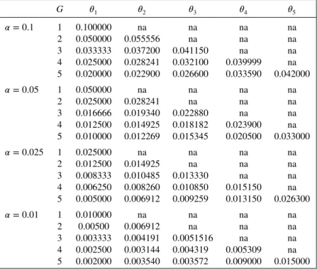
The tuning parameter𝜃jis established such that𝜋0,j ⩽ 𝛼j. Recall that hj =⌊𝜃j(xj−1+1)−1⌋; then 𝜋0,jis a nondecreasing function with respect to𝜃j. Thus, a trivial numerical procedure, like the bisection method, will always give a feasible solution for𝜃jgiven an arbitrary𝛼j. The idea is to find out the largest value of𝜃jfor which𝜋0,j ⩽𝛼j. Table I brings𝜃jsolutions for some common parameterization choices. The values in this table were obtained under a uniform alpha spending, that is, 𝛼j = 𝛼∕G, where 𝛼 is the overall desired significance level. The solutions were possible through the bisection method and
Table I.Threshold settings to use the Monte Carlo alpha spending for global significance levels of𝛼=0.1,0.05,0.025,0.01,m=999, andG=1,…,5.
G 𝜃1 𝜃2 𝜃3 𝜃4 𝜃5
𝛼=0.1 1 0.100000 na na na na
2 0.050000 0.055556 na na na
3 0.033333 0.037200 0.041150 na na
4 0.025000 0.028241 0.032100 0.039999 na
5 0.020000 0.022900 0.026600 0.033590 0.042000
𝛼=0.05 1 0.050000 na na na na
2 0.025000 0.028241 na na na
3 0.016666 0.019340 0.022880 na na
4 0.012500 0.014925 0.018182 0.023900 na
5 0.010000 0.012269 0.015345 0.020500 0.033000
𝛼=0.025 1 0.025000 na na na na
2 0.012500 0.014925 na na na
3 0.008333 0.010485 0.013330 na na
4 0.006250 0.008260 0.010850 0.015150 na
5 0.005000 0.006912 0.009259 0.013150 0.026300
𝛼=0.01 1 0.010000 na na na na
2 0.00500 0.006912 na na na
3 0.003333 0.004191 0.0051516 na na
4 0.002500 0.003144 0.004319 0.005309 na
5 0.002000 0.003540 0.003572 0.009000 0.015000
Here, the alpha spending used for each group testing is𝛼j=𝛼∕G.
implemented in the R software [17]. This table was built form = 999, and the solutions for largerm values will differ only slightly in a way that does not affect the significance level in each test. Thus, the values shown in this table can be used for larger values ofmsuch as 9999 or 99,999.
The uniform alpha spending is a simple and intuitive choice for cases where the analyst has no practical concerns about the statistical performance of the analysis besides the global level of the sequential test. But, the Monte Carlo procedure introduced in this section is actually advantageous when the analyst indeed desires to establish a personalized, and maybe uncommon, alpha spending function. Many shapes can be designed for the alpha spending function given a maximum numberGof tests and an overall𝛼 level, and it depends on each problem according to financial, logistical, or ethical issues. For example, suppose that forG=5 and𝛼=0.05, the desired alpha spending is to be managed in the following way: 𝛼1 =0.02,𝛼2 =0.015,𝛼3 =0.01,𝛼4 =0.003, and𝛼5 =0.002. In this setting, the associated thresholds are𝜃1=0.02,𝜃2 =0.01767,𝜃3=0.015345,𝜃4=0.0096, and𝜃5 =0.0085.
3.2. Statistical power performance
The variability introduced by the Monte Carlo approach can lead to reductions in terms of statistical power with respect to the theoretical exact sequential test. This section develops an analytical expression to bound such potential power losses. This is possible by assuming a regular class of probability distributions for the exact conditionalp-value.
3.2.1. A class of distributions for the conditional p-value. By definition, the exact conditionalp-value, expression (7), is a random variable. In order to study the performance of the sequential Monte Carlo test, Fay and Follmann [18] introduced a class ofp-value distributions with shape of the form
H𝛼,1−𝛽(p) =1− Φ
{
Φ−1(1−p) − Φ−1(1−𝛼) + Φ−1(𝛽)}, (15)
whereΦ(.)is the cumulative distribution function of a standard normal distribution and𝛽is the type II error probability. The rationale behind the use of this class is that among the possible real scenarios where (15) holds, one can find out regular distributions families like the cases where the test statistic either follows the standard normal distribution under the null hypothesis and anN(𝜇,1)under the alternative, or a central𝜒(2)
1 under the null hypothesis and a noncentral𝜒 (2)
1 under the alternative hypothesis.
If the power function of a Monte Carlo test design is nonincreasing withp, the greatest power loss occurs when𝛽is equal to 0.5, that is, the worst case isH𝛼,0.5(p). To see this, leth(p)be a probability
density function related to a member inside this class. Indexed by𝛼and𝛽, a particular member of this class is related to the following probability density function:
h𝛼,1−𝛽(p) =exp
{
−1
2 [
Φ−1(𝛽) − Φ−1(1−𝛼)] [Φ−1(𝛽) − Φ−1(1−𝛼) +2Φ−1(1−p)]}, (16)
whereΦ−1is the inverse function of the standard normal cumulative distribution functionΦ(⋅). The first
derivative ofh𝛼,1−𝛽(p)with respect topis equal to
h′𝛼,1−𝛽(p) =
[
Φ−1(𝛽) − Φ−1(1−𝛼)]
𝜙Z(Φ−1(1−p)) h𝛼,1−𝛽(p), (17)
where𝜙Z(⋅)is the density function of the standard normal distribution. For 1−𝛽⩾𝛼, we haveh′𝛼,1−𝛽(p)⩽
0 for allp∈ (0,1). If, for a fixedp, the Monte Carlo test is decreasing withp, then the worst case probabil-ity distributionH𝛼,1−𝛽(p)is the one that maximizesh𝛼,1−𝛽(p)forp=𝛼; that is, the evaluation of the worse is made by finding out the𝛽value that maximizesh𝛼,1−𝛽(𝛼) =exp
{
−0.5[(Φ−1(𝛽))2−(Φ−1(1−𝛼))2]}
with respect to𝛽. Observe that because of the symmetry property of the normal distribution, the mini-mum value of(Φ−1(𝛽))2occurs for𝛽=0.5 becauseΦ−1(0.5) =0; then, for any𝛼⩽1−𝛽, the analytical
solution that maximizesh𝛼,1−𝛽(𝛼), with respect to𝛽, is𝛽=0.5.
3.2.2. Upper bounds for potential power losses. Assume that the conditional probability distribution of Pk, givenPk−1,…,P1, represented byFP
k−, is shaped according to (15). This assumption is adequate, for
example, for the cases whereUj is a Markovian stochastic process, that is, the conditional distribution ofUj, given the pass, only depends on the observed statistic of the immediately predecessor test. Under these terms, it seems to be reasonable to assume that the same family of distribution is adequate for each of the conditional distributions.
The function𝜋k(p1,…,pk),k ⩽ G, is decreasing withpk and, forj <k,𝜋k(p1,…,pk)is increasing withpj. Recall that if the Monte Carlo power function for thekth test is decreasing with pk, then the worst distribution scenario of the type (15) occurs for𝛽 =0.5. If(1−𝛽)⩾𝛼, because𝜋k(p1,…,pk)is increasing withpj (j <k) and, from expression (17),h𝛼,1−𝛽(p)is nonincreasing withp, the worst case
in thekth test forFP
j−, withj <k, is the uniform(0,1) distribution. But, the analytical manipulation of
the Monte Carlo power by usingH𝛼,1−𝛽(p)is intractable. To circumvent this problem, and following the
suggestion from Fay and Follmann [18], aBeta(a,b)distribution can be used to approximateH𝛼,1−𝛽(p).
Denote this approximating function byH̃𝛼;0.5(p). This approximation is chosen in a way that the expected
value ofpcoincides with that fromH𝛼,1−𝛽(p), andH̃𝛼,1−𝛽(𝛼) =H𝛼,1−𝛽(𝛼) =1−𝛽. Thus, a lower bound,
𝜋∗
k, for the power of thekth Monte Carlo test, is given by
𝜋∗k = m
∑
x1=h1+1
x1
∑
x2=h2+1
· · · xj−2
∑
xk−1=hk−1+1
hk ∑
xk=0 Cxk−1
xk B(a+xk,b+xk−1−xk) B(a,b)∏kj=−11(xj+1)
. (18)
For evaluating the power difference between the Monte Carlo and the exact approaches, it is helpful to obtain the expression for the exact power of the kth test, denoted here by 𝛽A,k, and which can be expressed by
𝛽A,k=∫ 1
𝜙1 ∫
1
𝜙2
· · ·∫ 1
𝜙k−1∫ 𝜙k
0
̃
H𝛼;0.5(p)dp=FH(𝜙k|a,b) k−1
∏
j=0
(1−𝜙j), (19)
where𝜙0 =0,FH(𝜙k|a,b)is theBeta(a,b)distribution evaluated at𝜙k, and𝜙1,…, 𝜙kare chosen in a way to ensure the desired alpha spending for thekth test. Thus, from (18) and (19), an upper bound for the power loss of the proposed Monte Carlo design is as follows:
max
k
{
𝛽A,k−𝜋k∗}. (20)
Let𝛽0,kbe the type I error probability in thekth test, which is obtained by integrating the multivariate uniform(0,1)kdensity, in the rejection region, for thekth test. Fork= 1 and for an alpha spending of
𝛼1, the value of𝜙1is𝛼1. Fork=2,
𝛽0,2 =∫ 1
𝜙1 ∫
𝜙2
0
dp2dp1=𝜙2(1−𝜙1) =𝜙2(1−𝛼1),
⇒for an alpha spending of𝛼2, we have𝜙2 =𝛼2∕(1−𝛼1).
By recursive application of the previous reasoning, the alpha spending at thekth test, fork=1,· · ·,G, is given by
𝛽0,k=∫ 1
𝜙1 ∫
1
𝜙2
· · ·∫ 1
𝜙k−1∫ 𝜙k
0
dpk· · ·dp1 =𝜙k
k−1
∏
i=0
(1−𝜙i). (21)
Then, if𝛼kis the alpha spending in thekth test, the value of𝜙kis explicitly obtained:
𝜙k=( 𝛼k
1−∑ki=−01𝛼i−1
), (22)
with𝛼0=0.
For the special case of a constant alpha spending, that is,𝛼j=𝛼∕G=𝜙, and from expression (21), the tuning parameters𝜙jare given by
𝜙j=𝜙− (j−1)𝜙2, forj=1,· · ·,G. (23)
Each combination of𝛼andGleads to a particular𝜙value, which, by its turn, leads to particular values ofaandbto be used in the approximating distributionH̃
𝛼,1−𝛽(p). For example, for𝛼=0.05 andG=1,
the associated solution isa=0.359 andb=2.523, which gives an upper bound for the power loss equal to 0.0187. ForG=5 and𝛼j =𝛼∕5, the solution isa=0.3 andb=7.6, which gives a power loss upper bound of 0.018.
IfUjis computationally hard to obtain, a sequential strategy can be adopted in order to save execution time in each single Monte Carlo test. Complicated calculation as, for example, those involved in lengthy inferential procedures usually leads to the situation where the test statistic distribution is unknown and Monte Carlo is required. For example, the multivariate problem of finding spatial clusters of disease outbreak requires the use of computationally intensive testing procedures, like the flexibly shaped scan statistic proposed by Tango and Takahashi [19]. The execution time of the flexibly shaped scan can take as long as 2 weeks depending on the application. Another example is the tree-based scan statistic for database disease surveillance proposed by Kulldorffet al. [20], which allows for the study of relation among many databases related to a sort of potential risk factors, and then it can take a long time to run. Computational speed is an important issue even today after the many advances in processing speed of computational resources. The big data analysis is an example of why saving execution time in numerical intensive procedures is still important. The next section is devoted to construct a method for perform-ing sequential Monte Carlo tests in sequential analysis. The method favors to save execution time in computational intensive problems that might appear in practice.
4. On a composite approach: sequential Monte Carlo for sequential analysis
The composite sequential procedure introduced in this section is indicated for applications where compu-tational time is a relevant issue. As already stressed earlier, the term ‘composite’ was chosen to emphasize that the method is a sequential procedure because of two different reasons: for each test, among a sequence ofGtests, a sequential Monte Carlo test is considered. There is a lack in the literature concerning a com-prehensive method of performing sequential Monte Carlo tests in the sequential analysis context. This composite scenario has already been treated by Jennison [21], but his proposal was concerned only on saving execution time in a single test. The problem of how to ensure the overall nominal significance level after multiple sequential Monte Carlo tests remains an open question. This section introduces a procedure to address this challenge. For thekth sequential test, define
Xt,k= t
∑
i=1
I{⋂k k=1Uk,i⩾uk
}(U
1,i,· · ·,Uk,i), (24)
which is the random variable to be tracked in thekth test after the tth simulation. Now, the concept of sequential risk introduced in Section 2.2 is extended for the sequential analysis context. Forc0,t =
min{⌊𝜃k(xt,k−1+1)⌋−1,t}andy0,t =min{⌊𝜃k(xt,k−1+1)⌋−1−x,xt,k−1−t}, the upper and the lower conditional sequential risks are defined by
CRu(t,k) = c0,t ∑
x=xt,k
y0,t ∑
y=0
Cxt,k−1
y CtxB(x+y+1,xt,k−1−x−y+1), and (25)
CRl(t,k) = xt,k
t+1−
x∑t,k−1
x=0 y0,t ∑
y=0
Cxt,k−1−1
y CtxB(x+y+1,xt,k−1−x−y+1), (26)
wherext,k−1is the observed value ofXt,k−1fork =1,· · ·,G, withxt,0 =t. The optimalMCo procedure
described in Section 2.2 can be applied in order to save execution time in thekth test. The power loss from such approach is not greater than 1%. The Monte Carlo simulation for thekth test is interrupted as soon as the decision function,𝜓t,k, is equal to 1 or 2. The null hypothesis is not rejected if𝜓t,k=1, and H0is rejected if𝜓t,k=2, where
𝜓t,k=
⎧ ⎪ ⎨ ⎪ ⎩
0, ifCRu(t,k)> 𝛿u,CRl(t,k)> 𝛿l,kandt<m, 1, ift>20 andCRu(t,k)⩽𝛿u,
2, ifCRl(t,k)⩽𝛿l,kor ift=m,
(27)
with𝛿u=0.01∕mand𝛿l,k=0.001∕⌊𝜃k(m+1)⌋. The threshold𝜃kis chosen in a way to ensure the desired alpha spending,𝛼k. Ift∗is the number of simulations at the interruption moment, a valid conditional sequentialp-value, for thekth sequential test, is given by
̄ Pk=
{X
t∗,k∕t∗, if𝜓t∗,k=1, (
Xt∗,k+1 )
∕(t∗+1), if𝜓t∗,k=2.
(28)
5. Monitoring adverse events after vaccination
The composite sequential method is illustrated here through an application for real data. This application is meant to mimic a post-market vaccine safety surveillance analysis, and the test statistic adopted is the cMaxSPRT statistic.
5.1. Data description
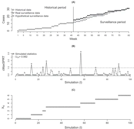
This illustrative example uses a time series data of health insurance claims from the Centers for Disease Control and Prevention-sponsored Vaccine Safety Datalink project. The series has 82 weekly entries, where each entry counts the number of adverse events associated with neurological symptoms within 28 days after Pediarix vaccination, which is manufactured by GlaxoSmithKline. This vaccine, with a simple injection, protects children from five different diseases: diphtheria, tetanus, whooping cough, hepatitis B, and polio. Figure 1(A) shows the time series formed by these 82 observed counts of adverse events indexed by week.
Recall that the cMaxSPRT requires the existence of a historical data. Once the objective here is not actually to analyze this data set but to use it as a realistic scenario to illustrate the applicability of the com-posite sequential approach, the data set was divided in two subsamples, each with 41 entries, where the first batch of 41 observations is taking as the historical sample and the second subsample as the surveil-lance sample. The surveilsurveil-lance sample is represented with the dark down triangles shown in Figure 1(A). Because these both samples came from the same population under the same vaccination, it is natural to expect that a test forH0 ∶𝜆V =𝜆PagainstH1∶𝜆V < 𝜆Pmay not reject the null. We use this controlled application as a motivation to verify if the data presented some change with respect to the relative risk
Figure 1.Real and hypothetical scenarios for the observed cMaxSPRT statistics at the fifth sequential test (A). The first hundred simulated values under the null (B) and theXl,5trajectory (C) are also available.
of having an adverse event during the weeks. An abrupt change in the cumulative cases occurred around 42nd week, and then it can be of interest to test if the relative risk after that point is increased.
5.2. Tuning parameters settings
The assumption of a Gamma distribution for Pk implies an exponential distribution, with mean 𝜆P, for each arrival time of thekindependent adverse events. Because the distribution of the ratioPk∕V, underH0, does not depend on 𝜆P, thetth Monte Carlo value from the null distribution ofUk can be obtained by generatingkindependent values from an exponential distribution with parameter 1∕𝜆P=1. The sum of such generated values represents the tth Monte Carlo cumulative person time (Pt,k) for the surveillance period. Similarly, the sum ofc independent values from an exponential distribution, with parameter 1∕𝜆V = 1, represents the tth Monte Carlo cumulative person time (Vt) for the his-torical data. The values Pt,k and Vt are then used to calculate thetth Monte Carlo copy (Ut,k) of the
cMaxSPRT statistic.
The analysis considers a scenario with a maximum of five tests (G = 5) and an overall signifi-cance level of 0.05 (𝛼 = 0.05). To further explore the flexibility offered by the Monte Carlo method in which concerns the management of the type I error, instead of a simple uniform function, here, the non-naive alpha spending of the end of Section 3.1 is considered:𝛼1 = 0.02,𝛼2 = 0.015,𝛼3 = 0.01, 𝛼4 = 0.003, and𝛼5 = 0.002, which leads to the thresholds𝜃1 = 0.02,𝜃2 =0.01767,𝜃3 = 0.015345, 𝜃4 = 0.0096, and 𝜃5 = 0.0085. Each test presents less than 1% of power loss; then the overall power loss is bounded at 5%. For this application, m = 100,000 and the threshold parameters are fixed according to Table (I). For the group sequential design, assume that a test is to be performed after each chunk of four adverse events, which means that the maximum length of surveillance is K=20.
5.3. Data analysis results
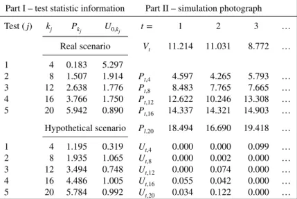
In the historical data, it was observed a total ofc = 11 adverse events accumulated afterv = 5.3415 (observedV) person-time amount. Observed values ofPk andU0,k
j,j = 1,…,5, are presented in the
Table II.Part I of this table gives the real and hypothetical scenarios for the observed cMaxSPRT statistics at each of the five sequential tests; part II shows the three first simulated cMaxSPRT values, underH0, for the
sequential analysis over the hypothetical data.
Part I – test statistic information Part II – simulation photograph
Test(j) kj Pk
j U0,kj t= 1 2 3 …
Real scenario Vt 11.214 11.031 8.772 …
1 4 0.183 5.297
2 8 1.507 1.914 Pt,4 4.597 4.265 5.793 …
3 12 2.638 1.776 Pt,8 8.483 7.765 7.665 …
4 16 3.766 1.750 Pt,12 12.622 10.246 13.308 …
5 20 5.942 0.890 Pt,16 14.337 14.321 14.903 …
Hypothetical scenario Pl.20 18.494 16.690 19.418 …
1 4 1.195 0.319 Ut,4 0.000 0.000 0.099 …
2 8 1.935 1.065 Ut,8 0.000 0.002 0.000 …
3 12 3.494 0.748 Ut,12 0.000 0.074 0.000 …
4 16 4.486 1.005 Ut,16 0.055 0.042 0.000 …
5 20 5.784 0.992 Ut,20 0.034 0.122 0.000 …
The historical information used here arec=11 andv=5.3415.
upper block (real scenario) of Table II, part I. The first four adverse events concentrated in a short person-time amount, equal to 0.183. This high frequency is reflected through a large observed value ofU0,4 =
5.297, which is the observed test statistic for the first group sequential test (j=1). This result indicates that there may exist an inflation in the relative risk at some point after the last cases observed in the historical period.
The first group sequential test (j =1) is based on the Monte Carlo simulationsU1,4,U2,4, and so on. For the calculations shown in this example, the simulations were possible by generating random numbers from an exponential distribution through the ‘rexp’ function of the R software. The simulated values were then combined in order to form theUt,4according to the instructions given in the first paragraph of
Section 5.2. TheMCosignaling thresholds,𝛿uand𝛿l,4, were not touched beforet =99,999 in this first test, and the observedp-value was equal to 566∕100,000=0.00566 (x99999,4 =565). Thus, because the
observedp-value is smaller than the threshold𝜃1 =0.02,H0 is to be rejected; that is, for a significance level of 0.02, we should conclude that𝜆Pis greater than𝜆V.
From a practical perspective, the analyst should stop the sequential surveillance and conclude thatH0 is to be rejected. However, in order to further explore this application, fake data showing a different line shape are considered for the surveillance period. The trajectory of this new series of cumulative cases is represented with the symbol ‘×’ in Figure 1(A) in the surveillance period. Note that the jumping after week 41 is not present in this fake series. The summary for the observed statistics from these new data is offered in the lower block (hypothetical scenario) of Table II, part I. To help with the understanding behind each step in this composite sequential analysis, Table II also presents, in part II, the first three Monte Carlo cumulative person-time values for both historical (Vt) and surveillance (Pt,kj) periods, as well as the relatedUt,k
j. This information is used to obtainXt,j. For example, withj=1, theXt,1value is obtained by comparing the line labeled asUt,4with the first value, 0.319, of the Hypothetical scenario of
Table II.
For the first test (k1 = 4),CRu(t,k)turned out smaller than 𝛿u = 0.01∕99,999 = 10−7 just after
the 20-s simulated statistic, which returnedx22,1 = 6, leading to ap-value ofp̄1 =x22,1∕t∗ = 6∕22 ≈
0.273. Thus,H0was not rejected at the first group sequential test. For the second test (k2 =8),CRu(t,k)
turned out smaller than 10−7after the ninth simulated statistic withx
31,2=4. The observedp-value was
̄
p2 = (x31,2)∕(x22,1+9) = 4∕(15) =≈ 0.267. Tests number three (k1 = 12), four (k1 = 16), and five
(k1 =20) also crossed the threshold(𝛿u = 10−7)before the simulation of number 99,999. Then,H 0is
not rejected with these fake data. Figure 1(B) shows the trajectory for the first hundred simulated values U1,20,U2,20,…,U100,20. These values are used in the fifth sequential test (j=5). Figure 1(C) presents the
values ofXt,5 =
∑t
i=1I(Ut,20⩾0.992)while it evolves witht.
6. Conclusions
Monte Carlo simulation was demonstrated to be a feasible approach for sequential analysis. The true control of the type I error probability associated with a sequence of tests is guaranteed. More importantly, such control is valid for any statistical dependence structure among the distributions of the test statistics calculated in each look at the data. Although inspired by the post-market vaccine safety surveillance problem, the method can be directly applied for sequential analysis of any other sort of problem. The real application shown in this paper is not an example of computationally intensive problem. The evaluation of the real gains with the composite design, in terms of expected signal time, should be explored for time-consuming statistical tools, such as the tree-based scan statistic for database disease surveillance. This is a lack left for future studies.
Acknowledgements
This research was funded by the National Institute of General Medical Sciences, USA, grant #RO1GM108999. Additional support was provided by Fundação de Amparo à Pesquisa do Estado de Minas Gerais, Minas Gerais, Brasil (FAPEMIG).
References
1. Lieu T, Kulldorff M, Davis R, Lewis E, Weintraub E, Yih W, Yin R, Brown J, Platt R. Real-time vaccine safety surveillance for the early detection of adverse events.Medical Care2007;45(S):89–95.
2. Klein NP, Fireman B, Yih WK, Lewis E, Kulldorff M, Ray P, Baxter R, Hambidge S, Nordin J, Naleway A, Belongia EA, Lieu T, Baggs J, Weintraub E, Vaccine Safety Datalink. Measles-mumps-rubella-varicella combination vaccine and risk of febrile seizures.Pediatrics2010;126:e1–e8.
3. Avery T, Vilk Y, Kulldorff M, Li L, Cheetham T, Dublin. S. Prospective, active surveillance for medication safety in population-based health networks: a pilot study.Pharmacoepidemiol Drug Saf2010;19:S304.
4. Belongia EA, Irving SA, Shui IM, Kulldorff M, Lewis E, Yin R, Lieu TA, Weintraub E, Yih WK, Li R, Baggs J, Vaccine Safety Datalink Investigation Group. Real-time surveillance to assess risk of intussusception and other adverse events after pentavalent, bovine-derived rotavirus vaccine.Pediatric Infectious Disease Journal2010;29:1–5.
5. Yih W, Nordin J, Kulldorff M, Lewisc E, Lieua T, Shia P, Weintraube E. An assessment of the Safety Datalink of adolescent and adult tetanus-diphtheria-acellular pertussis (TDAP) vaccine, using active surveillance for adverse events in the Vaccine Safety Datalink.Vaccine2009;27:4257–4262.
6. Silva I, Assunção R, Costa M. Power of the sequential Monte Carlo test.Sequential Analysis2009;28(2):163–174. 7. Li L, Kulldorff M. A conditional maximized sequential probability ratio test for pharmacovigilance.Statistics in Medicine
2010;29:284–295.
8. Pocock S. Group sequential methods in the design and analysis of clinical trials.Biometrika1977;64:191–199. 9. O’Brien P, Fleming T. A multiple testing procedure for clinical trials.Biometrics1979;35:549–556.
10. Kulldorff M, Davis RL, Kolczak M, Lewis E, Lieu T, Platt R. A maximized sequential probability ratio test for drug and vaccine safety surveillance.Sequential Analysis2011;30:58–78.
11. Jennison V, Turnbull B.Group Sequential Methods with Applications to Clinical Trials. Chapman and Hall/CRC: London, 1999. ISBN 0-8493-0316-8.
12. Dwass M. Modified randomization tests for nonparametric hypotheses.Annals of Mathematical Statistics 1957;28: 181–187.
13. Barnard GA. Contribution to the discussion of professor Bartlett’s paper.Journal of the Royal Statistical Society1963;
25B:294.
14. Hope A. A simplified Monte Carlo significance test procedure.Journal of the Royal Statistical Society1968;30B:582–598. 15. Birnbaum ZW. Computers and unconventional test statistics. InReliability and Biometry: Statistical Analysis of Lifelength,
5th ed., Proschan F, Serfling RJ (eds). Soc. Indust. Appl. Math.: Philadelphia, 1974; 441–458.
16. Silva I, Assunção R. Optimal generalized truncated sequential Monte Carlo test.Journal of Multivariate Analysis2013;
121:33–49.
17. Team RC. R: a language and environment for statistical computing.R Foundation for Statistical ComputingVienna, Austria 2014. http://www.R-project.org [Accesses on 18 November 2014].
18. Fay M, Follmann D. Designing Monte Carlo implementations of permutation or bootstrap hypothesis tests.The American Statistician2002;56(1):63–70.
19. Tango T, Takahashi K. A flexibly shaped spatial scan statistic for detecting clusters.International Journal of Health Geographics2005;4:4–11.
20. Kulldorff M, Fang Z, Walsh S. A tree-based scan statistic for database disease surveillance.Biometrics2003;59:323–331. 21. Jennison C. Bootstrap tests and confidence intervals for a hazard ratio when the number of observed failures is small, with
applications to group sequential survival studies.Computing Science and Statistics1992;22:89–97.