A critical analysis of the Caputo-Fabrizio operator
Manuel D. Ortigueiraa, J. Tenreiro MachadobaUNINOVA and DEE of Faculdade de Ciˆencias e Tecnologia da UNL
Campus da FCT da UNL, Quinta da Torre, 2829 – 516 Caparica, Portugal (e-mail: [email protected])
bInstitute of Engineering, Polytechnic of Porto, Dept. of Electrical Engineering, R. Dr. Ant´onio Bernardino
de Almeida, 431, 4249-015 Porto, Portugal (e-mail: [email protected])
Abstract
This short note analyses the Caputo-Fabrizio operator. It is verified that it does not fit the usual concepts neither for fractional nor for integer derivative/integral.
Keywords: Fractional derivative, Caputo-Fabrizio operator.
1. Introduction
In recent years, several operators were proposed having the keyword “fractional”. One of the proposals consists of the Caputo-Fabrizio (CF) operator [1] that is defined by the expression
D(↵)t f (t) =M (↵)
1 ↵
Z t a
f0(⌧ )e 1↵↵(t ⌧ )d⌧, (1)
where 0 ↵ 1, a 2 ( 1, t) and M(↵) is a normalization function such that M(0) = M(1) = 1. We will assume that (1) is valid for functions having Laplace transform (LT).
In the following we analyse this operator and we verify that it implements an integer order highpass filter. We can prove that the CF operator is neither fractional, nor a derivative, by showing that it does not verify the Leibniz rule [11]. The proof is somehow involved and we shall adopt here a di↵erent perspective based on Laplace transform and Bode diagrams.
2. The analysis
2.1. Is the CF operator fractional?
Let us consider expression (1) and a = 0 just in order to simplify expressions. Recalling that the multiplication of 2 Laplace transforms corresponds to the convolution in the time domain, equation (1) can be written as
g(t) = D(↵)t f (t) =M (↵) 1 ↵f
0(t)⇤⇥e ↵
1 ↵t"(t)⇤, (2)
*Manuscript
where "(t) stands for the Heaviside unit step and⇤ denotes the convolution. The bilateral Laplace transform (no initial conditions are needed [9]) of (2) gives
G(s) =M (↵) 1 ↵ s s + ↵ 1 ↵ F (s), (3)
where F (s) = L[f (t)] and G(s) = L[g(t)]. Equation (3) can be interpreted as an input/output relation of a linear system with transfer function given by [8, 9]
H(s) =M (↵) 1 ↵ s s + ↵ 1 ↵ . (4)
Therefore, the operator has a transfer function with one zero at s = 0 and one pole at s = ↵
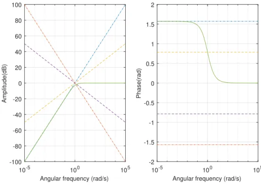
1 ↵. The region of convergence is given by Re(s) > 1 ↵↵ , that includes the imaginary axis. Considering s = i!, i =p 1, !2 R, we obtain the frequency response, H(i!), namely the amplitude and phase spectra, and we can plot the corresponding Bode diagrams. Figure 1 presents the Bode plots for ↵ = 0.5. For comparison, we joined the plots corresponding to H(s) = s↵ with ↵ =±0.5, ±1. We observe that the CF operator:
10-5 100 105
Angular frequency (rad/s) -100 -80 -60 -40 -20 0 20 40 60 80 100 Amplitude(dB) 10-5 100 105
Angular frequency (rad/s) -2 -1.5 -1 -0.5 0 0.5 1 1.5 2 Phase(rad)
Figure 1: Bode plots of Amplitudes and Phases for the normalised CF operator, 2M (0.5)|G(i!)|, that are represented by continuous lines, and for derivatives and integrals, represented by straight lines corresponding to the orders±1 (dash-dash) and ±0.5 (dot-dash).
• is a highpass filter.
• has an amplitude spectrum that increases 20dB/dec till ! = ↵
1 ↵ and then stabilises. Therefore, the slope is 20dB/dec at low frequencies and 0 dB/dec at high frequencies. • The phase varies from ⇡/2 to 0 radians.
In summary, the derivatives and integrals are represented by straight lines. Nevertheless, we verify that the frequency response of CF operator is not fractional, since neither the left nor the right slopes in the amplitude diagram are ↵· 20dB/dec and the phase diagram is not ↵ · ⇡/2 [5]. This conclusion is based on (i) the adoption of Laplace transform and its properties and (ii) the assumption that both fractional and integer derivatives have a representation by straight lines in Bode diagrams. While this approach does not follow the classical analytical derivations, it shows that we can adopt well established tools of applied sciences.
2.2. Is the CF operator a derivative?
Let us return to expression (3) and rewrite it as
[(1 ↵)s + ↵] G(s) = M (↵)sF (s). With the inverse LT, we obtain
(1 ↵)Dg(t) + ↵g(t) = M (↵)Df (t), (5)
where D represents the derivative of order one. If ↵ = 1, then the operator is a derivative, but not fractional. If ↵6= 1, then the operator is not a derivative. Equation (5) is standard in linear systems and describes the input/output of a highpass filter [3]. Therefore, we conclude that the CF operator is not a derivative.
We adopted the Fourier analysis in the previous calculations, but, in fact, we can also justify these results by applying the criteria proposed in [7]. Operator (1) does not verify all the requirements and in particular we can verify that
D↵tDtf (t)6= D↵+t f (t), ↵, < 1. (6) Let us consider (3) and assume that ↵6= . We can write
LnD↵tDtf (t) i = M (↵) 1 ↵ M ( ) 1 s s + ↵ 1 ↵ s s +1 F (s). Since we have s ⇣ s + ↵ 1 ↵ ⌘ ⇣ s +1 ⌘ = ↵(1 ) (1 ↵) s + ↵ 1 ↵ + (1 ↵) ↵(1 ) s +1 ,
then LnD↵ tDtf (t) i = ( ↵M ( ) (1 ↵) " M (↵) 1 ↵ s s +1 ↵↵ # M (↵) ↵(1 ) " M ( ) 1 s s +1 #) F (s). (7) Therefore D↵
tDtf (t) is expressed as a linear combination of D↵tf (t) and Dtf (t). On the other hand, substituting ↵ + in (3) we get
LnD↵+t f (t)i=M (↵ + )
1 ↵
s
s +1 ↵↵+ F (s). (8)
Since expressions (7) and (8) are distinct we prove (6).
2.3. A generalised fractional CF operator
In the same line of ideas underlying the CF operator, Atangana and Baleanu [2] proposed the substitution of the exponential in (1) by the Mittag-Le✏er function
E↵(t) = 1 X k=0 pk tk↵ (k↵ + 1)"(t), t2 R, (9) with p = ↵
1 ↵. Such operator assumes the form
D(↵)t f (t) = M (↵) 1 ↵ Z t a f0(⌧ )E↵ ↵ 1 ↵(t ⌧ ) ↵ d⌧. (10)
Using the LT of the Mittag-Le✏er function L [E↵(t)] = s
↵ 1
s↵ p [4], we derive the transfer function of the generalised operator
H(s) =M (↵) 1 ↵ s↵ s↵+ ↵ 1 ↵ . (11)
The corresponding di↵erential equation becomes
(1 ↵)D↵g(t) + ↵g(t) = M (↵)D↵f (t), (12)
where L[D↵g(t)] = s↵G(s) [8]. The operator may be called fractional, but it is not a derivative.
3. Conclusions
The analysis of the Caputo-Fabrizio operator revealed that it is neither a fractional nor a derivative operator [6]. Similarly, the generalization of the operator is not a fractional derivative. In this short note was adopted a strategy based on Laplace transform and related properties. The results support the use in FC of mathematical tools well established in the area of applied sciences.
Acknowledgement
This work was partially funded by National Funds through the Foundation for Science and Technology of Portugal, under the projects PEst-UID/EEA/00066/2013.
Conflict of Interest
The authors declare that they have no conflict of interest.
References
[1] Caputo, M. and Fabrizio, F., A new Definition of Fractional Derivative without Singular Kernel, Progr. Fract. Di↵er. Appl. 1, No. 2, 73–85 (2015).
[2] Atangana, A. and Baleanu, D., New Fractional Derivatives with Local and Non-Singular Kernel: Theory and Application to Heat Transfer Model, Thermal Science, 20, 763–769, (2016).
[3] Dorf, R.C. and Svoboda, J.A., Introduction to Electric Circuits, 9th Edition International Student Version, Wiley, 2013.
[4] Kilbas, A. A., Srivastava, H. M. and Trujillo, J. J. Theory and Applications of Fractional Di↵erential Equations, Elsevier, Amsterdan, 2006.
[5] Machado, J.A.T., Fractional derivatives: Probability interpretation and frequency response of rational approximations, Communications in Nonlinear Science and Numerical Simula-tion, Volume 14, Issues 9-10, pp 3492–3497, 2009.
[6] Machado, J., Mainardi, F., Kiryakova, V., et al., Fractional Calculus: D’o`u venons-nous? Que sommes-nous? O`u allons-nous?, Fractional Calculus and Applied Analysis, 19(5), pp. 1074–1104, 2016.
[7] Ortigueira, M.D., Machado, J.T. What is a fractional derivative?, J. Comput. Phys., 293, 4–13, 2015.
[8] Ortigueira, M.D. Fractional Calculus for Scientists and Engineers, Lecture Notes in Elec-trical Engineering; Springer: Dordrecht, The Netherlands, 2011; Volume 84.
[9] Roberts,M. J., Signals and systems: Analysis using transform methods and Matlab, McGraw-Hill, 2003.
[10] Tarasov, V.E., Fractional Dynamics: Applications of Fractional Calculus to Dynamics of Particles, Fields and Media, Higher Eduaction Press, Beijing and Springer-Verlag Berlin Heidelberg, 2010.
[11] Tarasov, V.E., No violation of the Leibniz rule; No fractional derivative, Communications in Nonlinear Science and Numerical Simulation, Volume 18, pp. 2945-2948, 2013.