Age and gender classification: a proposed system

(1)

Department of Computer Science and Technology

Age and Gender Classification – A Proposed System

David Pereira da Silva

A Dissertation presented in partial fulfillment of the Requirements for the Degree of Master in Computer Engineering

Supervisors:

Doutor João Carlos Amaro Ferreira, Assistant Professor, ISCTE – IUL

Doutor Pedro Figueiredo Santana, Assistant Professor, ISCTE – IUL

(2)

(3)

iii

Acknowledgements

I would like to thank both my supervisors, Prof. João Carlos Amaro Ferreira and Prof. Pedro Figueiredo Santana, for all the guidance during this dissertation, without whom this work would not be possible. I am very grateful for all their support along this last year. Their input and ideas were definitely crucial and enabled me to enrich this thesis and finish it in a timely manner. I would also like to thank INOV for providing us with the dissertation theme that was aborded here. They provided us with the system requirements that they were envisioning and with the scope where such system would be applied.

(4)

(5)

v

Resumo

Com o aparecimento do Regulamento Geral de Proteção de Dados, têm surgido várias preocupações no que diz respeito ao armazenamento de dados sensíveis e pessoais de clientes. Com isto, surge a necessidade de obter informação sem guardar quaisquer dados sensíveis que possam identificar a pessoa aos quais dizem respeito. Um exemplo, que serviu de motivação para o trabalho desenvolvido nesta dissertação, é o de uma aplicação que requeira a criação de modelos que sejam capazes de recolher informação acerca do tipo de pessoas que frequenta determinadas áreas comerciais, utilizando os seus sistemas de vigilância como dados de entrada para essa aplicação.

No presente trabalho foi desenvolvido um sistema com o intuito de obter dados, nomeadamente a idade e género, através da utilização de imagens, utilizando para isso técnicas de Deep Learning. Este sistema é constuído por um modelo de detecção de pessoas baeado no modelo GoogLeNet e, para a classificação de idades e género, por uma Wide Residual Network, suportada por uma Rede Siamesa no que diz respeito à classificação de género. Para além da criação de um sistema capaz de classificar idades e género a partir de imagens de forma integrada, no melhor do nosso conhecimento, esse sistema constitui a primeira implementação disponível que utiliza Wide Residual Networks em conjunto com Redes Siameses para o problema específico da classificação de género.

Palavras-Chave: Detecção de Faces; Deep Learning; Redes Neuronais Convolucionais; Previsão de Género; Inteligência Artificial; Classificação por Idade

(6)

(7)

vii

Abstract

With the new General Data Protection Regulation, there has been a lot of concerns when it comes to saving personal and sensitive data. As a result, there is a necessity to gather information without storing any data that could be considered sensitive, and that could identify the person to which it belongs to. Our motivation was to create a system that could be used to gather information about the people that visit commercial areas, using their surveillance systems as input to the application.

In the present work, we developed a system capable of gathering age and gender information from people based on images, using Deep Learning. Such system was built using a face detection model based on the GoogLeNet deep neural network and on a Wide Residual Network for age and gender classification, supported by a Siamese Network for the latter. The outcome is, to the best of our knowledge, the first available implementation that makes use of Wide Residual Networks and Siamese Networks at the same time for gender classification.

Keywords: Face Detection; Deep Learning; Convolutional Neural Network; Gender Prediction; Artificial Intelligence; Age Classification

(8)

(9)

ix

Figure Index

Figure 1 - Example of a Convolutional Neural Network [28]. ...8

Figure 2- Siamese Network example [26]. ...9

Figure 3- One-shot Learning example [29]. ... 10

Figure 4- Diagram of the face detection model. ... 19

Figure 5- Final model workflow. ... 20

Figure 6- LBP cascade failed images sample. ... 24

Figure 7- MTCNN failed images sample. ... 24

Figure 8- One-Shot training data creation flow. ... 31

Figure 9- Age correctly predicted data. Left side image is the input image, while the right side image is the validation image to which the input was matched. ... 32

Figure 10- Age failed prediction data. Left side image is the input image, while the right side image is the validation image to which the input was matched. ... 32

Figure 11- Gender correctly predicted data. Left side image is the input image, while the right side image is the validation image to which the input was matched. ... 34

Figure 12- Gender failed prediction data. Left side image is the input image, while the right side image is the validation image to which the input was matched. ... 34

Figure 13- Gender failed prediction data. The left side images were wrongly annotated in the initial dataset and are the inputs, while the right side image is the validation image to which the input was matched. ... 34

Figure 14- False positives/negatives rate by image size. ... 36

Figure 15- Sample of a false positive. ... 37

Figure 16- Failed samples from class 1-9. Each bounding box is associated with the predicted age, followed by the annotated age. ... 42

Figure 17- Failed samples from class 60-101. Each bounding box is associated with the predicted age, followed by the annotated age. ... 42

Figure 18- Folder structure. ... 51

Figure 19- models folder content. ... 52

Figure 20- Classes.py file. ... 52

(12)

(13)

xiii

Table Index

Table 1- Face Detection studied papers. ... 14

Table 2- Age and Gender classification related papers. ... 16

Table 3- Comparison between face detection systems. ... 25

Table 4- Samples with the softmax probability distribution by class. ... 28

Table 5- Accuracy using different probability ranges (p stands for probability). ... 28

Table 6- Accuracy over ranking similarity for under-confident examples. ... 31

Table 7- Comparison using different confidences. ... 38

Table 8- Age confusion matrix.The values in bold represent the rate on correctly predicted data for each class... 39

(14)

(15)

xv

List of Acronyms

AFW – Annotated Faces in the Wild AI – Artificial Intelligence

BLOB - Binary Large Object

CNN - Convolutional Neural Networks DNN - Deep Neural Network

FDDB - Face Detection Dataset and Benchmark GDPR - General Data Protection Regulation IBM - International Business Machines LBP - Local Binary Pattern

MTCNN - Multi-Task Cascaded Convolutional Networks OpenCV - Open Source Computer Vision’s

RCNN - Region based CNN ReLU - Rectified Linear Units

(16)

1

1. Introduction

1.1. Motivation

With the approval of the General Data Protection Regulation (GDPR), the use of a client’s personal information has become very strict. Since currently, it is not legal to store a person’s sensitive information (name, email, phone number) without one's consent, there is a need to have an alternative way to gather clients information for marketing purposes. Such alternative ways include the use of artificial intelligence (AI) models that can make use of a client’s information to extract useful knowledge. The incremental evolution of AI models and their successes on specific tasks, such as visual recognition [3,4,5,7,8] and classification [6,9,11,12,13] problems, have presented a new way to solve complex issues. Such issues that have in the last years received an increasing amount of attention are age and gender classification problems. There have been multiple approaches that focus their work on achieving a high accuracy rate for this kind of predictions. Latest approaches commonly use Convolutional Neural Networks (CNN), as those have been presenting state-of-the-art results, although a number of limitations to this kind of networks reduce the progress that such models can achieve. One of the limitations of such systems is the increased amount of data required when training the model. The model’s accuracy rates depend not only on the implemented network but also on the data that is used to train it. The training data is what allows the system to learn to identify and predict outcomes correctly, therefore, the more data that is fed to the network, the better the results. Having large datasets to train a network is commonly a problem, as such datasets need to be labeled for the specific problem at hand and usually require an initial cleanup process before feeding it to the model. Another common problem, when it comes to face detection or age/gender classification, and usually one of the most important ones, are partial occlusions and low-quality images. Those influence directly the outcome results as the model has less information to work on, which makes it harder to predict. The same applies when it is a human making the prediction. If the image has low quality, it is harder for a human to be able to understand what is being seen, and therefore, to make a prediction.

(17)

2 1.2. Context

In our specific study case, the focus is to allow a supermarket to gather client statistics to make informed decisions, increase the quality of their service, and improve customer service. This is done making use of face recognition and age/gender classification algorithms applied over client’s images, which allows for such statistics to be generated.With this in mind, this research has the intent of creating a system which can efficiently detect and categorize people in images, identifying what their gender is and, given a set of pre-defined age classes, being able to predict in which one that person falls in.

One way to attain this is to use age and gender automatic, i.e., anonymized, classification methods. This can be achieved using neural networks, provided that these are able to produce high confidence predictions, i.e., relevant and trustworthy. Therefore, this project falls under the area of artificial intelligence (AI) since it uses Deep Learning models in order to extract information from images and make accurate predictions using those.

The proposed system works with the client’s images as input, using those to make the gender/age classifications and to, therefore, deliver that information to the users.

1.3. Research Questions Towards the Research Goals

There are a few questions that need to be answered, which will allow us to reach the goals that are proposed. Such questions are listed below:

 Which face detection models are publicly available and with satisfactory results?

 Which age and gender classification models are publicly available and with satisfactory results?

For our system to be built, we need to investigate which models are publicly available and which can be used by us. We should also have their source code publicly available in order to analyze it, in case we need to make customizations. Their results must be in line with the system requirements definition.

(18)

3

 Is there a system that does both face detection and age/gender classification, while allowing the user to edit the age classes to avoid re-training the network?

One of the goals that were established is for the users to be able to configure the age classes that they want to use in order to avoid re-training the network each time this needs to be done. With this in mind, and to avoid replicating something that already exists, we need to understand if there are already authors who implemented such a feature in one of their works.

 Is there something in common in the failed samples that could explain those wrong outputs?

There could be some common points between all the failing samples that could explain why those outputs are not accurate. If this is the case, understanding the underlying issues will enable us to identify possible solutions to increase the model's performance.

1.4. Goals

The main objective of this research work is to create an efficient system that is able to detect faces in images and to classify such faces based on age and gender. Thus, the goals below can be derived from this:

 The system should be able to detect faces in images;

 The system should be able to classify a face into a set of age and gender classes;

 The system should be configurable in terms of age classes used;

 Evaluate currently available models for both face detection and age/gender classification;

 Create a system integrating the identified best available models;

 Evaluate the failing outputs of the integrated models in order to find an underlying reasons for such failures;

(19)

4

 Adapt the system to overcome the identified failing outputs to improve the classification accuracy.

For the first goal to be considered complete, the system needs to be able, provided an image with people, to identify most faces correctly and provide good images as input to the next part of the system, which is the age and gender classification model.

For the second goal to be reached, we need an accurate approach to provide a good age and gender classification on the customers, so that we can have a high categorization accuracy. When it comes to age prediction, a high accuracy could be troublesome to achieve as even humans find it hard to predict the age of a person based on their facial characteristics alone; hence, in this case, a lower accuracy might be acceptable.

The third goal allows the user to have some control over which classes to use. So the system should allow the user to configure the age classes as he sees fit, without requiring to re-train the underlying model.

Due to the fact that AI systems have grown rapidly over the last years, there are multiple models that are capable of detecting faces and others capable of classifying faces by age and gender. Therefore, an analysis needs to be conducted in order to validate which ones achieve better results for our problem, enabling us to decide which models to use in our system.

Finally, an analysis of the outputs that are wrongly predicted needs to be done in order to understand why such failures occur. The objective of this is to, after understanding why such images tend to fail, find a possible solution and adapt the system to increase the accuracy further.

1.5. Investigation Methodology

To be able to understand how we could achieve our goals, an investigation was done to study what kind of methods and techniques were being applied by other authors to provide a model that could solve our proposed problem. The investigation regarding the literature review was done using several known platforms like Google Scholar, ACM Digital Library, and IEEE Digital Library.

A separate investigation was done for both face detection and age/gender classification tasks, analyzing separate papers for each of them. All the methods applied were analyzed as part of the specific paper, and the results achieved for each of the problems presented were extracted

(20)

5 and registered. With this, we were able to have a summary of performances achieved and which techniques were used so that we can make an informed decision on how to create our system. The scope was focused to only include research from 2015 onwards, although a few older documents were used as well. With this, we wanted to have only recent papers related to the specified subjects, since recognition models are improving and evolving at a fast pace, and what was used in the last decade may not be the best approach today. Furthermore, an additional investigation was done to find existing models that could be used for our own purposes and testings.

1.6. Document Structure

This document is structured into several parts. As an initial chapter, there is the Literature Review. This chapter focuses on investigating other authors work around this kind of classification problems as well as identifying core concepts required to understand the state-of-the-art networks used for such problems.

In the System Development chapter is described the system requirements, a macro design of the system’s architecture describing each module’s functionality and output, and the development work that is done in order to create the system. We present several available frameworks that can be used for both face detection and age and gender classification. Such frameworks are explored and evaluated in order to create our global model as they have features required by us. With this combination of components, we created the first available implementation that makes use of both Wide Residual Networks and Siamese Networks for gender classification, which has proved benefits.

The Testing and Evaluation chapter evaluates the system’s performance and does additional investigations on the results in order to understand how accuracy rates could be further increased. Such investigations included testing multiple image sizes and investigating if there are common characteristics between the failing images.

In the last part, the Conclusions, we present what was achieved with this work and make considerations for any future work that can be done.

In the Attachments, we present the final models' structure, and we also present a user guide to let the users know how to run the model and how to configure it.

(21)

(22)

7

2. Literature Review

For us to be able to build a system and choose which models/techniques to use, we need to know what is being used by other approaches with results that could satisfy our goals. First, we need to identify which approach is being used the most with satisfactory results: this is the case of Deep Learning, which is used across all recent papers we investigated, where all of them use, more specifically, Convolutional Neural Networks [2,3,4,5,6,7,8,9,11,12,13,21]. Deep learning has shown considerable improvements when compared to older algorithms, especially when processing images and videos, which covers problems like object detection, object recognition and speech recognition, which are areas where our theme falls into [1]. This explains why latest approaches are currently all adopting Deep Learning to solve these issues.

2.1. Deep Learning

Machine Learning is mainly used for object identification, classification problems, and prediction problems, and is divided into Supervised Learning and Unsupervised Learning. Deep learning can be described as a set of techniques used as part of Machine Learning, more specifically used in neural networks, which work with a set of layers, where the layers allow the data that is the input to the system to be decomposed and analyzed [1]; those layers are not specifically designed for each problem, but they are part of a generic procedure that is adaptable to multiple problem types. So the same network structure can be used in different problems. How the network is trained and which data is used is what will distinguish the behavior of such a model. In the past years, Deep Learning has shown many improvements on various tasks that were for many years hard to solve by other algorithms, showing better results in multiple studies compared to previous works [1]. Such tasks include problems where the input has a complex structure and cannot be easily learned by traditional artificial intelligence algorithms, such as image classification (where each image is represented as a pixel array) and speech recognition.

(23)

8 2.1.1. Convolutional Neural Network

Since 2012, with the ImageNet competition, that these networks are achieving better results in image classification than other algorithms, which made them since then the most used approach for all recognition and detection tasks, approaching almost the same results as human performance [1]. In this same contest, A. Krizhevsky et al. created a Convolutional Neural Network to classify images into a range of 1000 classes, attaining a test error rate of 15.3%, which was 11% better than the second-best entry in the competition [2].

Convolutional Neural Networks (CNN) are a type of neural network that generalizes better than previous neural networks (e.g., multi-layer perceptrons). CNN is designed to process data in the form of multiple arrays, passing the input between layers that extract the necessary features of the input and assign to those features calculated weights (filters) that will decide which are more important.

Figure 1 - Example of a Convolutional Neural Network [28].

Figure 1 depicts a typical architecture of a CNN, where the input image is fed into another layer and, then, the output of that layer is fed into the next ones. Each layer has a specific purpose. The Convolutional Layer is the one responsible for extracting features from the image (resulting in a feature map). It uses a set of filters to make computations over the initial vector and extract features from it, feeding the result to the next layer; this can be used, for example, to detect edges in images [14].

(24)

9 The Pooling layer reduces the dimensionality of the feature map, retaining only the most important information depending on the type of pooling applied [14]. This can be seen as downscaling an image, the image is not as clear as before, but we can still understand what it represents. This helps in improving the computation time and the results.

The ReLU layer is used after each convolution and its purpose is to replace every negative pixel in the feature map by zero. The main goal of such operation is to introduce non-linearity in the network (opposed to the linear convolutional layer) in order to simulate real data, which would be non-linear. [14]

Finally, the Fully Connected Layer is the one that classifies the results based on the high-level features extracted in previous layers, assigning a classification to the input image.

2.1.2. Siamese Networks

A Siamese Network is a type of network made up by two or more identical subnetworks, which use the same shared parameters and weights. These networks accept distinct inputs but are joined by a function at the top that computes some metric to perform a comparison between the inputs. This metric is computed over the highest-level feature representation on each side and gives an estimate to which extent image one is similar to image two [23].

(25)

10 The network architecture can be viewed in Figure 2, where it is clear that both sub-networks have identical layers in order to create the feature vectors of both inputs, using a final layer function to compute the similarity metric.

This type of network was first introduced in 1994 by Bromley et al. [24], on their proposed work to implement a signature verification system in order to differentiate genuine signatures from forgeries. These networks have since then had an increase in popularity, mainly on tasks such as one-shot learning [23] and image recognition tasks (as for example, in image tracking [25]).

2.1.2.1. One-Shot Learning

Training models of object categorization requires intensive training with a high number of examples. On the other hand, it is possible to extract key information about categories from just a few images, opposite to the traditional learning methods. Instead of training a network from scratch, one can use the knowledge that was already obtained from the categories that were previously fed to the model in order to do classifications on new categories, no matter how different those categories are [27].

One-shot learning, when applied to neural networks, is a learning methodology in which the network uses only one example of each new class to make the prediction [23]. Thus, having a network trained in a certain range of classes can be used to predict an output accurately from a new class for which there is only one sample present, using for that the information that the model

(26)

11 learned from the training stage, where it was fed with multiple examples from other classes. For this, a similarity metric between the input and each of the validation classes is computed to compare to which one the input is more similar to. This is shown in Figure 3.

Such type of learning was employed by Gregory Koch et al. [23], which used Siamese Networks to rank similarity between inputs, together with a set of images from across multiple classes that were used as a validation dataset, to be able to determine to which class the new input would belong to. For this, they used the Omniglot dataset, which contains images from handwritten letters from 50 different alphabets, attaining better performance than previous classifiers in the Omniglot dataset. They also argued that the one-shot learning method should be extended to other domains, as for example, to image classification tasks.

2.1.3. Wide Residual Networks

With the increase of the neural networks depth, models started to give better results – but only until a point. After a certain amount of layers, the accuracy diminished due to vanishing gradients. To solve this problem, Kaiming He et al. [32] introduced residual connections into the network. Such technique involves the connection of a layer’s output, with the output of the next layers, adding up both outputs. With this, authors opened the possibility to increase the depth of the network further, thus increasing the accuracy of the models. However, with the huge amount of layers used, these networks created two new problems: to achieve higher accuracy rates the network tipically needs to be very deep, which results in longer training time; and deeper networks also introduce the problem of diminishing feature reuse.

Wide Residual Networks are an improved architecture that emphasizes on the width instead of the depth of the network. With this, it is able to to achieve better results than regular Residual Networks, reducing the training time of the network considerably. This was proven by Sergey Zagoruyko and Nikos Komodakis [18] which were able to achieve state-of-the-art results, showing that a simple network with only 16 layers can in fact outperform thousand-layer-deep networks.

(27)

12 2.2. Face Detection

2.2.1. Intersection over Union

Intersection over union is a popular evaluation metric used in object detection problems to measure the accuracy of the predictions using their bounding boxes, which are rectangular boxes that represent a certain object area in an image. For this evaluation to be possible we need the annotated bounding box, and the predicted bounding box of the detector [33]. Once we have those two, we can calculate it. The calculated metric is a number that ranges from 0 to 1, which gives an estimate on how accurate our prediction is. If our predicted bounding box is overlaping only a small portion of the annotated object area, then the intersection over union will be a small value and therefore could be used to exclude predictions as the predicton is not accurate enough.

2.2.2. Analyzed Papers

One of the challenges in a system that needs to detect faces in images is the visual variations in each image, like pose and lighting, which requires efficient models that can differentiate a face from other background objects. Haoxiang Li et al. [3] face and overcome those problems by using several Convolutional Neural Networks with multiple detection stages, which have a calibration stage after each of them. The calibration stage’s purpose is to adjust the detection window’s position and size to approach a potential face nearby, reducing the number of candidate windows present with the help of a technique called non-maximum suppression. Non-maximum suppression is a technique used to select the detection window with the highest confidence score and eliminates all other detections over the same object – it ensures that there are no duplicate detections and only considers the most confident for each object [3]. Their solution involves multiple convolutional layers, pooling layers, normalization layers, and one fully connected layer. Normalization layers help to normalize the input parameters of each layer, improving the training time and efficiency. This necessity arises because the distribution from a layer’s input has changes whenever the previous layer parameters also change, which slows down the training of the model [5]. As a result, they managed to outperform other models at the time using two different datasets, namely, Face Detection Dataset and Benchmark (FDDB) and Annotated Faces in the Wild (AFW). Their recall rate was 85%.

(28)

13 Later in the same year, another project using CCN for face detection achieved better results than the previous one. This work was done by Shuo Yang et al. [4]. Opposed to the previous work, their strategy was based on several CNN, one for each of the main features of the face (i.e., hair, eye, nose, mouth, and beard), which is then used to create a set of candidate windows. This first step uses seven convolutional layers and 2 pooling layers. In the next step, those candidate windows are ranked, and some of them excluded (assumed to be false positives). Finally, the candidate windows go through another CNN that classifies and crops the face to refine the results. Their tests were done using several datasets, and the results achieved a recall rate of 91% using the FDDB dataset, 92% on the PASCAL dataset and 97% on the AFW dataset, which again shows that CNN can deliver high (above 90%) detection rates on current datasets.

Similar techniques were used in a paper written in 2017 [8], where non-maximum suppression and ReLU layers were used. Their accuracy reached a similar value as the work done by Haoxiang Li et al. [3] – an average precision rate of 87%.

In 2016, K. Zhang et al. proposed a new approach using three cascaded CNN, each one with a specific purpose, which feeds their candidates to the next CNN [21]. All three use non maximum suppression and bounding box regression. Bounding box regression is a technique used to calculate the offset between the candidate window and the annotated bounding box. The first CNN is used to create a set of candidate windows, where those are fed afterward to another CNN that refines those candidates. Lastly, another CNN produces the final bounding box and some facial landmarks coordinates regarding points like the eyes, nose, and mouth of the detected face. With their network, they achieved 95.4% accuracy using the FDDB and WIDER FACE datasets. Also, opposed to the other works investigated, the code for this model is available online for public use.

More recently, in 2018, an approach using a Region-based CNN (RCNN) was modeled by X. Suna et al. [7]. This model is based on the Caffe pre-trained model. They applied multiple data augmentation techniques to improve the amount of test images they fed into the model improving the training done, using an additional key change on the number of anchors from the RCNN, where they increased the number of anchors present to 12 because traditional RCNN sometimes are not able to detect small objects in an image, however for face detection, small faces are common, especially when the images used are retrieved from an unconstrained environment [7]. With this,

(29)

14 they achieved a recall rate of 95% on the Face Detection Dataset and Benchmark, which outperforms all other papers analyzed so far.

A summary of all the articles studied is present in Table 1 with results for each of them.

Table 1- Face Detection studied papers.

Article Results

[3] Haoxiang Li, Zhe Lin, Xiaohui Shen, Jonathan Brandt, Gang Hua, 2015 85% Recall [4] Shuo Yang, Ping Luo, Chen Change Loy, Xiaoou Tang, 2015 91% Recall [21] Kaipeng Zhang, Zhanpeng Zhang, Zhifeng Li, Yu Qiao, 2016 95.4% Accuracy [8] Shuo Yang, Yuanjun Xiong, Chen Change Loy, Xiaoou Tang, 2017 87% Average

Precision [7] Xudong Suna, Pengcheng Wua, Steven C.H. Hoi, 2018 95% Recall

2.3. Gender and Age Estimation

Following the same outcome as for the investigation regarding face detection systems, also for gender and age classification models, most authors use CNN [6,9,11,12,13]. This is because deep neural networks have shown good performances in predicting the age and gender from images. This was validated by S. Lapuschkin et al. [6] where they achieved an accuracy of 92.6% on gender prediction and 62.8% on exact age class prediction. For this, they used a pre-trained model (VGG-16), using both ReLU and Pooling layers in their CNN. Other work also followed the same approach using a pre-trained model and achieve similar results on gender classification, using the Caffe model [9] and Face Recognition pre-trained models [11,12,13].

Gil Levi and Tal Hassner additionally also included data augmentation techniques (over-sampling and center-crop) to allow the testing dataset to be expanded and the model to be trained more efficiently [9]. They also applied dropout learning during the testing phase in order to reduce over-fitting of their model, which consists of randomly ignoring the output of some layers [9]. Their accuracy percentages were 86.8% for gender classification and 50.7% for age classification. R. Ranjan et al. [12] justify their pre-trained model pick because using a network that was previously trained on a face recognition task has already learned information of a face that can be used by other face-related tasks. Additionally, and opposed to similar models that were analyzed, they also introduced the concept of having lower layer parameters shared by all the tasks that are

(30)

15 done, so that lower layers learn common representations to all the tasks, where other layers are more task-speciﬁc [12]. This translates into a network that does all tasks since all of them need similar characteristics of the face to be learned. With this, they achieved a gender accuracy of 93% and a Mean Absolute Error (MAE) on age prediction of 2.00 (an average age error of 2 years). Considering the gender results, this model outperformed all others so far.

Another case [11] also achieved over 90% gender accuracy using Face Recognition pre-trained models. As opposed to the previous work, they created multiple models for each specific task because having separate networks allowed them to design faster and more portable models. Additionally, the running time of all models combined is less than the time that the all-in-one model [11] from Rajeev Ranjan et al. takes. In this work, they were also able to achieve the highest age classification accuracy reported so far of 70.5% on actual group estimation. To note that the 1-off group classification accuracy for this achieved 96.2% (1-off is when a person is classified in one group immediately above or below the correct one).

We should also note that it might be important to consider the encoding of our target labels depending on the problem at hands. This was one of the concerns from G. Antipov et al. [13], where multiple age encodings were tested. There could be multiple approaches to implement this, as opposed to gender classification, where we only have two possible values (male/female). For example, in age estimation, we could be trying to predict exact age (person A has 29 years) or classify a person in an age group (Person A is in the group [20-30]). Their experiments showed that the encoding used could vary the results of age estimation in about 0.95 (MAE). The best encoding used was the Label Distribution Age Encoding, which treats the age as a set of classes representing all possible ages, having as the content of each vector cell a Gaussian Distribution centered at the target age, as opposed to what happens in pure per-year classification which contains a cell value as a binary encoding (0/1) [13].

Table 2 shows a summary of the papers. To note that some of the papers approach age as a classification problem, and others as a regression problem, and therefore their measure indexes are different (accuracy and MAE) – those different indexes are not comparable to each other, so we are including both in the results below separately. The results also depend on the dataset used, so we only consider the best results for each paper.

(31)

16

Table 2- Age and Gender classification related papers.

Results Gender

Prediction (%)

Age Prediction

Paper Accuracy Accuracy/

1-off (%)

MAE [10] Eran Eidinger, Roee Enbar, Tal Hassner, 2014 88.6 66.6 / 94.8

[9] Gil Levi, Tal Hassner, 2015 86.8 50.7 / 84.7

[6] Sebastian Lapuschkin, Alexander Binder,

Klaus-Robert Muller, Wojciech Samek, 2017 92.6 62.8 / 95.8 [11] Afshin Dehghan, Enrique G. Ortiz, Guang Shu, Syed

Zain Masood, 2017 91 70.5 / 96.2

[12] Rajeev Ranjan, Swami Sankaranarayanan, Carlos

D. Castillo, Rama Chellappa, 2017 93.2 2.00

[13] Grigory Antipov, Moez Baccouche, Sid-Ahmed

(32)

17

3. System Development

This section describes the architecture of the system. This system was developed using python, therefore the users only need to execute the main python executable with the relevant parameters described throughout this section in order to use it. A more detailed explanation over the files and directories that make up the system is described in the attachments section, under the User Guide section.

3.1. Requirements

To proceed with the implementation of the system, we need to identify the requirements that are needed for us to be able to conclude it. We need a model that can extract a face from an image, and then feed it to another model that is able to predict the age and gender based on the facial characteristics of the person that is passed as input. From this, and taking the literature review into consideration, we can summarise the main system requirements that need to be taken into consideration throughout the system implementation, which is the following:

 The system should be capable of detecting faces in images with a high accuracy rate (greater than 90%), following other state-of-the-art results on such models;

 The system should be capable of predicting the age class of a person. The accuracy should be similar (or better) with other state-of-the-art models – it should have an accuracy rate greater than 60%;

 The system should be capable of predicting the gender class of a person. It should have a high accuracy rate (greater than 90%), following similar results from other models;

 The system should allow the user to customize the age classes;

 The system should allow users to validate the results. The results from the predictions should be saved into a specific folder where users can validate them manually if required. The results that are stored in such folder should be the ones that surpass a certain confidence threshold defined by the user;

(33)

18

 The system should allow the user to choose an additional module – the Siamese Network using One-Shot Learning – for gender classification in case the initial classification surpasses a pre-set threshold of confidence;

 Age classes, for validation purposes, used throughout this document are defined as: o Child - Age 1-9;

o Teen - Age 10-15; o Young - Age 16-24; o Young Adult - Age 25-40; o Adult – Age 41-59;

o Senior - Age 60-101.

3.2. Design

Considering the fact that we need a model that can detect faces and make age/gender predictions, then we can break the system down into two modules in order to simplify our implementation: the first module which is the face detection, and the second module responsible for the age and gender classification. Additionally, dividing the global model into smaller modules, allows us to have a faster and more portable model, which follows the approach from [11] where their system had multiple models for each task, which was also the network which achieved better accuracy results from our initial investigation. Therefore, the first step is to find all the faces present in an image, and the next step is to do the classifications using the faces that were extracted.

The face detection model has the main purpose of identifying faces in images, enabling us to extract coordinates for the location of relevant parts of the face in the image. Those coordinates are used to crop and extract the faces to be used by the next module – the output of this module is the cropped faces and their exact coordinate location.

Having the cropped faces, they are subsequentially sourced to the next module, which is responsible for the classifications. It should read the age classes from a configuration file, which can be edited by the users, and should return an array with both the age class and gender class from the sourced image.

(34)

19 3.2.1. Face Detection Diagram

Taking the tests that were done in sections 3.5 and 4 into account, we have created the following model for the face detection module, which is shown in Figure 4.

Figure 4- Diagram of the face detection model.

As a first step, the image is preprocessed and resized to specific image size and converted to a specific object (a large binary object (BLOB)) in order to pass it to the DNN. This image size is configurable by the user but has a default value of 200x200 – based on our tests, images with size 200x200 showed to have the best validation accuracy with the tested dataset, having the lowest combination of false positives and false negatives. The confidence with which the network detects the faces is also configurable but has a default threshold value of 0.5. This means that only detections with a probability higher than 0.5 are considered real faces. Finally, after the image is preprocessed, it is passed to the network which outputs all detectable faces with coordinates that indicate 4 points that are used to crop the face, and another output which is one value between 0 and 1 which shows the confidence that such detection is, in fact, a face.

3.2.2. Global System Diagram

The final model that we propose is represented in Figure 5. It was computed based on the system developed in chapter 3 and on the analysis that was done throughout chapters 3 and 4, taking into consideration the results obtained from each experience conducted. It includes the face detection part, which uses OpenCV’s GoogLeNet [34] model, which showed high accuracy levels on the parameterization that was used. With this in mind, the confidence and image size are input

(35)

20 parameters of the network, as well and the image to process. After preprocessing the images, the initial input is cropped so that only the face flows down to the subsequent module. This module is the Wide Residual Network [18], which does the age classification and gender classification. The age classes are configured in a file so that the users can manually edit them without requiring to re-train the network. As a final result, an array is returned with the classifications for each face detected in the input image. If multiple faces are detected, then the array size will be greater, having each array position occupied with the results for each face. The fact that we have a model that is divided into separate modules (the face detection module and the age/gender classification module) allows the global system to be more portable and easier to change. With the constant and rapid evolution on deep learning networks, new models could emerge which could potentially replace one of the current modules in place. This way, the changes needed are minimal, as opposed to having one model to do everything.

Figure 5- Final model workflow.

In regards to our model, we need to consider that it will be potentially deployed in an environment where performance is important. From the previous analysis, we concluded that including a Siamese Network on uncertain prediction results could potentially increase the overall accuracy further when it comes to gender prediction. On the other hand, during our tests, the addition of this network also increased the execution of our model in an additional 1 second per image. In a real-time environment where thousands of images are fed into the system each time, an increase of 1 second per image is certainly a bottleneck, but for certain cases, if a validation

(36)

21 wants to be done on a small number of examples as a one-off verification (opposed to be running constantly in a live environment), this could, in fact, be useful and the execution time is not problematic. Therefore, we included the Siamese Networks for gender classification, which overrides the result from the Wide Residual Network in case its confidence on the output is lower than a certain pre-set threshold. Such threshold is configurable by the user so that it can be adjusted at will. The whole Siamese Network can also be deactivated in the configuration file so that only the Wide Residual Network is used in case that is required. Finally, there is an additional threshold that can be set, where images are stored in a directory for users to manually validate them if required, so that they can validate low confidence results, doing a double check to guarantee that the results are actually correct.

3.3. Face Detection Model

For face detection, there are a few models available that allow us to use an image to extract the coordinates of each face detected. In this section, we are going to validate the accuracy of three such models to see which one is better suited for our system. Those models are described below:

 The Local Binary Pattern (LBP) cascade implemented by Steven Puttemans et al. [30], referenced as LBP cascade from here on, which is a common implementation used in face detection systems due to its simpler and faster implementation. LBP based systems have performed well in other problems, such as texture classification and image retrieval [20] and speed can be important depending on the usability desired of the final system. This model is tested using OpenCV’s Cascade Classifier module;

 The Multi-Task Cascaded Convolutional Networks (MTCNN) model, which is constructed using 3 cascaded CNN’s, can detect the coordinates of the faces and also of the eyes, nose, and mouth [21]. This model presented state-of-the-art results (in 2016) compared to other models, and therefore, it is a good candidate for our testing. This model was trained by the authors on CASIA-WebFace dataset and VGGFace2 dataset;

 Open Source Computer Vision’s (OpenCV) Deep Neural Network module, which was released as part of OpenCV version 3.3 in 2017 and which comes with a GoogLeNet [34] model trained for face detection. This model was selected because OpenCV is a framework

(37)

22 heavily used in image processing tasks for a long time. This uses the Caffe framework and is built by more than 200 layers, including convolutional layers, ReLU, normalization layers, and others. This model was trained by the authors on VOC2007 and VOC2012 datasets.

3.4. Age and Gender Prediction Model

After a face is successfully detected from the previous step, the next goal is to identify the age class and gender class of that person. There are several models publicly available that can satisfy our initial requirements, therefore to avoid replicating something that already exists or that was already modeled, we first investigated for an existing model that could be applied in our context. During such investigation, multiple models were found that had their source code publicly available. Many of those were only test projects and tutorials for age/gender classification tasks. To avoid such projects, we filtered down our research for models that were based on a conference presented paper. This excluded out those test projects and only gave us more robust models.

Adding those specifications narrowed down the number of available models considerably. This investigation got us two possible models to test:

 A model created by Tsun-Yi Yang [17]. This model was chosen because it was the baseline used for IBM’s (International Business Machines) predicting model. It was presented in the Twenty-Seventh International Joint Conference on Artificial Intelligence;

 A model created by Chengwei Zhang. The implementation of such model was inspired by some work done over Wide Residual Networks [18], which was done by Sergey Zagoruyko and Nikos Komodakis. This was presented in the British Machine Vision Conference. This implementation was trained on the IMDB-WIKI dataset. It had the training data that was used to train it available, with an example of validation data that could be used.

3.5. Validation

Multiple frameworks were identified as capable of providing us with the functionalities that we need. Therefore, to be able to decide which one's are the best choices for our problem, we

(38)

23 need to evaluate them and compare them against each other. This comparison is made by validating the accuracy that is achieved by each framework. Such tests and analysis are described below. The dataset used was the same across all tests, and the analysis described is based on such dataset only. The use of other datasets could have different results from the ones stated here, so a real-life implementation can have different results as well.

3.5.1. Face Detection Model

Several tests were conducted with the objective of validating, which can achieve better accuracy levels, for us to use it in our system. All those experiments were done with the exact same validation set in order to have a more reliable comparison, composed by 8593 samples from the IMDB dataset [19], which is a public dataset available online with a set of images from people from multiple ages and both genders. This dataset contains images that are both aligned and with a side pose. Images were previously transformed to have a fixed size of 64x64 and used a confidence threshold of 0.5. The confidence threshold indicates the minimum confidence that the model needs to have on a detection for that to be considered a face. The used samples were randomly chosen, after performing an initial clean-up on the dataset, removing low-quality images (e.g., with strong occlusions or blur).

3.5.1.1. LBP cascade

The LBP cascade, although faster than the other two alternatives (takes 0.06 seconds per image, against 0.09 seconds from the MTCNN), tries to match patterns in an image to find one that matches the pattern of a face (using the position of the eyes, nose, and mouth). From the tests that were done, most failed examples were from face images that were taken from the side, which shows the limitation of this model when it comes to adverse conditions, reaching an accuracy of 77%. Any test cases that use faces that are in adverse positions are candidates to fail if we use this algorithm. Transposing this into our own problem, depending on where the cameras will be installed in the supermarkets, then there is a probability of such scenarios happening in our real-world environment as well, so a model that can better adapt to such conditions should be used instead. A few examples of the outcome can be seen in Figure 6, where we can see that most of the samples are pictures taken slightly from the side (except for a few that are more aligned).

(39)

24 3.5.1.2. MTCNN

The MTCNN is considerably slower comparing to the LBP cascade, taking almost twice the time to process the same amount of images (it takes 0.09 seconds to process each image). When it comes to accuracy, from the output results that were analyzed, those results were not as promising as we anticipated initially, and many images that failed were frontal face images that were detected using the simpler LBP cascade. Such cases are usually easier to detect. Therefore this outcome is not beneficial to this case either. On the other hand, side images did not fail as frequently as with the LBP cascade. The results achieved a detection rate of 44.7%. This model has very low accuracy, so it is not a good candidate either for our system. In Figure 7 are presented a few samples of the failed detections, where we can see that the majority of them are aligned.

Figure 6- LBP cascade failed images sample.

(40)

25 3.5.1.3. OpenCV GoogLeNet

The last network that was tested for face detection was OpenCV’s GoogLeNet, which takes around 0.08 seconds to process one image, which is similar to the MTCNN approach. OpenCV is known for having multiple libraries for visual recognition tasks, and this new model is their first using Deep Learning in order to detect faces. The tests conducted followed the same configurations as both previous tests, and results reached 82.4% detection rate, which outperforms the two previous ones. Table 3 shows a summary on the accuracy regarding all three models. This last network has two outputs. It gives us a confidence value (value from 0 to 1) representing the probability of the face being, in fact, a real face, which indicates how confident the network is with its prediction, and a set of coordinates for the extracted face, which can be used to crop the faces so that they can be used by the age and gender model.

Table 3- Comparison between face detection systems.

LBP MTCNN OpenCV GoogLeNet

Accuracy 77% 44.7% 82.4%

Number of undetected faces 1979 4755 1508

Prediction time 0.06s 0.09s 0.08s

3.5.2. Age and Gender Prediction Model

After a face is successfully detected, the next step is to identify the age and gender classes of the person. The first model that was tested for this purpose was created by Tsun-Yi Yang [17]. Some initial tests were done using the classes that are described in the requirements section (Section 3.1), which are the following:

 Child - Age 1-9;

 Teen - Age 10-15;

 Young - Age 16-24;

(41)

26

 Adult – Age 41-59;

 Senior - Age 60-101.

Validation was done using the IMDB dataset [19], the same as our previous validations over face detection. We chose randomly 8500 images as our validation set and ran those against this model. Results achieved were not as expected, and we got an overall accuracy of 56%.

The second model tested was implemented by Chengwei Zhang, and its architecture was based on Sergey Zagoruyko and Nikos Komodakis work [18]. Same classes as in the previous test were used, which achieved 66.6% accuracy, which is an improvement to the previous model. This model predicts the age as an exact measure, using a softmax classifier that gives a probability for a total of 101 classes, representing ages from 1 to 101. For this, it does a dot product to calculate the exact age of a person. This product is done by multiplying each probability of each class by the age value of such class, summing up all the values obtained – this gives us an exact age estimate for the person, giving more weight to ages that have a higher probability of being the correct one.

So the initial model gives us a set of probabilities regarding the possibility of the person being in any of those classes and computes an estimate using those. Instead of numerical age, the use of age-group classes allows statistics to be gathered in a more direct way. In some cases, we do not really need to know the exact ages of our subjects. We just want to know how many of them did something and are in a certain age class. This is the case for examples of supermarket customers. Such age classes allow managers to make better marketing decisions. On top of the initial age calculation layer, we have added a procedure to decode the exact age into the range of classes that we are using, which we then use to do our validations. This additional procedure also allows us to customize the age classes without modifying the underlying network and without needing to retrain it, which gives us a more flexible application since the classes can be customized by the user whenever needed.

3.6. Softmax Classifier

In order to increase the performance of the age classification further, we need to do additional investigations on the network we have. Can we create a mechanism that allows the users

(42)

27 to do a second check on some of the predictions and validate those manually? How could we specify which predictions should be manually validated?

Taking into consideration that the formula used to calculate the age of a person uses a softmax classifier to calculate the probability of the person to have a specific age, then we could use that to know the confidence that the prediction has for a person to be in that specified class. A typical heuristic to estimate the confidence on a softmax-based classifier’s prediction is to simply take the probability of the class with the highest probability as the estimated confidence. This is useful to know the confidence that the prediction has for a person to be in the predicted age class. If we only consider valid predictions like the ones where the confidence reaches high values, can we guarantee that these correspond most often to correctly classified data samples? To answer this question, we are going to assume that high confidence values are values greater than 0.6.

Can data samples that produce lower confidence values be wrong most of the times? If this is, in fact, true, then we could use all the other examples where the probability is smaller than 60% and introduce a manual step to validate the examples and, therefore, increase the accuracy of the statistic that is generated by the application.

If we imagine that we have a supermarket that uses this kind of models to gathers statistics about who their customers are, having accurate statistics is relevant. If we know that when examples are tagged as had less than 60% confidence in the predicted result, then we can put those examples through an additional step which needs to be validated by the user. With this, we can guarantee that the statistics that the supermarket gathers on a daily basis are more accurate, which allows managers to do marketing campaigns based on this data with more confidence. Another test was conducted to investigate this.

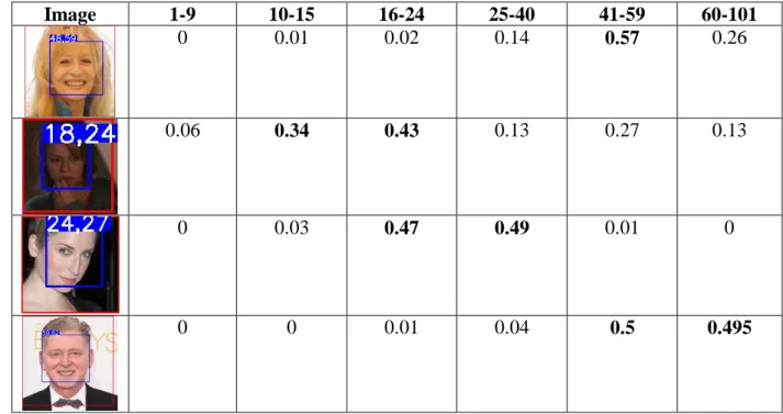
The network probabilities are initially computed for each of the 101 possible ages, i.e., considering 101 age classes. To compute the probabilities for the five group classes, the age-wise probabilities were grouped into age-group classes. So, in order to obtain the probability of agent-group class 1-9, we sum up all single probabilities from age class 1 to age class 9. Our tests showed that for some cases, usually the ones that lie near the edge of another class, the softmax classifier has a distribution similar between the two adjacent classes. As an example, we can analyze row 3 and row 4 from Table 4. The person represented in row 3 has an actual age of 27 and the probability around classes 16-24 and 25-40 present similar values (i.e., 47% against 49%, respectively). The same applies to row 4, which represents a person whose actual age is 62 years,

(43)

28 resulting in a similar probability for classes 41-59 and 60-101 (i.e., 50% and 49.5%, respectively). In these specific cases, it is clearly difficult to predict to which of the classes the person actually belongs. Ideally, data samples would produce results similar to the ones obtained for the one represented in the first row, for which the prediction points to class 41-59 with a confidence value significantly higher than the ones obtained for the alternative age-group classes. This case has strong confidence in the predicted class and is, in fact, correct since the person has a real age of 59 years.

Table 4- Samples with the softmax probability distribution by class.

Image 1-9 10-15 16-24 25-40 41-59 60-101

0 0.01 0.02 0.14 0.57 0.26

0.06 0.34 0.43 0.13 0.27 0.13

0 0.03 0.47 0.49 0.01 0

0 0 0.01 0.04 0.5 0.495

But before doing any conclusions, let us analyze the whole validation data and see how the accuracy performs on all the samples, and let us see if in fact cases where the probability is higher, are most of the times correct or not.

Table 5- Accuracy using different probability ranges (p stands for probability).

Success Fail

Age ( p <60%) 1180 (39%) 1822 (61%) Age ( p >=60%) 2562 (71%) 1042 (29%) Gender (0.25 < p < 0.75) 227 (63%) 133(37%) Gender (p <= 0.25 OR p >= 0.75) 5987 (96%) 259 (4%)

(44)

29 From the results present in Table 5, we can see that there are a lot of examples that fail with a probability lower than 60% on the predicted class. But on the other hand, when probabilities are higher than 60%, we can also verify a lot of failed examples (1042). These numbers seem to be considerably high in order to proceed with a manual validation on them all - validating manually more than 1000 examples is very time-consuming. There are also several correct examples that are predicted with less than 60% probability. On top of that, even validating ages manually is not completely accurate – even for humans, some cases might be hard to predict due to diverse conditions, as light, makeup, and angles. Therefore, there is a need to find an additional automatic mechanism to increase the confidence with which these examples are classified.

When it comes to gender classification, we have a higher overall accuracy on the tested network. Also, manual validation is simpler for humans since there are only two classes available (i.e., man and woman). For gender, the prediction is made differently from the one for age classification. The output of the model is a value that ranges from 0 to 1, where values greater than 0.5 are considered as a male classification, and values smaller than 0.5 are classified as a woman. So the network does provide a single probability as output, rather than multiple ones. If we consider probabilities near 0.5 as low confident, we may expect that most misclassified samples to be classified with probabilities near that reference value. Tests were done based on this assumption by checking how many samples are misclassified with a probability between 0.25 and 0.75, how many with a probability below 0.25 and how many with a probability above 0.75. This is expected to give us the amount of misclassified samples for which the network is not confident with its prediction. Results for this are shown in Table 5.

The results show that the probability of the network failing the predictions is higher when the probability of the prediction has confidence near 0.5. Although we still have more failed examples on high confidence inputs, proportionally to the total samples, they represent a smaller proportion of images. The amount of failed examples are not extensive and, thus, manually validating them is easier than for the age case. We conclude that a manual validation approach when the probability of the prediction is near 0.5 is able to improve the statistics with an acceptable level of human intervention.

(45)

30 3.7. Increase the accuracy of low confidence outputs

Followed by previous analysis, the network would benefit from having another mechanism to increase the correctness of a prediction when our base model has a confidence smaller than 60%, when it comes to age classification, or confidence near the reference value of 0.5, for gender classification. Instead of applying a manual validation, ideally, we would have an automated mechanism for it.

Siamese networks using One-Shot Learning could be useful to compare a face against a database of pre-determined faces, and based on similarity levels, predict the person’s class. If we use children’s faces, it is more likely that it will be more similar to another child’s face than if we compare it against an adult. This is because there are facial landmarks that clearly differentiate a child from an adult. If this hypothesis is true, then there would be no need for a manual validation system because this mechanism could increase the accuracy of the network further.

To test this hypothesis, we used Openface’s framework [31], which has a comparison module based on Siamese Networks to compare people’s faces. For this, both faces pass through the same model, and this model outputs a squared L2 distance (Euclidean distance) between both images. This means that lower output scores represent more similarity between the inputs.

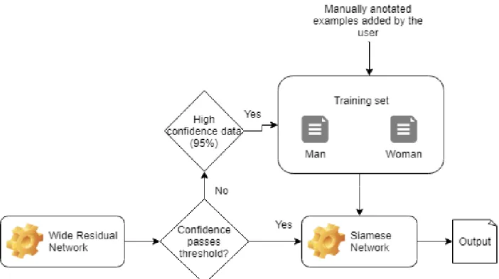
The faces used were the ones with lower confidence levels extracted from the dataset that was tested previously with the Wide Residual Network. The One-Shot training dataset was composed of pictures that were correctly predicted with greater confidence (95%) by the system because those showed to have a high classification rate and are therefore more trustworthy. In total, this was composed of a total of 3002 test examples and around 30 validation images for each of the used classes. Using a smaller training dataset allows the network to do computations faster since it is executed fewer times (once for each of the dataset images).

This can be viewed in Figure 8, where it is shown how the training data was created and how it feeds the Siamese Network. The training set represents a folder where it has 2 distinct additional folders, one where the images for men are stored, and another folder for women. Those pre-added images can also be removed, and the user can include new samples manually. Subsequentially, this training set is fed to the Siamese Network in order to compare them against the input that we want to validate, and an output prediction is the result of that computation.

(46)

31

Figure 8- One-Shot training data creation flow.

On a first experiment, the faces were compared against the validation dataset, and the prediction considered as correct was the one that was the most similar considering all the classes. So a man with 25 years would be compared against all faces from all classes, and if the most similar face would be from a face present in class 25-40, then that class would be the output prediction.

Table 6- Accuracy over ranking similarity for under-confident examples.

Success Fail

Age Minimum 1236 (41%) 1766 (59%) Age Average minimum 362 (12%) 2640 (88%)

Gender 271 (75%) 89 (25%)

This gave us the results present in Table 6, under the “Age minimum” test. The accuracy was similar to the one obtained using only the age classification model, so there was no improvement in including this additional network. Samples from such an experiment are shown in Figure 9 and Figure 10, where the first one shows correctly predicted data, and the second shows the failed examples. The first face in each case was the one that was tested. Therefore the second

(47)

32 image (on the right side) is the image from the validation data. The real classes for each image are described below itself.

Figure 9- Age correctly predicted data. Left side image is the input image, while the right side image is the validation image to which the input was matched.

Figure 10- Age failed prediction data. Left side image is the input image, while the right side image is the validation image to which the input was matched.