LI")
M
M
...
V"l
U
Z
- '
Beniamino Murgante Osvaldo Gervasi
Sanjay Misra Nadia Nedjah
Ana Maria A.C. Rocha David Taniar
Bernady O. Apduhan (Eds.)
Computational Science
and Its Applications
-ICCSA 2012
12th International Conference
Salvador do Bahia, Brazil, luno
2012
A Derivative-Free Filter Driven Multistart
Technique for Global Optimization
Florbela P. Fernandes1,3, M. Fernanda P. Costa2,3, and Edite M. G. P.
Fernandes4
1
Polytechnic Institute of Bragan¸ca, ESTiG, 5301-857 Bragan¸ca, Portugal,
2
Department of Mathematics and Applications, University of Minho, 4800-058 Guimar˜aes, Portugal,
3
Mathematics R&D Centre,
4
Algoritmi R&D Centre,
University of Minho, 4710-057 Braga, Portugal
Abstract. A stochastic global optimization method based on a multi-start strategy and a derivative-free filter local search for general con-strained optimization is presented and analyzed. In the local search pro-cedure, approximate descent directions for the constraint violation or the objective function are used to progress towards the optimal solution. The algorithm is able to locate all the local minima, and consequently, the global minimum of a multi-modal objective function. The performance of the multistart method is analyzed with a set of benchmark problems and a comparison is made with other methods.
Keywords: Global optimization, Multistart, Descent Direction, Filter Method
1
Introduction
Global optimization problems arise in many engineering applications. Owing to the existence of multiple minima, it is a challenging task to solve a multilocal optimization problem and to identify all the global minima.
The purpose of this paper is to present a technique for solving constrained global optimization problems based on a multistart method that uses a filter methodology to handle the constraints of the problem. The problem to be ad-dressed is of the following type
minf(x)
subject togj(x)≤0, j= 1, ..., m
li≤xi≤ui, i= 1, ..., n (1)
where, at least one of the functionsf, gj :Rn−→Ris nonlinear and F ={x∈
Problems with general nonlinear equality constraints can be reformulated in the above form by introducing h(x) = 0 as inequality constraints |h(x)| −τ ≤ 0, where τ is a small positive relaxation parameter. Since this kind of problems may have many global and local (non-global) optimal solutions (convexity is not assumed), it is important to develop a methodology that is able to explore the entire search space, find all the (local) minima guaranteeing, in some way, that convergence to a previously found minimum is avoided, and identify the global ones.
The two major classes of methods for solving problem (1) globally are the deterministic and the stochastic one. One of the most known stochastic algo-rithms is the multistart. In the last decade some research has been focused on this type of methods [1, 6, 9–11]; see also [7] and the references therein included. The underlying idea of this method is to sample uniformly a point from the search region and to perform a local search, starting from this point, to obtain an optimal (local) solution, using a local technique. This is repeated until the stop conditions are met. One of the advantages of multistart is that it has the potential of finding all local minima; although, it has the drawback of locating the same solution more than once.
Here, we are specially interested in developing a simple to implement and efficient method for the identification of at least one global optimal solution of problem (1) that is based on a multistart paradigm. A multistart strategy is chosen due to its simplicity and previously observed practical good performance. The herein proposed method does not compute or approximate any deriva-tives or penalty parameters. Our proposal for the local search relies on a pro-cedure, namely, the approximate descent direction (ADD) method, which is a derivative-free procedure with high ability of producing a descent direction. The ADD method is combined with a (line search) filter method to generate trial solutions that might be acceptable if they improve the constraint violation or the objective function. Hence, the progress towards a solution that is feasible and optimal is carried out by a filter method. This is a recent strategy that has shown to be highly competitive with penalty function methods [2–4].
This paper is organized as follows. In Section 2, the algorithm based on the multistart strategy and on the filter methodology is presented. In Section 3, we report the results of our numerical experiments with a set of benchmark problems. In the last section, conclusions are summarized and recommendations for future work are given.
2
The Filter Driven Multistart Method
that computes approximate descent directions, for either the constraint violation or the objective function, is implemented with reduced computational costs. To measure progress towards an optimal solution a filter methodology, as outlined in [4], is integrated into the local search procedure. The filter methodology ap-pears naturally from the observation that an optimal solution of the problem (1) minimizes both constraint violation and objective function [2, 3, 5, 4].
2.1 A Multistart Strategy
The basic multistart algorithm starts by randomly generating a point x from the search space S ⊂ Rn, and a local search procedure is applied from x to converge to a local minimumy. We will denote the implementation of the local procedure to provide the minimumy byy=L(x). Subsequently, another point is randomly generated from the search space and the local search is again applied to give another local minimum. This process is repeated until a stopping rule is satisfied. The pseudo-code of this procedure is presented below in Algorithm 1.
Algorithm 1Basic multistart algorithm
1: Setk= 1;
2: Randomly generatexfromS; 3: Computey1=L(x);
4: whilethe stopping rule is not satisfieddo 5: Randomly generatexfromS;
6: Computey=L(x);
7: if y /∈ {yi, i= 1, . . . , k}then
8: k=k+ 1; 9: Setyk=y;
10: end if 11: end while
Unfortunately, this multistart strategy has a drawback since the same local minimum may be found over and over again. To prevent the repetitive invo-king of the local search procedure, converging to previously found local minima, clustering techniques have been incorporated into the multistart strategy. To guarantee that a local minimum is found only once, the concept of region of attraction of a local minimum is introduced.
Definition 1. The region of attraction of a local minimum associated with a local search procedure Lis defined as:
Ai≡ {x∈ S, yi=L(x)}, (2)
This concept is very important because it guarantees that the local search applied to any pointxfrom the region of attractionAi will converge eventually
to the same minimizer yi. Thus, after yi has been found there is no point in
starting the local search from any other point in that region of attraction. LetN be the number of local minima inS. From the previous definition it follows that
S=
N
[
i=1
Ai andAi∩Aj=∅, fori6=j. (3)
A multistart method that uses the concept of region of attraction proceeds as follows: it starts by randomly generating a point from S, and applies a local search to obtain the first minimum y1 with the region of attraction A1.
After-wards, other points are randomly generated from S until a point is found that does not belong toA1. Next, the local search is performed and a new minimizer
y2 is obtained, with the region of attraction A2. The next point from which a
local search will start does not belong toA1∪A2. This procedure continues until
a stopping rule is satisfied. The corresponding multistart algorithm is presented in the Algorithm 2:
Algorithm 2Multistart Clustering algorithm
1: Setk= 1;
2: Randomly generatexfromS;
3: Computey1=L(x) and the correspondingA1;
4: whilethe stopping rule is not satisfieddo 5: Randomly generatexfromS;
6: if x /∈ ∪k
i=1Aithen
7: Computey=L(x); 8: k=k+ 1;
9: Setyk=yand compute the correspondingAk;
10: end if 11: end while
Theoretically, this algorithm invokes the local search procedure onlyN times, where N is the number of existing minima of (1). In practice, the regions of attraction Ak of the minima found so far are not easy to compute. A simple
stochastic procedure is used to estimate the probability, p, that a randomly generated point will not belong to a specific set, which is the union of a certain number of regions of attraction, i.e.,p=P[x /∈ ∪k
i=1Ai]. Using this reasoning, the
new steps of the regions of attraction based multistart algorithm are described in Algorithm 3.
The probabilitypis estimated as follows [11]. Let the maximum attractive radius of the minimizeryi be defined by:
Ri= max j
n x
(j)
i −yi
o
Algorithm 3Ideal Multistart algorithm
1: Setk= 1;
2: Randomly generatexfromS;
3: Computey1=L(x) and the correspondingA1;
4: whilethe stopping rule is not satisfieddo 5: Randomly generatexfromS;
6: Computep=P[x /∈ ∪k i=1Ai];
7: Letζ be a uniform distributed number in (0,1); 8: if ζ < pthen
9: Computey=L(x);
10: if y /∈ {yi, i= 1, ..., k}then
11: k=k+ 1;
12: Setyk=yand compute the correspondingAk;
13: end if 14: end if 15: end while
where x(ij) are the generated points which led to the minimizer yi. Given a
randomly generated point x, let z = kx−yik
Ri . Clearly, if z ≤ 1 then xis likely
to be inside the region of attraction of yi. On the other hand, if the direction
from xto yi is ascent then xis likely to be outside the region of attraction of
yi. Based on a suggestion presented in [11], an estimate of the probability that
x /∈Ai is herein computed by:
p(x /∈Ai) =
1, if z >1 or the direction from x to yi is ascent
̺ φ(z, l), otherwise (5)
where 0 ≤ ̺ ≤ 1 is a factor that depends on the directional derivative of f
along the direction from x to yi, l is the number of times yi has been
identi-fied/recovered so far and the functionφ(z, l) satisfies the properties:
lim
z→0φ(z, l)→0, zlim→1φ(z, l)→1, llim→∞φ(z, l)→0 and 0< φ(z, l)<1.
In the Ideal Multistart method [11], Voglis and Lagaris propose the
φ(z, l) =zexp −l2(z−1)2
for all z∈(0,1). (6)
Since the Algorithm 3 has the potential of finding all local minima and one global solution is to be required, each solution is compared with the previously identified solutions and the one with the most extreme value is always saved.
2.2 The Derivative-Free Filter Local Procedure
Direction Filter (ADDF) method. The pointyis computed based on a direction
dand a step sizeα∈(0,1] in such a way that
y=x+α d. (7)
The procedure that decides which step size is accepted to generate an accept-able approximate minimizer is a filter method. The herein proposed multistart method uses the filter set concept [4] that has the ability to explore both feasible and infeasible regions. This technique incorporates the concept of nondominance, present in the field of multiobjective optimization, to build a filter that is able to accept a trial point if it improves either the objective function or the con-straint violation, relative to the current point. Filter-based algorithms treat the optimization problem as a biobjective problem aiming to minimize both the ob-jective function and the nonnegative constraint violation function. In this way, the previous constrained problem (1) is reformulated as a biobjective problem involving the original objective functionf and the constraint violation function
θ, as follows:
min
x∈S(f(x), θ(x)) (8)
where forβ ∈ {1,2}
θ(x) =
m
X
i=1
max
i {0, gi(x)}
β +
n
X
i=1
max
i {0, xi−ui}
β
+max
i {0, li−xi}
β
.
(9) After a search direction d has been computed, a step size α is determined by a backtracking line search technique. A decreasing sequence ofαvalues is tried until a set of acceptance conditions are satisfied. The trial point y, in (7), is acceptable if sufficient progress in θ or in f is verified, relative to the current pointx, as shown:
θ(y)≤(1−γθ)θ(x) or f(y)≤f(x)−γfθ(x) (10)
whereγθ, γf ∈(0,1). However, whenxis (almost) feasible, i.e., in practice when
θ(x)≤θmin, the trial point yhas to satisfy only the condition
f(y)≤f(x)−γfθ(x) (11)
to be acceptable, where 0< θmin≪1. To prevent cycling between points that
improve either θ or f, at each iteration, the algorithm maintains the filter F which is a set of pairs (θ, f) that are prohibited for a successful trial point. During the backtracking line search procedure, they is acceptable only if (θ(y), f(y))∈/ F. If the stopping conditions are not satisfied (see (14) ahead), x←y and this procedure is repeated.
The filter is initialized with pairs (θ, f) that satisfyθ≥θmax, whereθmax>0
is the upper bound onθ. Furthermore, wheneveryis accepted because condition (10) is satisfied, the filter is updated by the formula
F=F ∪
When it is not possible to find a point y with a step size α > αmin (0 <
αmin<<1) that satisfy one of the conditions (10) or (11), a restoration phase is
invoked. In this phase, the algorithm recovers the best point in the filter, herein denoted by xbest
F , and a new trial point is determined according to the strategy
based on equation (7).
The algorithm implements the ADD method [5] to compute the directiond, required in (7). This strategy has a high ability of producing a descent direction for a specific function. The ADD method is a derivative-free procedure which uses several points around a given point x ∈ Rn to generate an approximate descent direction for a function ψat x[5]. More specifically, the ADD method choosesrexploring points close tox, in order to generate an approximate descent directiond∈Rnforψatx. Hence, the directiond= v
kvk is computed atx, after
generatingrpoints{ai}ri=1 close tox, as shown:
v=
r
X
i=1
wiei (12)
where
wi=
∆ψi r
X
j=1
|∆ψj|
, ∆ψi=ψ(ai)−ψ(x), i= 1, . . . , r
ei =−
ai−x
kai−xk
i= 1, . . . , r.
(13)
In the ADDF context, the ADD method generates the search direction d, at a given pointx, according to the following rules:
– Ifx is feasible (in practice, if θ(x) < θtol), the ADD method computes an
approximate descent directiondfor the objective function f atxand then
ψ=f in (13);
– Ifxis infeasible, the ADD method is used to compute an approximate de-scent directiond for the constraint violation function θ, at x, and in this caseψ=θ.
To judge the success of the ADDF algorithm, the three below presented conditions are applied simultaneously, i.e., if
|f(y)−f(x)| ≤10−4|f(y)|+ 10−6 ∧ |θ(y)−θ(x)| ≤10−4θ(y) + 10−6
∧ ky−xk ≤10−4
kyk+ 10−6 (14)
Algorithm 4ADDF algorithm
Require: x(sampled in multistart); Setxbest
F =xand ˜x=x;
1: Initialize the filter;
2: whilethe stopping conditions are not satisfieddo 3: Setx= ˜x;
4: Use ADD to computevby (12); 5: Setα= 1;
6: Computeyusing (7);
7: whilenew trialyis not acceptabledo
8: Check acceptability of trial point, using (10) and (11); 9: if acceptable by the filterthen
10: Update the filter if appropriate; 11: Set ˜x=y; Updatexbest
F ;
12: else
13: Setα=α/2;
14: if α < αmin then
15: Setα= 1; Setx=xbest F ;
16: Invoke restoration phase; 17: end if
18: Computeyusing (7);
19: end if 20: end while 21: end while
2.3 Stopping Rule
Good stopping rules to identify multiple optimal solutions should combine re-liability and economy. A reliable rule is one that stops only when all minima have been identified with certainty. An economical rule is one that invokes the local search the least number of times to verify that all minima have been found. A lot of research about stopping rules has been carried out in the past (see [6] and the references therein included). There are three established rules that have been successfully used [6].
We choose to use the following stopping condition [6]. Ifsdenotes de number of recovered local minima after having performedtlocal search procedures, then the estimate of the fraction of the uncovered space is given by
P(s) = s(s+ 1)
t(t−1) (15)
and the stopping rule is
P(s)≤ǫ (16)
3
Experimental Results
The MADDF method was coded in MatLab and the results were obtained in a PC with an Intel(R) Core(TM)2 Duo CPU P7370 2.00GHz processor and 3 GB of memory.
To perform some comparisons between other methods, it is necessary to set the MADDF parameters. The parameter τ used to reformulate equality into inequality constraints was set toτ= 10−5. Since derivatives are not provided to
the algorithm, the factor̺is estimated and set to 0.05. The closer the direction (y −x) is to the greatest decrease of f, the smaller is ̺. The power factor used in equation (9) was set to 2 and to generate the approximate descent directions we set r = 2 and rADD = 10−3 (the radius of the neighborhood in
which the exploring points are generated), as suggested in [5]. In ADDF method,
γθ=γf = 10−5,αmin= 10−6,θtol = 10−5,θmin= 10−3max{1,1.25θ(xinitial)},
θmax = max{1,1.25θ(xinitial)}, where xinitial is the initial point in the local
search.
In this section, we report the performance of the MADDF algorithm on 14 well-known test problems, which are shown in the Appendix of this paper, in an effort to make the article as self-contained as possible. The MADDF code was applied 30 times to solve each problem.
In the first set of experiments, summarized in Table 1, the stopping rule (16) withǫ= 0.06 is used. Table 1 summarizes the MADDF results obtained for each
Table 1.Numerical results obtained with MADDF and FSA [5].
Prob. fOP T Method Best Average Worst S.D. Av. f.eval.
g3 -1 MADDF -1.0000968 -0.9998019 -0.9993183 0.000208 45466
in [5] -1.0000015 -0.9991874 -0.9915186 0.001653 314938 g6 -6961.81388 MADDF -6961.23915 -6957.99845 -6954.65040 1.92544 15544 in [5] -6961.81388 -6961.81388 -6961.81388 0.00000 44538 g8 -0.095825 MADDF -0.095825 -0.095825 -0.095825 0.000000 4999 in [5] -0.095825 -0.095825 -0.095825 0.000000 56476 g9 680.630057 MADDF 681.08698 683.31319 685.49488 1.38392 38099 in [5] 680.63008 680.63642 680.69832 0.014517 324596
g11 0.75 MADDF 0.749980 0.750204 0.751048 0.000295 139622
in [5] 0.749999 0.749999 0.749999 0.000000 23722
test problem as well as the best known objective function value for each problem (‘fOP T’). In order to show more details concerning the quality of the obtained
Problems g3 and g8 were originally maximization problems. They were rewrit-ten as minimization problems. As it can be seen, for all five problems, MADDF method finds the global minimum. The quality of the solution is good. The worst results are obtained with problems g6 and g9. The average number of function evaluations is much smaller than the one reported by FSA method, for all test problems, except g11. In [5], a comparison with four evolutionary algorithms (EA) was made. These EA methods need a higher number of function evalua-tions than FSA and, consequently, our proposed method. Hence, the MADDF is better than the EA methods used in [5] as far as the number of function evaluations is concerned. These four EA-based methods are: Homomorphous Mappings (HM) method, Stochastic Ranking (SR) method, Adaptive Segrega-tional Constraint Handling EA (ASCHEA) method and Simple Multimembered Evolution Strategy (SMES) method. In Table 2, the results of the proposed MADDF method are repeated, in order to compare them with those of the EA methods. We may observe that the MADDF method is competitive with the EA methods relative to the quality of the solution.
Table 2.Numerical results obtained with MADDF and EA methods [5].
Prob. Method Best Average Worst
g3 MADDF -1.0000968 -0.9998019 -0.9993183
HM -0.9997 -0.9989 -0.9978
SR -1.000 -1.000 -1.000
ASCHEA -1 -0.99989 N.A
SMES -1.001038 -1.000989 -1.000579
g6 MADDF -6961.23915 -6957.99845 -6954.65040
HM -6952.1 -6342.6 -5473.9
SR -6961.814 -6875.940 -6350.262
ASCHEA -6961.81 -6961.81 N.A
SMES -6961.813965 -6961.283984 -6961.481934
g8 MADDF -0.095825 -0.095825 -0.095825
HM -0.0958250 -0.0891568 -0.0291438
SR -0.095825 -0.095825 -0.095825
ASCHEA -0.09582 -0.09582 N.A
SMES -0.095826 -0.095826 -0.095826
g9 MADDF 681.08698 683.31319 685.49488
HM 680.91 681.16 683.18
SR 680.630 680.656 680.763
ASCHEA 680.630 680.641 N.A
SMES 680.631592 680.643410 680.719299
g11 MADDF 0.749980 0.750204 0.751048
HM 0.75 0.75 0.75
SR 0.750 0.750 0.750
ASCHEA 0.75 0.75 N.A
To establish other comparisons with other stochastic global methods, we ap-plied the following conditions that appear in [8] to the next set of nine problems and the results are shown in the next two tables. Two conditions to judge the success of the run were applied. First,
f(xbest)−fOP T
≤10−4|fOP T| (17) wheref(xbest) is the best solution found so far and f
OP T is the known optimal
solution available in the literature, is used instead of the stopping rule (16). In practice, when solving any benchmark problem whose global optimal so-lution is known, the Algorithm 3 is stopped as soon as a sufficiently accurate solution is found, according to the condition in (17). We remark that in mul-tistart clustering methods based on the region of attraction, the stopping rule of the algorithm is crucial to promote convergence to all local optimal solutions (cf. [6]). In the presented algorithm, the likelihood of choosing a point that does not belong to the regions of attraction of previously identified optimal solutions is very high, although convergence to a local minimum that has not been located before is not guaranteed. Convergence to an optimal solution more than once may happen. So far, during the herein presented experiments this situation has occurred although not frequently.
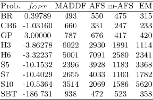
Table 3 contains the average number of function evaluation obtained after the 30 runs. A comparison is made with the results reported in [8] - two artifi-cial fish swarm based methods (AFS and m-AFS) and an electromagnetism-like mechanism algorithm (EM).
Table 3.Average number of function evaluations, using (17).
Prob. fOP T MADDF AFS m-AFS EM
BR 0.39789 493 550 475 315
CB6 -1.03160 660 331 247 233
GP 3.00000 787 676 417 420
H3 -3.86278 6022 2930 1891 1114 H6 -3.32237 5001 7091 2580 2341 S5 -10.1532 2396 3928 1183 3368 S7 -10.4029 2655 4033 1103 1782 S10 -10.5364 3514 2069 1586 5620
SBT -186.731 938 472 523 358
From the table we may conclude that the performance of the proposed MADDF is similar to the AFS algorithm, in terms of efficiency (number of function evaluations), while m-AFS and EM are slightly better than MADDF.
The results shown in Table 4 were obtained using the following stopping condition,
f(xbest)−fOP T
instead of (16). This set of experiments is compared with the results obtained by AFS, m-AFS, two particle swarm algorithms, PSO-RPB and PSO-HS, and a differential evolution method, DE, available in [8].
Table 4.Average number of function evaluations, using (18).
Prob. fOP T MADDF AFS m-AFS PSO-RPB PSO-HS DE
BR 0.39789 506 651 438 2652 2018 1305
CB6 -1.03160 660 246 245 2561 2390 1127
GP 3.00000 1063 562 485 2817 1698 884
H3 -3.86278 5845 1573 1142 3564 2948 1238
H6 -3.32237 7559 7861 2845 8420 8675 7053
S5 -10.1532 2929 3773 1150 6641 6030 5824
S7 -10.4029 4428 2761 1240 6860 6078 5346
S10 -10.5364 4489 2721 1190 6747 5602 4822
SBT -186.731 1867 659 516 4206 6216 2430
As it can be seen, the MADDF method has a similar performance to AFS method, outperforms the two variants of the particle swarm optimization and the differential evolution methods, although is less efficient than m-AFS.
4
Conclusions and Future Work
We present a multistart technique based on a derivative-free filter method to solve constrained global optimization problems. The multistart strategy relies on the concept of region of attraction to prevent the repetitive use of the local search procedure in order to avoid convergence to previously found local minima. Our proposal for the local search computes approximate descent directions combined with a (line search) filter method to generate a sequence of approximate solutions that improve either the constraint violation or the objective function value.
A set of 14 well-known test problems was used and the results obtained are very promising. In all problems we could reach the global minimum and the performance of the algorithm, in terms of number of function evaluations and the quality of the solution is quite satisfactory.
In the future, we aim to extend MADDF method to multilocal programming, so that all global as well as local (non-global) minimizers are obtained. This is an interesting and promising area of research due to their real applications in the chemical engineering field.
Acknowledgments. The authors wish to thank three anonymous referees for their valuable comments and suggestions to improve the paper.
References
1. Ali, M.M., Gabere, M.N.: A simulated annealing driven multi-start algorithm for bound constrained global optimization. Journal of Computational and Applied Mathematics. 233, 2661-2674 (2010)
2. Audet, C., Dennis, Jr., J.E.: A pattern search filter method for nonlinear program-ming without derivatives. SIAM Journal on Optimization. 14(4) 980–1010 (2004) 3. Costa, M.F.P., Fernandes, E.M.G.P.: Assessing the potential of interior point barrier
filter line search methods: nonmonotone versus monotone approach. Optimization. 60(10-11), 1251–1268 (2011)
4. Fletcher, R., Leyffer, S.: Nonlinear programming without a penalty function. Math-ematical Programming. 91, 239–269 (2002)
5. Hedar, A.R., Fukushima, M.: Derivative-Free Filter Simulated Annealing Method for Constrained Continuous Global Optimization. Journal of Global Optimization. 35, 521–549 (2006)
6. Lagaris, I.E., Tsoulos, I.G.: Stopping rules for box-constrained stochastic global optimization. Applied Mathematics and Computation. 197, 622–632 (2008) 7. Marti, R.: Multi-start methods. In: Glover F, Kochenberger G (eds) Handbook of
metaheuristics. pp 355–368. Kluwer, Dordrech (2003)
8. Rocha, A.M.A.C., Fernandes, E.M.G.P.: Mutation-Based Artificial Fish Swarm Al-gorithm for Bound Constrained Global Optimization. In: Numerical Analysis and Applied Mathematics ICNAAM 2011 AIP Conf. Proc. 1389, 751–754 (2011) 9. Tsoulos, I.G., Lagaris, I.E.: MinFinder: Locating all the local minima of a function,
Computer Physics Communications. 174, 166–179 (2006)
10. Tu, W., Mayne, R.W.: Studies of multi-start clustering for global optimization. In-ternational Journal for Numerical Methods in Engineering. 53(9), 2239–2252 (2002) 11. Voglis, C., Lagaris, I.E.: Towards ”Ideal Multistart”. A stochastic approach for locating the minima of a continuous function inside a bounded domain. Applied Mathematics and Computation. 213, 1404–1415 (2009)
Appendix - Test problems
– Branin (BR)
minf(x)≡(x2−45π.12x
2
1+π5x1−6)
2+ 10 1
− 1
8π
cos(x1) + 10
subject to −5≤x1≤10
0≤x2≤15
– Camel (CB6)
minf(x)≡4−2.1x2 1+x
4 1
3
x2
1+x1x2−4(1−x22)x22
subject to −2≤xi ≤2, i= 1,2
– Goldestein and Price (GP)
minf(x)≡(1 + (x1+x2+ 1)2(19−14x1+ 3x21−14x2+ 6x1x2+ 3x22))×
×(30 + (2x1−3x2)2(18−32x1+ 12x21+ 48x2−36x1x2+ 27x22))
– Hartman3 (H3)
minf(x)≡ −
4
X
i=1
ciexp
−
3
X
j=1
aij(xj−pij)2
subject to 0≤xi≤1, i= 1,2,3
with
a=
3 10 30 0.1 10 35 3 10 30 0.1 10 35 , c=
1 1.2
3 3.2
and p=
0.3689 0.117 0.2673 0.4699 0.4387 0.747 0.1091 0.8732 0.5547 0.03815 0.5743 0.8828
– Hartman6 (H6)
minf(x)≡ −
4
X
i=1
ciexp
−
6
X
j=1
aij(xj−pij)2
subject to 0≤xi≤1, i= 1, . . . ,6
witha=
10 3 17 3.5 1.7 8 0.05 10 17 0.1 8 14
3 3.5 1.7 10 17 8 17 8 0.05 10 0.1 14
, c= 1 1.2
3 3.2
and p=
0.1312 0.1696 0.5569 0.0124 0.8283 0.5886 0.2329 0.4135 0.8307 0.3736 0.1004 0.9991 0.2348 0.1451 0.3522 0.2883 0.3047 0.6650 0.4047 0.8828 0.8732 0.5743 0.1091 0.0381
– Shekel-5 (S5)
minf(x)≡ −
5
X
i=1
1
(x−ai)(x−ai)T +ci
subject to 0≤xi≤10, i= 1, . . . ,4
with a=
4 4 4 4 1 1 1 1 8 8 8 8 6 6 6 6 3 7 3 7
and c=
0.1 0.2 0.2 0.4 0.4
– Shekel-7 (S7)
minf(x)≡ −
7
X
i=1
1
(x−ai)(x−ai)T +ci
subject to 0≤xi≤10, i= 1, . . . ,4
a=
4 4 4 4 1 1 1 1 8 8 8 8 6 6 6 6 3 7 3 7 2 9 2 9 5 3 5 3
and c=
0.1 0.2 0.2 0.4 0.4 0.6 0.3
– Shekel-10 (S10)
minf(x)≡ −
10
X
i=1
1
(x−ai)(x−ai)T +ci
subject to 0≤xi≤10, i= 1, . . . ,4
with a=
4 4 4 4 1 1 1 1 8 8 8 8 6 6 6 6 3 7 3 7 2 9 2 9 5 5 3 3 8 1 8 1 6 2 6 2 7 3.6 7 3.6
and c=
0.1 0.2 0.2 0.4 0.4 0.6 0.3 0.7 0.5 0.5
– Shubert (SBT)
minf(x)≡
5
X
i=1
icos((i+ 1)x1+i)
! 5 X
i=1
icos((i+ 1)x2+i)
!
subject to −10≤xi≤10, i= 1,2
– Problem G3
minf(x)≡ −(√n)nQn
i=1xi
subject to Pn
i=1x2i −1 = 0
0≤xi≤1, i= 1,2
– Problem G6
minf(x)≡(x1−10)3+ (x2−20)3
subject to −(x1−5)2−(x2−5)2+ 100≤0
(x1−6)2+ (x2−5)2−82.81≤0
13≤x1≤100
– Problem G8 minf(x)≡ −sin
3
(2πx1) sin(2πx2)
x3 1(x1+x2)
subject to x2
1−x2+ 1≤0
1−x1+ (x2−4)2≤0
0≤xi≤10, i= 1,2
– Problem G9
minf(x)≡(x1−10)2+ 5(x2−12)2+x43+ 3(x4−11)2+...
+10x6
5+ 7x26+x47−4x6x7−10x6−8x7
subject to v1 + 3v22+x
3+ 4x24+ 5x5−127≤0
7x1+ 3x2+ 10x23+x4−x5−282≤0
23x1+v2 + 6x62−8x7−196≤0
2v1 +v2−3x1x2+ 2x23+ 5x6−11x7≤0
−10≤xi≤10, i= 1, . . . ,7
withv1 = 2x2
1;v2 =x22
– Problem G11 minf(x)≡ −x2
1+ (x2−1)2
subject to x2−x21−1 = 0
![Table 1. Numerical results obtained with MADDF and FSA [5].](https://thumb-eu.123doks.com/thumbv2/123dok_br/16978514.762714/10.892.201.718.632.818/table-numerical-results-obtained-maddf-fsa.webp)
![Table 2. Numerical results obtained with MADDF and EA methods [5].](https://thumb-eu.123doks.com/thumbv2/123dok_br/16978514.762714/11.892.288.634.561.997/table-numerical-results-obtained-maddf-ea-methods.webp)