Cointegration and Structural Breaks in the EU
Sovereign Debt Crisis
Nuno Ferreira#1, Rui Menezes#2, Sónia Bentes*3
#Department of Quantitative Methods, IBS-ISCTE Business School, ISCTE Avenida das Forças Armadas, Lisboa, Portugal
1
2
*ISCAL
Avenida Miguel Bombarda, 20, Lisboa, Portugal 3
Abstract - First signs of a sovereign debt crisis spread
among financial players in the late 2009 as a result of the growing private and government debt levels worldwide. Late 2010, Trichet (then President of the ECB) stated that the sovereign debt crisis in Europe had become systemic. In an established crisis context, it was searched for evidence of structural breaks and cointegration between interest rates and stock market prices. A 13 year time-window was used in six European markets under stress. The results identified significant structural breaks at the end of 2010 and consistently rejected the null hypothesis of no cointegration.
.
Keywords ‐ Stock Markets Indices; Interest Rates; Structural Breaks; Cointegration; EU Sovereign Debt Crisis
1.
Introduction
The strategic positioning of European economies, namely interest rate fluctuations, stock market crises, regional effects of oil prices, regional political developments etc, makes them vulnerable to real and external shocks. In this context, Kurov [18] found that the monetary policy actions in bear market periods that have a strong effect on stocks can be revealing of greater sensitivity to changes in investor sentiment and credit market conditions. Overall, the results showed that the investor sentiment plays a significant role in monetary policy's effect on the stock market. Previous studies (e.g. Baker et al. [7]; Kumar and Lee [17] revealed that the investor sentiment predicts cross-section and aggregate stock returns indicating that it moves stock prices and, therefore, affects expected returns. This raises the question of whether the effect of monetary news on stocks is at least partially driven by the influence of FED or ECB policy on investor sentiment.
As a result of the financial crisis, modeling the dynamics of financial markets is gaining more popularity than ever among researchers for both academic and technical reasons. Private and public economic agents take a close interest in the movements of stock market indexes, interest rates, and exchange rates in order to make investment and economic policy decisions.
The most broadly used unit root test used to identify stationarity of the time series studied in the applied econometric literature is the Augmented Dickey Fuller test (henceforth ADF). However, several authors have stated that numerous price time series exhibit a structural change from their usual trend mostly due to significant policy changes. These economic events are caused by economic crises (e.g. changes in institutional arrangements, wars, financial crises, etc.) and have a marked impact on forecasting or analyzing the effect of policy changes in models with constant coefficients. As a result, there was strong evidence that the ADF test is biased towards null of random walk where there is a structural break in a time series. Such finding triggered the publication of numerous papers attempting to estimate structural breaks motivated by the fact that any random shock has a permanent effect on the system.
In the current context of crisis, this study analyzes structural break unit root tests in a 13 year time-window (1999-2011) for six European markets under stress, using the United States of America (US), the United Kingdom (UK) and Germany (GE) as benchmark. Considering the problems generated by structural breaks, two unit root tests were employed to allow for shifts in the relationship between unconditional mean of the stock markets and interest rate, namely: Zivot and Andrews [36] (henceforth ZA) and Lumsdaine and Papel [25] (henceforth LP). The ZA unit root test captures only the most significant structural break in each variable. A new approach to ____________________________________________________________________________________
International Journal of Latest Trends in Finance & Economic Sciences
IJLTFES, E‐ISSN: 2047‐0916
capture structural breaks was introduced by LP with the argument that a unit root test which identifies two structural breaks is much more robust. LP uses a modified version of the ADF test by incorporating two endogenous breaks. These two tests were chosen because they have three main advantages. Firstly, their properties are easily captured as they are ADF based tests. Secondly, the timing of the structural break is determined endogenously, and lastly, their computational implementation is easily accessible. To confirm the presence of structural breaks detected by ZA and LP tests, this paper also employs the method developed by Bai and Perron [3-6], (henceforth BP). This third test consistently estimates multiple structural changes in time series, their magnitude and the time of the breaks. However, it must be stressed that the consistency of the test depends on the assumption that time series are regime-wise stationary. This implies that breaks and break dates accurate with BP are only statistically reliable when the time series is stationary around a constant or a shifting level. If the time series is nonstationary, BP tests may detect that the time series has structural breaks.
A limitation of the ADF-type endogenous break unit root tests, e.g. ZA and LP tests, is that critical values are derived while assuming no break(s) under the null. Nunes et al. [30] and Lee and Strazicich [22-23] showed that this assumption leads to size distortions in the presence of a unit root with one or two breaks. As a result, one might conclude when using the ZA and LP tests that a time series is trend stationary, when, in fact, it is nonstationary with break(s), i.e. spurious rejections might occur. To address this issue, Lee and Strazicich [24] proposed a one-break Lagrange Multiplier (henceforth LM) unit root test as an alternative to the ZA test, while Lee and Strazicich [25] suggest a two-break LM unit root test as a substitute for the LP test. In contrast to the ADF test, the LM unit root test has the advantage that it is unaffected by breaks under the null. These authors proposed an endogenous LM type unit root test which accounts for a change in both the intercept and also in the intercept and slope. The break date is determined by obtaining the minimum LM t-statistic across all possible regressions. More recently, several studies started to apply the LM unit root test with one and two structural breaks to analyze the time series properties of macroeconomic variables (e.g. Chou [12]; Lean and Smyth [20-21].
Based on the studies cited above, we concluded the first part of the analysis assuming that the break
date is unknown and data-dependent. The distinct tests applied aimed to detect the most important structural breaks in the stock market and the interest rate relationship of all markets under analysis.
Having linked the source of the breaks found with some economic events during the time window under study, it was possible to advance with the second part of the analysis in which the main goal was to explore a possible cointegration relationship between interest rates and stock market prices. Therefore, the Gregory and Hansen [15] regime shift model (henceforth G-H) was used to find evidence of structural regime shifts that could explain the contamination of the severe EU debt crisis. The results identified the most significant structural breaks at the end of 2010 and consistently rejected the null hypothesis of no cointegration. Moreover, they showed that both the regional credit market and stock market have reached a nearly full integration in both pre and post crisis periods.
2.
Unit root tests and cointegration
under structural breaks
Structural changes or “breaks” appear to affect models based on key economic and financial time series such as output growth, inflation, exchange rates, interest rates and stock returns. This could reflect legislative, institutional or technological changes, shifts in economic policy, or even be due to large macroeconomic shocks such as the doubling or quadrupling oil prices of the past decades. A variety of classical and Bayesian approaches are available to select the appropriate number of breaks in regression models. Their diversity is essentially based on the type of break (e.g. breaks in mean; breaks in the variance; breaks in relationships; single breaks; multiple breaks; continuous breaks and some kind of mixed situations better described by smooth switching models).
The conventional stability and unit root tests are often associated with the concept of “persistence” of innovations or shocks to the economic system. In this context, the debate has been centered on whether shocks to macroeconomic time series have temporary or permanent effects. While Nelson and Plosser [29] suggested that most macroeconomic time series are best characterized by unit root processes implying that shocks to these series are permanent, Perron [32-33] challenged this by providing some evidence that the null hypothesis of a unit root test may be rejected for many macroeconomic time series if we allow for a
one-time shift in the trend function. Thus, it would be preferable to describe and characterize many macroeconomic time series as having temporary shocks (stationary) around a broken deterministic trend function. In essence, if there is a break in a deterministic trend, then the unit root tests (which implicitly assume the deterministic trend as correctly specified) will incorrectly conclude that there is a unit root, when, in fact, there is not. The policy effects can vary depending on both the nature of the non-stationarity associated with the macroeconomic variables, and the econometric modeling. Since the main focus of this paper is on the demand for money (interest rate) and stock markets, we could state that this relationship was subject to serious parameter instabilities (especially during periods of economic crises, institutional arrangements, wars, financial crises, etc.), which had a strong impact on capturing of policy changes effects. Many aggregated economic time series (consumption, income, interest rates, money, stock prices, etc.) display strong persistence with sizable fluctuations in both mean and variance over time. The classical approach to hypothesis testing is based on the assumption that the first two population moments (unconditional) are constant over time (covariance stationary) and hence unit roots pose a challenge for the usual econometric procedures.
Cointegration theory is very dependent on the existence of unit roots and is focused on the (long-run) equilibrium relationships. This relation, known as the cointegration relationship between the economic variables, shapes some economic equilibrium. It is well-known that some economic variables should not move freely or independently of each other; thus these connections persuade some econometricians to test for cointegration relationships within unit root tests by unconventional methods. Notwithstanding, an important limitation associated with the ADF test is the absence of any structural break effects. Dealing with finite samples, the standard tests for unit root (non-stationarity hypothesis test) are biased toward accepting the null hypothesis when the data-generating process is, in fact, stationary. Several other approaches to studying the estimated parameters stability are widely presented in the literature. Different theories on phases of economic development and growth postulate that an economic relationship changes over time. In the last three decades, the impact of structural changes on the result of econometric models has been of great concern. In this context, Perron [32] argued that if a structural break in a series is ignored, unit root tests
can be erroneous in rejecting the null hypothesis; on the other hand, if there is a break in the deterministic trend, unit root tests will mistakenly conclude that there is a unit root when, in fact, there is not. In short, an undetected structural break in a time series may lead to rejecting of the null hypothesis of unit roots.
Basically, there are two points of view on structural change modeling. The first assumes the structural change modeling as a known break point, and the other as unknown break points. Modeling structural changes by setting the break points in advance allows potential break-dates to be identified ex ante and the parameter constancy to be tested via the inclusion of interactive-dummy variables into the econometric models. In such cases, the hypothesis of a structural break can be tested by applying standard tests of significance with respect to estimated coefficients of these dummy variables. However this kind of test was subject to severe criticism due to the arbitrary nature of selected break-dates and the inability to identify when exactly the structural breaks had occurred. Therefore, another approach was proposed to model the structural breaks by assuming that the break date(s) are ex ante unknown. Each approach had several applications in the literature and presented different implications. A large number of papers derived asymptotic distributions for the null hypotheses of the structural change tests using different econometric approaches. The best known works in the enormous literature produced hitherto include Perron [32], Zivot and Andrews [36], Banerjee et al. [8] and Gregory and Hansen [15]. All these papers address unknown structural breaks procedures.
In this study, the authors carried out several tests with different variants in order to capture different structural breaks approaches in the relationship between stock market prices and interest rates. The estimation of the two breaks is performed simultaneously in both the time trend and the intercept. To this end, the following tests were performed and compared.
2. Data analysis
2.1. Zivot and Andrews test
The ZA is the most widely adopted endogenous one-break test. Building on Perron's exogenous break test, it only considers a break under the alternative but not under the null when carrying out unit root testing.
Of the three types of ADF test proposed by Perron, the authors applied the one in which the Ha is a break in the intercept and in the slope coefficient on the trend at an unknown breakpoint. Estimating by OLS:
1 1 2 2 1 1 yt t( ) t t( ) yt p i t i t (1) i D D y u
Thus many sequential regressions are computed where D1t (λ) and D2t (λ) change each time. The t-test statistic (concerning γ=0) is also computed in each regression. Zivot and Andrews [36] re-examined the Nelson-Plosser dataset and found a number of problems with the unit-root tests employed; thereafter, the literature documented an exhaustive list of empirical studies which employed this test (e.g. Ranganathan and Ananthakumar [34].
2.2. Lumsdaine and Papell test
Considering only one endogenous break may not be sufficient and lead to a loss of information, particularly when there is in fact more than one break. Lumsdaine and Papell [25] introduced a new approach to capture structural break with the argument that a unit root test that shows two structural breaks is much more robust. They contently reverse conclusions of many studies which fail to reject the null with the presence of one break. The LP test extends the tests for two structural breaks; models which consider two breaks in the intercept are known as AA, and those with two breaks in the intercept and slope of the trend are designated CC (also known as “crash-model”). The LP CC model can be specified as
0 1 1 1 1 2 2
:
(2)
:
t t t A t t t tH
x
c x
H
x
c
t d D
d
where D1t=1 for t > TB1 + 1 and 0 otherwise, D2t=1 for t > TB2 + 1 and 0 otherwise and TB1 and TB2 are the dates corresponding to the break points (mean shifts). The testing strategy employed in LP is similar to ZA, which implies following the ADF regression tests. The LP procedure generates a final t-statistic which is the greatest in absolute value (the most favorable for rejecting the null hypothesis). Consequently, the estimated breakpoints (TB1 and TB2) correspond to the minimum t-statistic.
The crucial effect of the trend property of the variables for the structural break estimation was
recognized by several authors. Ben-David and Papell [11] showed that the test power was affected by the inclusion of a trend variable where there is no upward trend in data. Otherwise it is inconvenient since the model may not capture some important patterns of the data without trend.
With this subjacent, Ben-David and Papell [10] and Ben-David et al. [9], used tests for a unit root against the alternative of broken trend-stationarity allowing for one and respectively two endogenous break points. This procedure, developed by Zivot and Andrews [36] and Lumsdaine and Papell [25], rejects the unit root null in favor of broken trend-stationarity for long-term US GDP. In all cases, the estimated breaks coincide with the Great Depression and/or World War II.
In accordance with this different conception of the distinct unit root tests allowing structural breaks, some more recent papers have combined several approaches to efficiently capture any sign of structural change (e.g. Marashdeh and Shrestha [27]; Ranganathan and Ananthakumar [37]).
2.3. Bai and Perron test
In The Bai and Perron [3-6] methodology to estimate and infer multiple mean breaks models based on dynamic linear regression models. They estimate the unknown break points given T observations by the least squares principle, and provide general consistency and asymptotic distribution results under fairly weak conditions, allowing for serial correlation and heteroskedasticity. In Bai et al. [2-3] the authors developed a sequential procedure to test the null hypothesis of one structural change versus the alternative of one plus one break in a single regression model. Thus, the pure structural change model is considered in several studies and is defined as j = 1, …,m + 1, t0=0 and tm+1 = T. The dependent variable is subject to m breaks and cj is the mean of the series, rt for each regime j. The model allows for general serial correlation and heterogeneity of the residuals across segments. The pure structural change model can be estimated as follows. For each m-partition, the least squares estimate of cj is obtained by minimizing the sum of squared residuals, where minimization occurs over all possible m-partitions.
Several authors have recently implemented the BP test for multiple break dates (e.g. Yu and Zivot [35]; Dey and Wang [13]).
2.4. Lee and Strazicich test
The first part of this empirical analysis ends with the LS test also known as LM test due to Langrage multipliers. The main advantage over previous tests is that they are not affected by structural breaks under the null hypothesis because the critical values of the ADF-type endogenous break unit root tests (such as ZA and LP) were derived while assuming no break(s) under the null. The test employed in this paper (model A, known as the “crash model”) could be briefly described considering:
Z
t
[1, ,
t D D
1t,
2t]
where DTjt =t-TBJ for t>=TBJ+1, j=1,2 and 0 otherwise. Consequently, it could be evidenced that DGP incorporated breaks under the null (β=1) and alternative hypothesis (β>1) as already noted. Making the value of β uncertain, we could rewrite the both hypotheses as: ,
: . (3)
Where v1t and v2t are stationary error terms. The LM unit root test statistic is obtained from one specific regression. Arghyrou [1] designed this component as the LM score principle. The LM test statistic is determined by testing the unit root null hypothesis that The LM unit root test determines the time location of the two endogenous breaks, whereas represent each combination of break points] using a grid search as follows: The break time should minimize this statistic. Critical values for a single break and two-break cases are tabulated from Lee and Strazicich [22-23] respectively. Another approach to searching for unit roots with breaks by allowing nonstationarity in the alternative hypothesis is adopted in several studies following the Lee and Strazicich procedure testing.
2.5. Gregory and Hansen test
Gregory and Hansen [15] used a residual-based test for cointegration in a multivariate time series with regime shifts; they proposed the ADF tests, which are
intended to test the null hypothesis of no cointegration against the alternative of cointegration in the presence of a possible regime shift. This test examines whether there has been a one-time shift in the cointegration relationship by detecting any cointegration in the possible presence of such breaks and presents four different approaches. A single-equation regression with structural change starting with the standard model of cointegration (model 1):
, 1, … , (4)
In this case, if there is stated a long-run relationship, µ and α are necessarily defined as time-invariant. The G-H approach consider that this long-run relationship could shift to a new long run relationship by introducing an unknown shifting point that is reflected in changes in the intercept µ and/or changes to the slope α defining Model 2 and 3 in the following form (model 2 - level shift (C)):
, 1, … , (5)
This model represents a level shift in the cointegration relationship, and is modeled as a change in the intercept µ variable µ1 and µ2 represent the intercept before and at the time of the shift. In order to account for the structural change, the authors introduced the dummy variable definition:
0 ,
1 . (6)
where the unknown parameter represents the relative timing of the change point and [.] denotes integer part. Model 3: Level Shift with Trend (C/T):
, 1, … , (7) In this model, the authors extended the possibilities by introducing a time trend βt into the level shift model. And finally, the model 4 - Regime Shift (C/S):
, 1, … , (8)
The last model integrates a shift in the slope vector, which permits the equilibrium relation to rotate and a parallel shift. For this case, α1 is the cointegrating slope coefficient before the regime shift, and α2 is the change in the slope coefficients, whereas
(
1
2)
is the cointegrating slope coefficient after the regime shift.
Concerning the software, all routines applied were run with WinRATS Pro 8.0 and are available in Estima website.
3. Dataset
The variables under study cover daily data from April 1999 to December 2012 and are expressed in levels after a logarithmization procedure. For instance, the stock market price (Pi), the (Y1) and (Y10) are the government bond yield and the interest rates at 1 year and 10 years, respectively. All the three variables have been collected for each selected market (Portugal (PT), Spain (SP), France (FR), Ireland (IR), Italy (IT) and Greece (GR)) from the European countries under most stress in the recent years. We also included the GE, UK and US markets as a benchmark. All data have been collected and are available online from Datastream database.
4. Results and Discussion
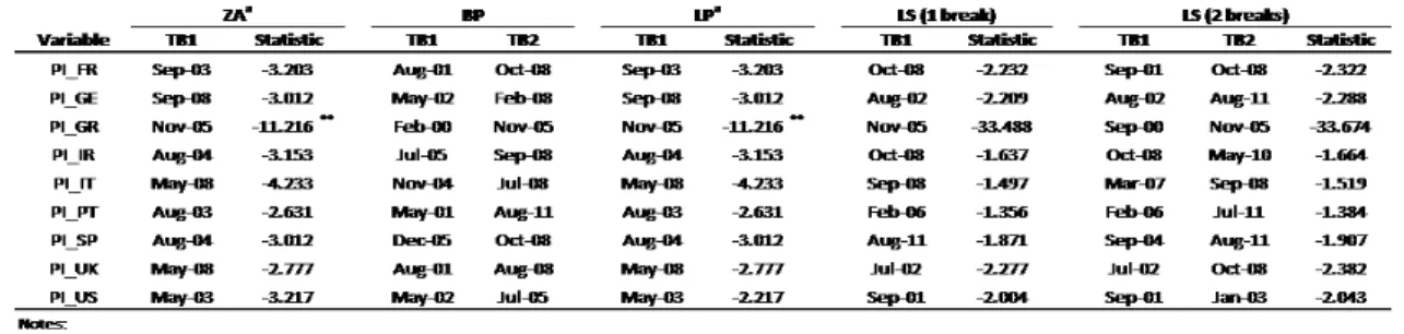
The authors ran a full battery of unit-root tests in line with similar studies (e.g. Pahlavani et al., [31]; Narayan and Smyth [28]; and more recently Maican et al. [26]. Thus, readers can make their own decision on mean reversion for a particular series, rather than only the best results with no mention of the number and specifications of tests tried. The results of the unit root testing procedures are presented in the tables below, starting with the price index (PI variable) (Table 1) which was implemented using both the intercept and trend options (ZA and LP tests). The corresponding time of the structural break (TB1 and TB2) for each variable is also shown in each test. For the PI variable in the established crisis period, the ZA and the LP tests fail to reject the null hypothesis of a unit-root at the 1 percent significance level in all countries except Greece. This means that the price index series of the remaining countries are non-stationary. For the 1 year interest rate (variable Y1) series (Table 2), both ZA and LP tests fail to reject the null hypothesis of a unit-root at 1 percent significance level in three countries – GE, US and UK.
Table 1 – Unit-root tests (variable PI). (**) indicates critical values at 1%. The optimal lag length was determined by SBC.
Table 2 - Unit-root tests (variable Y1(**) indicates critical values at 1%. The optimal lag length was determined by SBC.
Table 3 - Unit-root tests (variable Y10). (**) indicates critical values at 1%. The optimal lag length was determined by SBC.
The analyses of the 10 year interest rate (variable
Y10) series reveal that all countries are stationary (Table 3). In light of these results, the cointegration hypothesis was tested with the PI variable of all European countries (except GR) against the Y1 variable of GE (Table 4). The three most economically developed countries (GE, UK and US) revealed a similar pattern in the interest rate series, which could suggest a strong contagious phenomenon between them. The structural break points defined through the different tests consistently coincide with important dates through the time-window analyzed, with special emphasis on the US. According to Lee et al. [24] and citing Ghoshray and Johnson [14], by allowing for the possibility of a break in the null, the LM test can be considered genuine evidence of stationarity; this means that we can rely more on the break points calculated by the minimum LM test than those estimated by the remaining tests. This could lead to size distortion which increases with the magnitude of the break; this does not occur with the LM test as a different detrending method is used. Following these assumptions and focusing on the structural break points identified by the LM test (two breaks), all dates related to 2001-2003 reveal the economic impact of the September 11 attacks on the US, namely in New York City and Washington D.C. in 2001 and the repercussions in the following years with the concerted military action against Iraq.
Further, a mild recession in 2001, caused partly by the bursting of the dot-com bubble, prompted the Fed (led by Chairman Alan Greenspan) to lower the target federal funds rate from 6% to 1.75% in an effort to stimulate employment. The Fed kept interest rates low for the next two years; it dropped to just 1% - the lowest rate in 50 years - in summer 2003, and only rose again one year later. The Fed’s shift to this historically low interest rate coincided with the mid-2003 acceleration of housing prices. Although the outlook for the euro area's financial system has improved since late 2003, some potential sources of risk and
vulnerability remain. Within the financial system, pockets of fragility may still exist notably in the European banking sector. By late 2003, the US was in the midst of the most serious world economic setback, originated by the credit boom (interest rates were at a 50-year-low and mortgage credit stood at an all-time high) and the housing bubble (prices had exceeded all previous levels).
The first half of 2004 was characterized by a trend towards gradual economic recovery. However, there were still some obstacles hindering the growth of the world economy; for example, a rise in the price of oil per barrel to record high contributed to raise expectations in the major economic areas. In the US, 1.2 million new jobs were created, and core inflation rose from 1.1% to 1.9%, leading the Federal Reserve to raise interest rates by 25 basis points to 1.25 %. However, the European Central Bank kept the interest rate on the main refinancing operations at 2%. The Nasdaq rose 2.22% and the Dow Jones and S&P 500 showed variations of 0.18% and 2.60%. In the Eurozone, the Paris CAC 40 and IBEX 35 went up 4.92% and 4.41%, while the DAX in Frankfurt rose 2.64%.
During 2005, major equity markets continued their upward trend and the longer term interest rates declined.
As a result of concerns about the potential inflationary consequences of the ample liquidity supply and possible lagged effects of the sharp rise in energy prices on price and wage setting, the ECB raised interest rates by 25 basis points in early December 2005. The marked depreciation of the euro against the dollar from May 2005 could have also played a role. In the run-up to this decision, the ECB had considerably stepped up its use of moral suasion to signal its readiness to raise interest rates “at any time”. Despite this move, the monetary policy remained accommodated. This partly offset the easing of overall monetary conditions due to the weakening
of the euro; the ECB had taken this step in an attempt to bring short-term rates to a neutral position, as the United States Federal Reserve had done since July 2004.
Meanwhile, when the downturn in housing prices finally began in 2006, everyone had difficult in repaying their mortgages as home equity loans shrank. Subprime borrowers were, by definition, more prone to default on their mortgages than the average person. In addition, they were more likely to be poor and unemployed so had painfully few alternatives to defaulting. The resulting wave of subprime foreclosures fueled the aforementioned downward spiral of prices, as it prompted a glut in housing supply and a contraction of housing demand. The tendency of increasing prices (to enable increased subprime lending) was another dangerous feedback loop of the housing bubble. As housing prices rose, banks became more inclined to increase subprime lending, which in turn spurred greater housing demand, thereby accelerating the price increase. While such cycles seemed to enable the bubble to inflate itself, they still depended on adherence to the irrational belief that housing prices would rise indefinitely. Bankers who allowed rising prices to overshadow the risks of subprime lending did so in this belief. Mimicking and reinforcing homebuyers’ representativeness heuristic (i.e. the belief that recent trends would continue unabated), the behavior of such bankers further challenges the assumed rationality of key economic actors.
By 2007, more than just a few farsighted economists were noting that the unprecedented rise in housing prices might be an unsustainable bubble (though most still underestimated the bubble’s economic significance). Having plateaued in 2006, housing prices in 2007 stood on the edge of a precipice. They plummeted from the second quarter of that year until the first quarter of 2009, and fell 5% every three months i.e. faster than they had climbed. Housing prices continued to decline more gradually after 2009, sinking steadily through 2012 when they approached the pre-bubble, century-long average.
In 2008, developments took a turn for the worse, and the growth slowdown became acuter. In early 2009, the conclusion was that this would be a deeper recession than the average of “Big Five” (those in Spain, 1977; Norway, 1987; Finland, 1991; Sweden, 1991 and Japan, 1992). The conjuncture of elements is illustrative of the two channels of contagion:
cross-linkages and common shocks. There can be no doubt that the US financial crisis of 2007 spilled over into other markets through direct linkages. For example, German and Japanese financial institutions sought more attractive returns in the US subprime market. Due to the fact that profit opportunities in domestic real estate were limited at best and dismal at worst. Indeed, in hindsight, it became evident that many financial institutions outside the US had considerable exposure to the US subprime market. Similarly, the governments of emerging markets had experienced stress, although of mid-2009 sovereign credit spreads had narrowed substantially in the wake of massive support from rich countries for the IMF fund. European banks began to face liquidity problems after August 2007, and German banks continued to lend heavily to peripheral borrowers in the mistaken belief that peripheral countries were a safe outlet. Net exposure rose substantially in 2008. Speculators focused on Greek public debt on account of the country’s large and entrenched current account deficit as well as because of the small size of the market in Greek public bonds. Greece was potentially the start of speculative attacks on other peripheral countries – and even on countries beyond the Eurozone, such as the UK – that faced expanding public debt.
Greece thus found itself in a very difficult position in early 2010 and imposed cuts and raised taxes in order to pay high interest rates to buyers of its public debt. The country was able to access markets in January and March 2010, but the rate of interest was high on both occasions - well in excess of 6 percent. On 2 May 2010, the EU announced a support package for Greece, put together in conjunction with the IMF fund. Lapavitsas [19 ] documented that the sovereign debt crisis that broke out in Greece at the end of 2009 was fundamentally due to the precarious integration of peripheral countries in the Eurozone. Its immediate causes, however, lie with the crisis of 2007-9. The result in the Eurozone was a sovereign debt crisis, exacerbated by the structural weaknesses of monetary union. Meanwhile, with the global economy likely to perform indifferently in 2010-11 and given the high regional integration of European economies, exports were unlikely to prove the engine of growth for Europe as a whole. The austerity policy ran the risk of resulting in a major recession.
There was a sharp drop in stock prices in August 2011 in markets across the US, Middle East, Europe and Asia. This was due to fears of contagion of the European sovereign debt crisis to Spain and Italy, as
well as concerns over France's current AAA rating, as well as slow economic growth in the United States and the downgrading of its credit rating. Severe volatility of stock market indexes continued for the rest of the year. In April, the S&P rating agency lowered the US credit rating to ‘negative’ from ‘stable’. Most developments in global financial markets between early September and the beginning of December were driven by news on the euro area sovereign debt crisis. In the midst of evaluation downgrades and political uncertainty, market participants demanded higher yields on Italian and Spanish -government debt. Meanwhile, difficulties in meeting fiscal targets in a recessionary environment weighed on prices for Greek and Portuguese sovereign bonds.
These are but a few insights into the dates of structural breaks given in Tables 1 to 3. The crisis in the different financial markets (e.g. credit, debt, derivatives, property and equity) are just the tip of the iceberg of a severe financial crisis of huge proportions worldwide. In Europe, the sovereign debt crisis should be considered as spreading across a broad front the instability of each country, leading to an employment crisis and in turn a social crisis, and eventually turning into a political crisis. The contagion phenomenon is quite evident in the results; the US/UK/GE trio are often the “head” of the problem followed by the remaining emergent markets (IR, FR, SP, PT and IT). The Greek case is not discussed further in this study due to the deep crisis in which the country is submerged. This trend can be observed in both the PI and the Y1 variables (Tables 1 and 2).
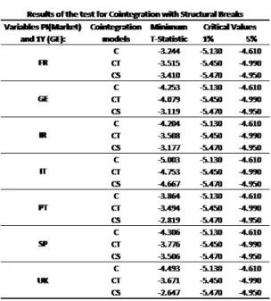
The cointegration hypothesis was tested by performing the relationship between the stock market prices and interest rates (Table 4). Bivariate cointegration was considered for this purpose, allowing for structural break tests between the price indexes of each stock market and the interest rate at 1 year of European market benchmark (GE).
This test detects regime-shift as well as stable cointegration relationships. Thus, the rejection of the null hypothesis does not entangle the instability of the cointegration relationship. The differentiation of these situations is made using stationarity tests and with the structural breaks previously presented. It is possible to infer the US influence on the European equity markets through the timing of structural breaks (Tables 1 to 3) and because both variables show prolonged upward and downward movements (resumed in Table 4).
Table 4 - Cointegration results
5. Conclusion
This paper explored possible structural changes in the stock market and interest rate variables as well as the relationship between them. With this purpose, first the ZA, the LP and the LS (1 break) were employed to test for the presence of structural breaks with unknown timing in the individual series; multiple structural breaks were then detected with BP and LM (2 breaks) tests. Secondly, the G-H test was used for cointegration between stock market prices and the interest rates for the European markets under stress and infected by the vast sovereign debt crisis since 2003. The results effectively revealed that there was a relationship between the two variables in all analyzed countries which implies important economic repercussions. Conducting monetary policy by targeting a monetary aggregate requires reliable quantitative estimates of the demand for money determined by the interest rate behavior.
It has become clear that today's equity markets around the world are no longer national markets. Stock indexes in both the US and worldwide have dropped dramatically; investors and stock traders in different markets around the world wait for new announcements given by listed companies and adjust their portfolio according to news from other markets. This phenomenon revealed how international and
interconnected the stock markets have become. While these interactions between stock markets and interest rates have been approved, more critical questions arise for both economic researchers and investors: Are these linkages only important in the short run or are there even long-run equilibrium relationships between financial markets? Equilibrium that allows investors and researchers to use information about one market to predict the performance of another in the long run? It is important for both financial, economic theory and practical asset management to know whether financial markets are cointegrated or not.
An examination of the crisis reveals that economies are already quite integrated, and this resulted in its spread from the US to the rest of the world.
References
[1] Arghyrou, Michael Georgiou, 2007. The price effects of joining the Euro: Modeling the Greek experience using non-linear price-adjustment models. Applied Economics 39(4), 493-503. [2] Bai, Jushan, Lumsdaine, Robin .L. and Stock,
James H., 1998. Testing For and Dating Common Breaks in Multivariate Time Series. Review of Economic Studies 65(3), 395-432. [3] Bai, Jushan and Perron, Pierre, 1998. Estimating
and testing linear models with multiple structural changes. Econometrica 66, 47-78.
[4] Bai, Jushan and Perron, Pierre, 2001. Multiple structural change models: A simulation analysis. Manuscript, Boston University.
[5] Bai, Jushan and Perron, Pierre, 2003a. Computation and analysis of multiple structural change models. Journal of Applied Econometrics 18, 1-22.
[6] Bai, Jushan and Perron, Pierre, 2003b. Critical values for multiple structural change tests. Econometrics Journal 6, 72-78.
[7] Baker, Malcolm, Nagel, Stefan and Wurgler, Jeffrey, 2007. The Effect of Dividends on Consumption. Brookings Papers on Economic Activity, Economic Studies Program, The Brookings Institution, 38(1), 231-292.
[8] Banerjee, Anindya, Lumsdaine, R. Robin L. and Stock, James .H., 1992. Recursive and
Sequential Tests of the Unit Root and Trend-Break Hypothesis: Theory and International Evidence. Journal of Business and Economic Statistics 10, 271-287.
[9] Ben-David, D., Lumsdaine, Robin L. and Papell, David H., 2003. Unit roots, postwar slowdowns and long-run growth: Evidence from two structural breaks. Empirical Economics 28(2), 303-319.
[10] Ben-David, D. and Papell, David H., 1995. Slowdowns and Meltdowns: Post-war Growth Evidence from 74 Countries. CEPR Discussion Papers No. 1111.
[11] Ben-David, D. and Papell, David H., 1997. International trade and structural change. Journal of International Economics 43(3-4), 513-523. [12] Chou, Win Lin, 2007. Performance of LM-type
unit root tests with trend break: A bootstrap approach. Economics Letters 94(1), 76-82. [13] Dey, Malay K. and Wang, Chaoyan, 2012.
Return spread and liquidity: Evidence from Hong Kong ADRs. Research in International Business and Finance 26(2), 164-180.
[14] Ghoshray, Atanu and Johnson, Ben, 2010. Trends in world energy prices. Energy Economics 32, 1147-1156.
[15] Gregory, Allan W. and Hansen, Bruce E., 1996. Tests for cointegration in models with regime and trend shifts. Oxford Bulletin of Economics and Statistics 58, 555-560.
[16] Kenourgios, D., Padhi, S., 2012. Emerging markets and financial crises: Regional, global or isolated shocks? J. Multinatl. Financ., 22, 24-38.
[17] Kumar, Alok. and Lee, Charles M.C., 2006. Retail Investor Sentiment and Return Comovements. The Journal of Finance LXI (5), 2451-2486.
[18] Kurov, Alexander, 2010. Investor sentiment and the stock market’s reaction to monetary policy. Journal of Banking & Finance 34, 139-149. [19] Lapavitsas, Costas, 2012. Crisis in the Eurozone.
Verso Books. [20] Lean, Hooi Hooi and Smyth, Russell., 2007a. Do
Asian stock markets follow a random walk? Evidence from LM unit root tests with one and two structural breaks. Review of Pacific Basin Financial Markets and Policies 10(1), 15-31.
[21] Lean, Hooi Hooi and Smyth, Russell, 2007b. Are Asian real exchange rates mean reverting? Evidence from univariate and panel LM unit root tests with one and two structural breaks. Applied Economics (39), 2109-20.
[22] Lee, Junsoo and Strazicich, Mark C., 2003. Minimum Lagrange multiplier unit root test with two structural breaks. The Review of Economics and Statistics 85(4), 1082-1089.
[23] Lee, Junsoo, List, John A. and Strazicich, Mark C., 2004. Minimum LM unit root test with one structural break. Appalachain State University, Department of Economics, Working Paper No. 17.
[24] Lee, Junsoo, List, John A. and Strazicich, Mark C., 2006. Non-renewable resource prices: deterministic or stochastic trends? Journal of Environmental Economics and Management 51(3), 354-370.
[25] Lumsdaine, Robin L. and Papell, David H., 1997. Multiple Trend Breaks and the Unit Root Hypothesis. Review of Economics and Statistics 79(2), 212-218.
[26] Maican, Florin G., Sweeney and Richard J., 2013. Real exchange rate adjustment in European transition countries. Journal of Banking & Finance 37, 907-926.
[27] Marashdeh, Hazem and Shrestha, Min B., 2008. Efficiency in emerging markets - evidence from the Emirates securities market. European Journal of Economics, Finance and Administrative Sciences (12), 143-150.
[28] Narayan, Kumar Paresh and Smyth, Russell, 2007. Are shocks to energy consumption permanent or temporary? Evidence from 182 countries. Energy Policy 35(1), 333-341.
[29] Nelson, Charles R. and Plosser, Charles L., 1982. Trends and Random Walks in Macroeconomics Time Series: Some Evidence and Implications, Journal of Monetary Economics 10, 139-162. [30] Nunes, Luis C., Newbold, Paul and Kuan,
Chung-Ming, 1997. Testing for unit roots with breaks: Evidence on the Great Crash and the unit root hypothesis reconsidered. Oxford Bulletin of Economics and Statistics 59(4), 435-448.
[31] Pahlavani, Mosayeb, Salman, Saleh and Sivalingam, G., 2006. Time Series Analysis of Multiple Structural Breaks in the Malaysian Economy. The Middle East Business and Economic Review (18)2, 1-13.
[32]
erron, Pierre, 1989. The Great Crash, the Oil Price Shock, and the Unit Root Hypothesis. Econometrica 57(6), 1361-1401.
[33] Perron, Pierre, 1990. Testing for a Unit Root in a Time Series with a Changing Mean. Journal of Business & Economic Statistics 8(2), 153-162. [34] Ranganathan, T. and Ananthakumar, U., 2010.
Give it a break. 30th International Symposium on Forecasting, San Diego, USA.
[35] Yu, Wei-Choun, and, Zivot, Eric, 2011. Forecasting the term structures of Treasury and corporate yields using dynamic Nelson-Siegel models. International Journal of Forecasting 27(2), 579-591.
[36] Zivot, Eric, Andrews and Donald W. K., 1992. Further Evidence on the Great Crash, Oil Price Shock and the Unit Root Hypothesis. Journal of Business and Economic Statistics 10, 251-270.